


Abstract
Standard big bang cosmology predicts a cosmic neutrino background at Tν ≃ 1.95 K. Given the current neutrino oscillation measurements, we know most neutrinos move at large, but non-relativistic, velocities. Therefore, dark matter haloes moving in the sea of primordial neutrinos form a neutrino wake behind them, which would slow them down, due to the effect of dynamical friction. In this paper, we quantify this effect for realistic haloes, in the context of the halo model of structure formation, and show that it scales as |$m_\nu ^4$|× relative velocity and monotonically grows with the halo mass. Galaxy redshift surveys can be sensitive to this effect (at >3σ confidence level, depending on survey properties, neutrino mass and hierarchy) through redshift space distortions of distinct galaxy populations.
1 INTRODUCTION
Neutrinos are an interesting component of the standard model of particles that play a number of unique roles in particle physics, astroparticle physics and cosmology. In the standard model of particle physics, they are depicted as massless and not clearly associated as Majorana or Dirac particles. Observations of flavour oscillations in solar and atmospheric neutrinos point to the existence of the neutrino mass. In cosmology, the presence of massive active neutrinos potentially resolves some of the tension between the observed galaxy counts and those predicted by the Planck cosmological parameters as suggested by Mark et al. (2014), Battye & Moss (2014) and Beutler et al. (2014).
Constraints on the mass-squared difference of neutrinos via oscillation experiments give best-fitting values of |$\Delta m_{12}^2 \equiv m_2^2 - m_1^2 = 7.54 \times 10^{-5}\,\, {\rm eV}^2$| and |$\Delta m_{13}^2 \equiv m_3^2 - (m_1^2 + m_2^2)/2 = 2.43(2) \times 10^{-3}\,\, {\rm eV}^2$| for the normal (inverted) hierarchy (Maltoni et al. 2003; Fogli et al. 2012). These constraints lead to a lower limit on the sum of the masses of these neutrinos, Mν ≡ ∑imi > 0.058 eV for the normal hierarchy and Mν > 0.11 eV for the inverted hierarchy (see Lesgourgues & Pastor 2006, 2012, for a more comprehensive review of the role of massive neutrinos in cosmology). Thus, any limit on Mν < 0.1 eV rules out the inverted neutrino hierarchy. Alternative limits on the sum of the neutrino mass Mν may also be placed by cosmological observations and measurements. Although some degeneracy exists between the Hubble constant and the neutrino mass on the background cosmology, the cosmic microwave background (CMB) temperature perturbations are affected by the neutrino mass through the early-time integrated Sachs–Wolfe effect and the lensing effect on the power spectrum. The baryon acoustic oscillations (BAO) and measurements of the CMB temperature anisotropy have placed limits on the sum of the mass of the neutrinos as Mν < 0.23 eV (Planck Collaboration XIII 2016), albeit, slightly dependent on the assumed cosmological model parameters. First described by Bond, Efstathiou & Silk (1980), galaxy surveys present yet another method to constrain the mass of neutrinos as presented in Riemer-Sørensen et al. (2012). Suppression of structure below the free-streaming scale of the neutrinos, when they first become non-relativistic, leads to a decline in the matter power spectrum (usually at the per cent level). However, in practice, galaxy power spectra are measured and so precise knowledge of the galaxy bias as a function of scale is required since the galaxies do not cluster as matter. Notwithstanding, Riemer-Sørensen et al. (2012) explored this technique in the WiggleZ Dark Energy Survey and placed an upper limit on the sum of the neutrino masses, Mν < 0.18 eV, for three degenerate neutrino species with no prior placed on the minimum sum of neutrino masses. More recent estimates by Cuesta et al. (2016) using the WiggleZ Dark Energy Survey and SDSS-DR7 LRG, together with the BAO and CMB temperature and polarization anisotropies measurements by Planck, have yielded even tighter constraints of Mν < 0.13 eV at the 95 per cent C.L. on the sum of the neutrino masses.
2 THE NEUTRINO–CDM RELATIVE VELOCITY
A complementary technique to measure the neutrino masses using their peculiar velocities relative to dark matter has been suggested by Zhu et al. (2014). The relative velocity between the neutrinos and dark matter leads to an observable dipole distortion in the cross-correlation of different tracers. This effect is similar to the relative velocity between baryons and cold dark matter, first suggested by Tseliakhovich & Hirata (2010) and explored in a number of other works, including Yoo & Seljak (2013). The neutrino particles stream coherently across the cold dark matter (CDM) haloes over a coherence/Jeans scale of 20–50 h−1 Mpc.
In this work, we provide a semi-analytic derivation of this effect in the non-linear regime, which is equivalent to the dynamical friction for CDM haloes moving in the primordial neutrino sea. The outline is as follows. Section 2 introduces the relations between velocities and density perturbations for both neutrinos and CDM in the linear regime. Section 3 examines the effect of dynamical friction on the dark matter structures due to the streaming neutrinos. We then present the methodology and expected signal to noise for detecting this effect in current and future surveys in Section 4. Finally, Section 5 summarizes our results and concludes the paper, while the appendices provide details of signal-to-noise calculations and comparison to non-linear effects in ΛCDM simulations without neutrinos.
We show the derivative of the transfer function, |$\dot{T}$|, at z = 0 for CDM and neutrinos of different masses, in Fig. 1, which demonstrates the impact of free steaming on their density perturbations. As expected, more free streaming leads to more suppression of growth on small scales for lighter neutrinos. The relative velocity power spectrum for different sum of neutrino masses (unless otherwise stated, all sum of neutrino masses assume the normal hierarchy) is shown in Fig. 2.
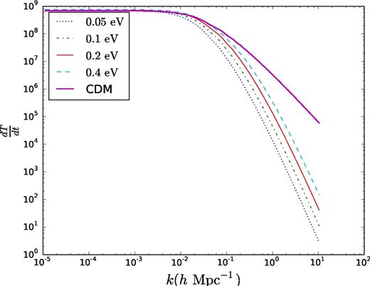
Derivative of the transfer function, |$\dot{T}(k) = {\rm d}T(k)/{\rm d}t$|, at z = 0 for CDM and neutrinos of different masses.
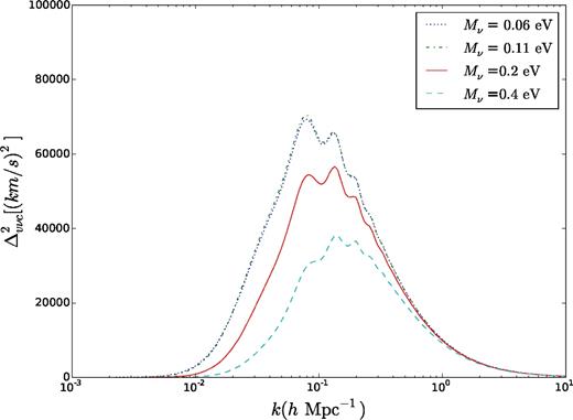
The power spectrum of the relative velocity between the neutrinos and CDM. The different curves represent different values of Mν = ∑mν (assuming normal hierarchy). The two lowest Mν’s are close due to the fact that the most massive of the three neutrinos in each sum have similar masses and dominate in the sum.
Obviously, in Fig. 2 the power lies in the range k ∼ [0.01, 1]. The rms relative velocity vνc within a sphere as a function of the radius of the window function used is shown in Fig. 3 for different sum of neutrino masses. The relative velocity between the neutrino and dark matter decreases as the mass in the neutrinos increases.
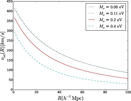
Relative CDM–neutrino velocity vνc as a function of the top-hat window function radius R for four different neutrino masses.
3 DYNAMICAL FRICTION DUE TO MASSIVE NEUTRINOS
Dark matter haloes sitting in a streaming background of neutrinos will experience a deceleration due to dynamical friction. Larger haloes experience a larger dynamical friction force than smaller mass haloes, and so larger and smaller mass haloes will have different displacements relative to the neutrino streaming direction.
In this section, we calculate the general structure of massive neutrino wakes and their dynamical friction force on dark matter haloes with a Navarro–Frenk–White (NFW) profile (Navarro et al. 1996). This drag on the halo should lead to a displacement, which is non-existent in the absence of neutrinos. This displacement Δx, in the halo's position, will be first estimated by approximating dark matter haloes as single spheres in Section 3.1. We then develop the general formalism for computing the neutrino wake in Fourier space in Section 3.2 and use it to derive dynamical friction assuming the full halo model in Section 3.3. The halo model consists of contributions from the one-halo and two-halo terms. We shall see that, while the one-halo term is equivalent to the solid sphere approximation, the two-halo term dominates the drag on small haloes.
3.1 Solid sphere approximation
3.2 Dynamical friction: general formalism
Let us briefly discuss the physical picture of a neutrino wake for a plane wave. For a finite object such as a halo (or solid sphere discussed above), a neutrino wake would form downstream, due to gravitational focusing, which is responsible for slowing down the halo (hence the term dynamical friction). The picture is qualitatively different for a CDM plane wave, as planar symmetry appears to prevent any focusing. The key here though is that, in nature, we always deal with finite wave packets, which do break exact planar symmetry. As the wave packet moves through the neutrino sea, the neutrinos with velocities nearly parallel to the wavefront (in the packet rest frame, corresponding to the singularity in equation 16) can get trapped in between the potential peaks of the travelling wave. While the neutrinos that are trapped are preferentially travelling downstream, their velocity randomizes by the time they get out, implying that they impart a net momentum on the wave packet, in the direction of the wind (see Fig. 4). Despite this qualitative difference, we shall see below that if we construct a spherical halo from the superposition of Fourier modes in equation (20), we shall recover the standard dynamical friction for an isolated sphere (equation 10).
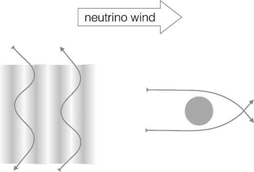
A depiction of dynamical friction experienced by a plane wave packet (left) and a compact halo (right), caused by neutrino wind (see the text for details).
3.3 Halo model
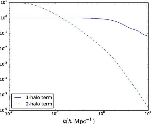
The one-halo and two-halo terms in square brackets in eq-uation (26), as a function of k, for Mhalo = 1015 h−1 M⊙ and a concentration of 4.
![The one-halo and two-halo terms of the term in square brackets including $[v^{\prime }_{\nu c}(<\!k)]^2$ as in equation (27), for Mhalo = 1015 h−1 M⊙ and a 0.2 eV neutrino.](https://oup.silverchair-cdn.com/oup/backfile/Content_public/Journal/mnras/468/2/10.1093_mnras_stx560/1/m_stx560fig6.jpeg?Expires=1750738820&Signature=rh72XH3RMEV0ivtjV3P2qSJfYOn1zC8ytbI8Z82OSwwd9X--PNjsZbeQQrXXeecoWD5LIiwyeTmLPzaSPPkGS40TgEJ8XhwmWx4OmuvdGEiJb1Cb7wWTTDp-JV2lGkkUGeKTKv-BzOe0~ulYBWa5qOJmPhY-SrhqIIti2gUu6Nn70~9J7dourA6f62bWg8Jyidem2gq996WNdlaKDbwuzj0ebtoivL0H40nGnM1Yn~ZnQN1fyzW8e0vW2vE3WFUyleqhm4ftHt5aMCaIyvy43F-DnF1mwQuOA4Af5fCH0CTg3~if4Ky1hiayQMK1-jWPNGUqgpiACyEOAF3QJpm4zQ__&Key-Pair-Id=APKAIE5G5CRDK6RD3PGA)
The one-halo and two-halo terms of the term in square brackets including |$[v^{\prime }_{\nu c}(<\!k)]^2$| as in equation (27), for Mhalo = 1015 h−1 M⊙ and a 0.2 eV neutrino.
Recall that the relative velocity between the neutrino and dark matter decreases with scale and goes to zero on very large scales (Fig. 3). On the other hand, the effects of non-linearities are expected to be more significant on smaller scales. Therefore, for concreteness, we choose a mid-point of 16 h−1 Mpc to filter relative neutrino–CDM velocity field vνc.
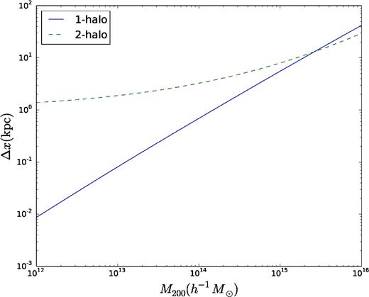
The one-halo and two-halo contribution to the displacement due to dynamical friction for a 0.1 eV neutrino. It is evident that the two-halo term dominates for all masses less than ∼1015 h−1 M⊙ where the one-halo term starts dominating.
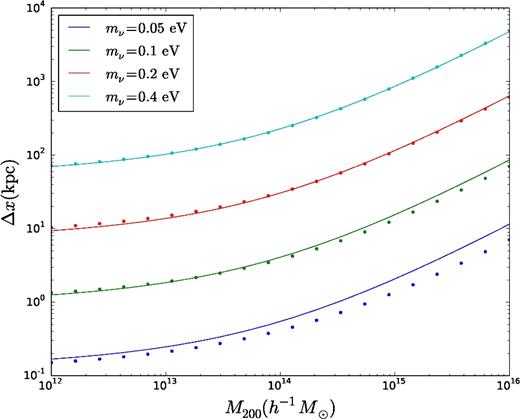
A plot comparing the fitting function in equation (31) with the calculated values for different neutrino masses. The dots are the calculated values while the line is the fitting function.
4 PREDICTED SIGNAL TO NOISE FOR NOMINAL SURVEYS
In this section, we predict the observational prospects for the detection of neutrino dynamical friction in galaxy surveys. One may be tempted to interpret equation (31) as a relative displacement/velocity of haloes of different mass due the drag by the neutrino wind. However, this is only correct given the assumption that the haloes are not in the same neighbourhood and thus have their individual wakes. To make the theoretical predictions in equation (31), we have averaged over all the haloes distributed around a given halo. In practice, this would lead to an insignificant signal in cross-correlating two haloes in the same neighbourhood. The reason for this infinitesimal signal is that they share the same large-scale neutrino wake (as depicted in Fig. 9) and thus only experience a small fraction of Δvνc. To achieve an acceptable signal-to-noise estimate, we shall focus on the effect on the large-scale distribution of haloes due to the gravity of the neutrino wake.
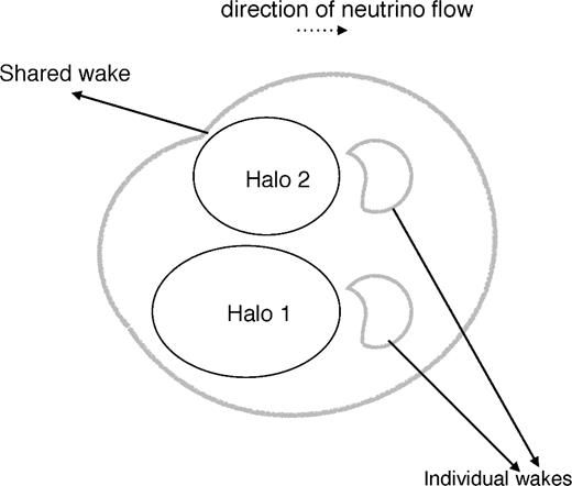
A sketch of the effect of shared wakes on the displacement of two haloes.
Thus, the density is modified by an extra time-dependent phase that manifests through the time dependence of the ν–CDM relative velocity. We aim to measure this consequence of dynamical friction due to neutrinos. To this end, we cross-correlate the densities of two tracers (possibly galaxies with different biases) in redshift space. The signal appears as an imaginary term in the redshift–space cross-correlation spectrum (see Appendix A for more details). The signal to noise for such a measurement is proportional to the difference in bias for the two populations, (bl − bf), the effective volume of the survey Veff and the time derivative of the phase term in equation (33).
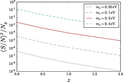
The signal-to-noise squared per galaxy as a function of redshift for various neutrino masses. This signal is estimated with a number density nl ∼ nf = 0.02 h3 Mpc− 3.
For constraints on the sum of neutrino masses, Mν, one will have to sum over the signal from the various contributing species. Fig. 11 shows these estimates as a function of the minimum neutrino mass (which can easily be related to the sum of neutrino masses, Mν) for the normal and inverted neutrino hierarchies. Even though we have assumed the number density of the luminous and faint galaxies to be ∼ 0.02 h3 Mpc− 3, Fig. 12 confirms that the signal-to-noise squared per galaxy is insensitive of the number density of galaxies. Thus, the total signal-to-noise squared is proportional to the number of galaxies Ng, Δb2 and |$m_{\nu }^6$|.
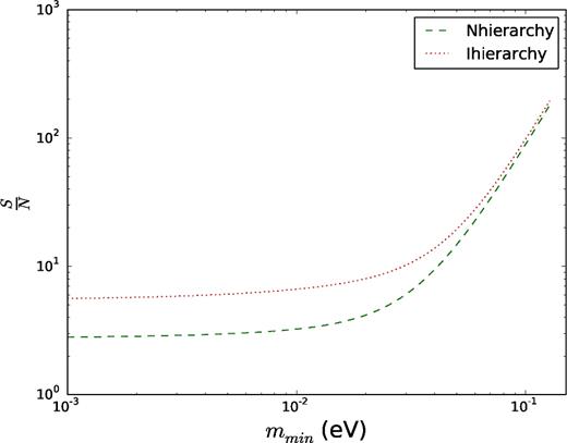
S/N for the detection of the imaginary part of the redshift–space cross-power spectrum of two tracers due to the dynamical friction effect of massive neutrinos. The dashed line and dotted line represent the S/N for the sum of the neutrino masses assuming the normal and inverted hierarchies, respectively. Both plots are for a theoretical survey assuming a volume of Veff = 1 h−3 Gpc3, Δb = 1 and nl ∼ nf = 0.02 h3 Mpc− 3.
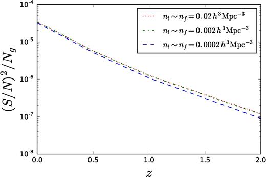
The signal-to-noise squared per galaxy as a function of redshift for various number densities, nl and nf, expected from the SPHEREX all sky survey (Doré et al. 2014). This signal is estimated for a 0.1 eV neutrino.
In Appendix B, we look at the contamination of the relative velocity signal by non-linear structure formation using ΛCDM N-body simulations, which can become comparable to kSZ measurement errors. We find that the detection of the dynamical friction effects from neutrino require about 0.1 per cent precision in the measurement of the bulk velocity. Although current experiments do not have this precision, the required precision may be met with future experiments.
5 DISCUSSION AND CONCLUSION
We have investigated the prospects for detecting a novel signal from the cross-correlation of different galaxy populations in redshift space expected in the presence of neutrinos. This is due to the dynamical friction drag experienced by dark matter haloes that move in the primordial neutrino sea. Even though the neutrinos and dark matter cannot be observed, these effects make imprints on the galaxies and should be detectable in future surveys. With current surveys, a high ( ≳10) S/N is predicted for Mν ∼ 0.2 eV, which are marginally allowed by a combination of galaxy surveys and CMB. Given the current limits on the neutrino mass, future generations of high-density redshift surveys such as DESI will be able to detect smaller mass neutrinos or sum of masses Mν < 0.1 eV.
We should note that gravitational redshift can also introduce an imaginary part to the redshift space cross-power spectrum (McDonald 2009). However, the signal from this effect is smaller than that from the effect of dynamical friction by neutrinos (for a 0.1 eV neutrino) and has a different scale dependence (∝k−1 versus the scale-dependent neutrino signal that peaks at k ∼ 0.01 Mpc h−1).
Other effects of neutrinos on large-scale structure have been discussed by Garay, Verde & Jimenez (2017). Their study serves as a method for distinguishing the mass splitting of the neutrinos given a measured constraint on the sum of neutrino masses Mν. The authors consider the effect of different neutrino masses on the power spectrum on different scales – power suppression on small scales and the change of the matter-radiation equality scale on large scales. They also claim that this method may be used to distinguish the mass splitting of neutrinos given a precise measurement of the matter power spectrum that constrains the sum of the neutrino mass. These effects become measurable on large linear scales and do not suffer from non-linearities and systematic effects. Thus, given a measured constraint on the sum of neutrino masses, this method gives another independent confirmation/test of the mass splitting seen in neutrino oscillation experiments. Yet another impact of neutrinos on large-scale structure was studied by LoVerde (2016), who proposes a method in which the neutrino mass may be constrained by the measurement of the scale-dependent bias and the linear growth parameter in upcoming large surveys. Notably, similar to our proposal, this measurement is not limited by cosmic variance.
We next discuss some of the major systematics that may affect our predictions for the signal.
5.1 Galaxy and bias
Our estimates for the S/N are based on the number density of galaxies in a survey. Using galaxies requires a good estimate of the galaxy bias. Details and precision in defining the galaxy bias (with respect to the total matter in the presence of neutrinos or to the CDM alone; Castorina et al. 2014) are required in constraining the mass of neutrinos through the suppression of power on small scales. However, we expect the exact definition of bias to be less important in extracting the dynamical friction effect, given the large-scale coherence of neutrino wind.
The extra scale dependence of the halo bias which may be due to non-linearities and the free-streaming scale of the neutrino is an extra observable proposed by LoVerde (2016). However, these affect the magnitude, not the phase, of the Fourier amplitudes at per cent level and thus should not bias our projections for neutrino drag.
5.2 Non-linearities in structure formation
The impact of non-linearities on the CDM–neutrino relative velocity was investigated by Inman et al. (2015) in a number of νΛCDM simulations. The authors were interested in the effectiveness of the simple linear theory approximation given the non-linear complexities of structure formation. Their measurements show that the relative velocity power spectra predicted from linear theory are higher than that in simulations, but are still within 30 per cent of each other for the empirically allowed neutrino masses. Reconstructing the relative velocity power spectra using the halo density field and the dark matter density field, the authors show that they are correlated with the simulations for scales k ≲ 1 h Mpc− 1 and also have the right direction of the relative velocity with a mass-dependent correlation coefficient. The magnitude of the reconstruction may be corrected for non-linearities by the ratio of the non-linear to linear CDM power spectra. This reconstruction procedure may be implemented in practice to estimate the full neutrino–CDM relative velocity power spectrum.
A more serious issue is whether non-linear effects in standard non-linear structure formation can mimic the effect of dynamical friction by neutrinos. After all, the modulation of galaxy (cross-)power spectrum, or relative velocity, by reconstructed vνc can be interpreted as a particular contribution to the galaxy bispectrum, which might be partially degenerate with the (much larger) non-linear halo bispectrum. While Appendix B provides a first look at the magnitude of this degeneracy, a more complete study of this degeneracy in νΛCDM simulations (Inman et al. 2015) is currently underway. Indeed, our preliminary analysis suggests that non linear effects are not degenerate with the expected signal from dynamical friction of neutrinos, and only have marginal impact on our predictions.
5.3 Prospects for detection
In practice, measuring the mass of neutrinos from the dynamical friction effect will be quite challenging, and requires a good knowledge and control of standard non-linear structure formation, neutrino effects and halo bias. Our S/N estimates have only included the statistical error, and control of systematic uncertainties will only come from a careful study of simulated haloes. Nevertheless, our statistical projection of S/N ≳ 3 for future surveys (see equation 35 or Fig. 10) provides an incentive for further theoretical study and improvement. The dynamical friction effect, described here, may be a powerful complement to the various ways in which neutrinos will be probed over the next decade.
Acknowledgments
We thank Derek Inman, Dustin Lang, Marilena LoVerde, Ue-Li Pen and Rafael Sorkin for valuable discussions. We also thank the anonymous referee for comments that improved the presentation of this work. This work is supported by the University of Waterloo and the Perimeter Institute for Theoretical Physics. MJH acknowledges support from NSERC. Research at the Perimeter Institute is supported by in part by the Government of Canada through Innovation, Science and Economic Development Canada and by the Province of Ontario through the Ministry of Research, Innovation and Science.
Planck collaboration XVI (2014). We use the Planck-only best-fitting values.
The advantage of using the top-hat window function is that it is localized in real space, and thus can be applied to finite real-space data. However, we do not expect our conclusions to be sensitive to this choice.
For the integral, we have assumed kmax = 1 h−1 Mpc.
REFERENCES
APPENDIX A: SIGNAL TO NOISE FROM THE GRAVITATIONAL FIELD DUE TO DYNAMICAL FRICTION
The amplitude of our signal, Im Cfl, its error Δ Im Cfl and the autopower spectrum of faint galaxies are shown in Fig. A1. This figure shows that the signal is dominated by large-scale modes. The decline of the signal at small scales suggests that the measurement is not improved by summing lots of modes. It is therefore not sample variance limited.
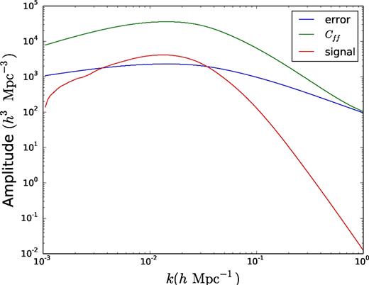
The amplitude of the signal from the imaginary part of the cross-power spectrum, the error on the signal and the autopower spectrum of faint galaxies, Cff, are shown for a 0.1 eV neutrino, nf = nl = 0.02 h3 Mpc−3 and bl = 2bf = 2.
APPENDIX B: Testing non-linear effects using N-body simulations
We shall next examine to what extent the non-linear structure formation in the standard ΛCDM model could mimic the effects of neutrino dynamical friction on cosmological haloes. We therefore use an N-body simulation without neutrinos in order to systematically account for the non-linear effects.
The signal we study is the difference in relative displacement due to neutrinos, Δx, for two different tracers, given by |$(\Delta x_1 - \Delta x_2) = \frac{1}{2} (\Delta v_{\nu c, 1}-\Delta v_{\nu c,2}) t = \frac{1}{2} v_{\rm rel} t$|, where we denote the relative velocity between tracers 1 and 2 by vrel. We want to know whether non-linear velocities due to the growth of structure on small scales could produce a signal that could interfere with the signal from massive neutrinos.
Fig. A2 a shows the measured value of α from the relative velocity of our halo samples, which is consistent with zero at <per cent level, with no evident systematic bias. A larger sample and/or simulation box will lead to lower stochastic noise in α, and can potentially reveal a systematic bias, albeit at a lower level.
![Left: fitted value of α over 100 spheres of radius r, for the (x, y, z) components (solid, dashed and dot–dashed lines) of the bulk flow of our two halo samples. Right: ΛCDM prediction for α from equation (B3) [for a 1015(h−1 M⊙ halo)] as a function of top-hat window function radius R and different sum of neutrino mass.](https://oup.silverchair-cdn.com/oup/backfile/Content_public/Journal/mnras/468/2/10.1093_mnras_stx560/1/m_stx560figa2.jpeg?Expires=1750738820&Signature=DtesjoA2BhraZRVFLXO2Zp7to53o4Jg-aSmNx5wfHjb8VntK9dSQiKJPaByi399pPFCr4wKeS2y1p6OKp3oQ~MF2nL8-jGVL24H5SQcGfpKV22HZaLVjM5pam6K3lGOZs-c9bePeq2wX9UMX6EY4MowCNBcgfVODn0TbDNZ-HMFMPRQCcXfnOI8Pe75-PPVq0r~YEDs7GOHOxxN3veZFWEn9dbNzHkVDlJ~ro~xvzg5jtbJicfbUv9T7DUxpc7gqwUQYN5~TU33~yc-wG0f08TlKCiJ8cImKKm8WK-XUg3xwD4OpV6WEaCdhps8pEW3isHnf6mt-chJksQgZfX9WPQ__&Key-Pair-Id=APKAIE5G5CRDK6RD3PGA)
Left: fitted value of α over 100 spheres of radius r, for the (x, y, z) components (solid, dashed and dot–dashed lines) of the bulk flow of our two halo samples. Right: ΛCDM prediction for α from equation (B3) [for a 1015(h−1 M⊙ halo)] as a function of top-hat window function radius R and different sum of neutrino mass.
The k integral is over the Fourier modes of the halo distribution while the k΄ integral is due to the modes from the neutrino distribution. We plot α as a function of the top-hat window function radius R and different sum of neutrino mass in Fig. A2b for a halo of mass Mh = 1015 h−1 M⊙. Clearly, the predicted value of α − 1 is quite small. For example, for Mν = 0.11 eV, the value of α − 1 is below 10−3 for all radii requiring 0.1 per cent level precision of the bulk flow to detect the neutrino effects.
