


Abstract
Stars are, generically, rotating and magnetized objects with a misalignment between their magnetic and rotation axes. Since a magnetic field induces a permanent distortion to its host, it provides effective rigidity even to a fluid star, leading to bulk stellar motion that resembles free precession. This bulk motion is, however, accompanied by induced interior velocity and magnetic field perturbations, which are oscillatory on the precession time-scale. Extending previous work, we show that these quantities are described by a set of second-order perturbation equations featuring cross-terms scaling with the product of the magnetic and centrifugal distortions to the star. For the case of a background toroidal field, we reduce these to a set of differential equations in radial functions, and find a method for their solution. The resulting magnetic field and velocity perturbations show complex multipolar structure and are strongest towards the centre of the star.
1 INTRODUCTION
Two of the most important pieces of stellar physics are their magnetic fields and rotation. They have a ubiquity across many classes of star that are otherwise governed by very different interior and exterior physics: main-sequence stars, white dwarfs, neutron stars or combinations of these in binary systems. A fundamental problem is the rich variety of ways in which rotation and magnetism interact, and the effects on stellar properties and evolution.
In this paper, we focus on one of the simplest situations within the broad class of magneto-rotational stellar phenomena: the dynamics of a rigidly rotating star with a frozen-in dynamically stable magnetic field,1 symmetric about some axis. In the case where the inclination angle χ between the magnetic and rotational axes is zero, i.e. the two axes coincide, the star is stationary. This widely studied situation has the advantage of being simple, but the disadvantage of having limited applicability to astrophysics: observations indicate that stars have a wide distribution of inclination angles (Schmidt & Norsworthy 1991; Tauris & Manchester 1998; Donati & Landstreet 2009; Rookyard, Weltevrede & Johnston 2015). A non-zero χ is essential, for example, to explain the pulsed emission seen from many neutron stars.
The dynamics of a star with non-zero χ – an ‘oblique rotator’ – is still not well understood. The classic work on the topic is by Mestel and collaborators (Mestel & Takhar 1972; Mestel et al. 1981), as discussed in Section 2. The essential idea, put forward by Spitzer (1958), is that the stellar distortion associated with the magnetic field causes it to undergo bulk motion like that of rigid-body free precession. Mestel & Takhar (1972) argue that internally this bulk motion has to be supported by time-varying and non-axisymmetric velocity and magnetic fields. Formulated in generality, this problem is intractable by analytic methods; accordingly, Mestel and collaborators made some major simplifications to produce solutions for their early studies. Various subsequent papers have adopted their ideas and solutions (see e.g. Wasserman 2003; Dall'Osso, Shore & Stella 2009; Lasky & Glampedakis 2016), but none have attempted to extend them.
The goal of the present paper is to build on the pioneering ideas of Mestel and collaborators, but to formulate them in a more rigorous and general way. The practical difference is that we are forced to perform perturbation analysis to a higher order than their work, with an accompanying increase in the complexity of the algebra. This paper is entirely concerned with the theory of this problem, and the ultimate desideratum is to obtain solutions for the perturbed velocity and magnetic fields of a fluid star with a non-zero χ. In order to keep the majority of the calculation analytically tractable, we make two key simplifications: the background magnetic field is assumed to be purely toroidal, and we employ a polytropic equation of state. For numerical reasons, we have also been forced to neglect the outermost layer of the star in our solutions. In future work, we will study the implication of our results for observed phenomena, like the distribution and time-evolution of inclination angles amongst stars, and the damping of precession.
This paper is structured as follows. In Section 2, we summarize existing models of the internal dynamics of oblique rotators, providing a critique of their applicability and suggesting how to extend them. In Section 3, we formulate the oblique-rotator problem using a perturbation scheme in two small quantities, the centrifugal and magnetic distortions, εα and εB, respectively; we show that the velocity and magnetic-field perturbations are of the same perturbative order as cross-terms involving the interaction of the stellar rotation and background magnetic field, and so finding these entails the solution of the order-εαεB perturbation equations. In Section 4, we systematically present solutions to all the lower order problems: the zeroth-order, order-εα and order-εB equations. Section 5 then addresses the problem of solving the second-order equations, through a series of stages. In Section 5.2, we reduce the full system of governing vector equations to poloidal and toroidal scalar equations. Following this, we perform a spherical-harmonic decomposition of the perturbed magnetic field (Section 5.3), yielding an infinite system of differential equations (DEs) in radial functions associated with each spherical harmonic. Superficially these appear to be ordinary differential equations (ODEs), but are, in fact, a more complicated system of differential-algebraic equations (DAEs), which cannot be solved with ODE methods. None the less, we find and present a method to solve the equations for the magnetic radial functions, when truncating at the fourth multipole (Section 5.4). In Section 6, we find closed-form expressions for the perturbed velocity field in terms of the magnetic radial functions. After this, we present results for the magnetic and velocity perturbations in Section 7. Finally, we discuss our findings and their applicability to different classes of star in Section 8, and summarize in Section 9.
2 GENERATION OF PRECESSIONAL MOTION IN A MAGNETIzED FLUID STAR
Precession is a rigid-body effect, and superficially one would not expect a fluid star (or the fluid region of a neutron star) to be able to sustain such motion. In fact, we will adopt a stellar model that is isothermal and non-convective, so we would expect only circular motion of fluid elements about the star's rotation axis. However, as argued by Spitzer (1958), a magnetic field |${\boldsymbol B}$| can provide effective rigidity to a star, since it provides a distortion (symmetric about the magnetic-field axis) away from the star's spherically symmetric hydrostatic state (Chandrasekhar & Fermi 1953). If the star is now rotated about a different axis from the magnetic one, it will undergo a secondary rotation2 about the magnetic axis, so that the bulk motion of the star resembles precession.
In this section, we begin by recapitulating the work of Mestel & Takhar (1972), who put this conceptual picture on a rigorous footing and derived the form of the secondary rotation. In doing so, we introduce notation that differs in many cases from theirs. We then describe their arguments as to why the motion is not exactly described by rigid-body free precession, and the approaches taken to finding the non-rigid internal dynamics that maintain the bulk precessional motion in both the original paper of Mestel & Takhar (1972) and a rather later follow-up study (Mestel et al. 1981). We conclude the discussion with a critique of these approaches, and describe our strategy for obtaining a more detailed solution that we believe includes the key physics missing from their work. Finally, we discuss the ordering of characteristic time-scales required for non-rigid precession to occur, and compare the various classes of magnetic star to which our analysis may apply.
We model a star as a fluid ball rotating uniformly at angular frequency α about an axis |${\boldsymbol e}_z^{(\alpha )}$|, with a frozen-in magnetic field symmetric about some axis |${\boldsymbol e}_z^{(B)}$|. The axis |${\boldsymbol e}_z^{(B)}$| is misaligned by some angle χ from the primary rotation axis |${\boldsymbol e}_z^{(\alpha )}$|. At different points in our calculation, we will need to refer to both the symmetry axis of primary rotation and that of the magnetic field, and so we form right-handed triads |$({{\boldsymbol e}_x,{\boldsymbol e}_y^{(B)},{\boldsymbol e}_z^{(B)}})$| and |$({\boldsymbol e}_x,{\boldsymbol e}_y^{(\alpha )},{\boldsymbol e}_z^{(\alpha )})$| associated with these magnetic and rotational axes, with the |${\boldsymbol e}_x$| vector being instantaneously common to both (see the left-hand side of Fig. 1). In addition, we denote the spherical polar coordinate system referred to the |${\boldsymbol e}_z^{(B)}$|-triad by (r, θ, ϕ); for the rest of this section, we shall work exclusively in this coordinate system (right-hand side of Fig. 1).
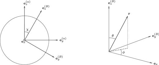
Left-hand side: the magnetic and rotational triads; we assume |${\boldsymbol e}_y^{(B)},{\boldsymbol e}_z^{(B)},{\boldsymbol e}_y^{(\alpha )}$| and |${\boldsymbol e}_z^{(\alpha )}$| are coplanar. Right-hand side: the |${\boldsymbol e}_z^{(B)}$|-triad and its spherical polar coordinate system.
2.1 The bulk motion of the star
2.2 Deviation from rigid-body precession due to internal fluid dynamics
The result at the end of the previous section suggests that the macroscopic dynamics of a rotating magnetized fluid body should resemble free precession; however, the fluid is clearly not a rigid body. This presents a question as to what degree the magnetized fluid can be regarded as rigid and hence how similar the motion of a magnetized fluid is to conventional rigid-body precession. Mestel and collaborators sought to answer this by considering the microscopic dynamics: the effect of precession on individual fluid elements and the induced non-rigid velocity field.
Since we will need to distinguish between different frames of reference here, we define for brevity the ‘α-frame’ to be the one comoving with the star's primary rotation (at frequency α) and the ‘ω-frame’ to be the co-precessing frame — i.e. the rigid-body precession frame characterized by the superimposed rotations α and ω.
An intuitive explanation for the existence of this extra velocity field, presented in Mestel & Takhar (1972), is as follows. Consider the motion of a fluid element in the α-frame; see the left-hand panel of Fig. 2. In the unmagnetized case, the element undergoes only the primary rotation α and so is stationary in the corotating frame. From Section 2.1, we anticipate that the addition of a misaligned magnetic field will cause the star to precess, and a fluid element in the α-frame will therefore undergo a slow secondary rotation (with frequency ω) about the magnetic axis. In doing so, however, the fluid element will be moved through regions of differing density. Since the background density ρ0 is spherical and the magnetic distortion δρB is symmetric about its axis, the density difference will be entirely due to the centrifugal bulge δρα. If we move to the ω-frame (Fig. 2, right-hand panel), on a macroscopic level, the entire centrifugal bulge would rotate at a rate ω about the |${\boldsymbol e}_z^{(B)}$|-axis.
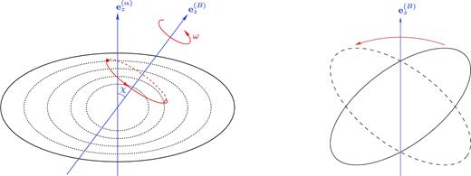
Two views of a precessing fluid star. Left-hand side: the dynamics in the α-frame, i.e. the frame rigidly rotating with rate α; right-hand side: the dynamics in the co-precessing ω-frame. We show only the centrifugal contribution to the distortion here, so that the stellar surface (the solid black line) and the isopycnic surfaces (the dashed black lines) are spheroidal about the |${\boldsymbol e}_z^{(\alpha )}$| axis. Without a magnetic field, a fluid element would be stationary in the α-frame; however, the magnetic field induces a slow precessional motion, superimposed on the normal stellar rotation. This motion will cause a fluid element (the filled red circle) in the α-frame to rotate about the magnetic axis |${\boldsymbol e}_z^{(B)}$| with period 2π/ω. A higher order velocity field |$\dot{\xi }$| is needed to prevent the fluid element from travelling through regions of varying density (crossing the density contours as shown). An alternative viewpoint of the process can be obtained from the ω-frame, in which the whole centrifugal bulge would be rotated at rate ω around the |${\boldsymbol e}_z^{(B)}$| axis were it not for the |$\dot{\xi }$| field.
At this point, we may argue for the existence of a field of non-rigid |$\xi$|-motions. In the α-frame, fluid elements undergoing rigid-body free precession (i.e. with |$\dot{\xi }= {0}$|) would be forced to sustain large-density variations over one precession period. For this reason, there will be a restoring force on each fluid element that acts to return it to its original density; hence, the precessional motion described above cannot be completely rigid. Equivalently, on a macroscopic level and in the ω frame, one would expect the global effect of the internal |$\xi$|-motions to be a restoration of the star to an instantaneous stationary equilibrium.
At this point. Mestel & Takhar (1972) used this intuitive picture to argue for the functional form of δρα, the piece of the centrifugal bulge that is time-varying in the ω-frame, by simply performing a rotation of the coordinates with respect to the rotation axis.4 They described a double-perturbation formalism in the two small parameters εα and εB – the centrifugal and magnetic distortions to the star – respectively. Crucially, they argued that one can complete the calculation merely by going to first order in each of the perturbations – i.e. using the zeroth-order, |$\mathcal {O}(\epsilon _\alpha )$| and |$\mathcal {O}(\epsilon _B)$| equations, whilst neglecting higher order cross-terms whose scaling is εαεB or higher. However, at this level, one only has a single equation to fix the three spatial components of |$\xi$|: the continuity equation, which in time-integrated form is |$\delta \rho _\alpha = -\nabla \cdot (\rho _0\xi )$|. To obtain a second condition, they specialized to motions with |$\nabla \cdot \xi = 0$|, effectively appealing to an additional buoyancy force associated with stratification; this clearly already reduces the generality of their results. Despite this, one extra relation is still required to close the system. In the first of the two papers from Mestel and collaborators (Mestel & Takhar 1972), they chose ξϕ = 0, whilst in the second one, they demanded minimization of the kinetic energy of |$\xi$| (Mestel et al. 1981).
2.3 The need for second-order perturbations
Although Mestel and collaborators claim that their results are likely to be qualitatively correct, they clearly used ad hoc assumptions to close their system of equations. This should not have been necessary, since the original problem of a rotating fluid star was perfectly well defined. In particular, it is odd that the magnetic field – by dint of which the precession was possible to start with – does not enter directly at all. Instead, in our approach, we follow the original steps of Mestel & Takhar (1972) and set up a perturbation scheme in the small parameters εα and εB, but then rigorously write out all the resulting systems of equations. By doing so, we show that the non-rigid response of the fluid to the precessional motion – encoded in the velocity field |$\dot{\xi }$| and a perturbed magnetic field |$\delta {\boldsymbol B}$| – only enters at order εαεB. The resulting hierarchy of equations – at the zeroth, first and second perturbative order – is unsurprisingly more complex than that considered in previous work, but we believe that these equations contain the minimal information required to get a reliable solution.
2.4 Key parameters for precessing magnetic stars
A number of different classes of star are thought to harbour long-lived magnetic fields and to have significant rotation rates. These are all candidates for undergoing the non-rigid precession mechanism upon which this paper is focused. To orientate the reader, Table 1 gives some typical parameters for these stars, including estimates for τA and Tω. These are made by assuming that the volume-averaged magnetic field strength is equal to the surface value Bsurf as inferred from observations. In reality, the interior field could be considerably stronger (especially if it is dominated by a toroidal component), so the absolute values we report for τA and Tω should be taken with caution – however, the ordering τA ≪ Tω will hold regardless. In addition, our estimate of Tω for a typical Ap/Bp star is in broad agreement with the results of the calculations of Mestel et al. (1981) and Nittmann & Wood (1981).
Key parameters and time-scales for different classes of potentially precessing magnetic stars.
| Class of star | Mass |$\mathcal {M}$|/g | Radius R*/cm | Bsurf/G | Tα | Estimated τA | Estimated Tω/yr |
|---|---|---|---|---|---|---|
| O star1 | 7 × 1034 | 7 × 10¹¹ | 103 | 15 d | 10 yr | 5 × 10⁷ |
| Ap/Bp star2 | 4 × 1033 | 1011 | 104 | 1 d | 0.6 yr | 3 × 10⁵ |
| Magnetic white dwarf3 | 2 × 1033 | 109 | 108 | 1 h | 0.4 h | 3000 |
| Pulsar4 | 3 × 1033 | 106 | 1012 | 0.1 s | 50 s | 2000 |
| Magnetar4 | 3 × 1033 | 106 | 1015 | 10 s | 0.05 s | 0.2 |
3 FLUID PRECESSION AS A SECOND-ORDER PERTURBATION PROBLEM
3.1 Full equations
Using the logic of the previous section, we argue that the motion of our star is close to that of a freely precessing rigid body. To some approximation, then, the motion must then consist of two superimposed rotations, one at rate α about |${\boldsymbol e}_z^{(\alpha )}$|, and the other at a much slower rate ω = αεBcos χ about the magnetic axis |${\boldsymbol e}_z^{(B)}$|, with |${\boldsymbol e}_z^{(B)}$| tracing out a cone of half-angle χ about |${\boldsymbol e}_z^{(\alpha )}$| at a rate α. However, from the point of view of an observer rotating with the body, the centrifugal bulge of size εα rotates about |${\boldsymbol e}_z^{(B)}$|, again in a cone of half-angle χ, at the slow precession frequency ω; recall Fig. 2. It is this slow density wave that produces an Eulerian density perturbation δρα(t) (see below for the precise meaning), which in turn induces the |$\xi$|-motions that encode the non-rigid response.
3.2 Perturbative scheme
In order to derive sets of perturbation equations, we first need to choose which frame to work in. There are three natural options:
The inertial frame, |$\boldsymbol \Omega = 0$|. This is conceptually simple, but in this frame, both the mass and magnetic fields are time-varying.
The α-frame, |${\boldsymbol \Omega } = \alpha {\boldsymbol e}_z^{(\alpha )}$|. In this frame, both the mass and magnetic fields are stationary to the lowest order, but individual fluid elements move in large circles about |${\boldsymbol e}_z^{(B)}$|.
The ω-frame, |${\boldsymbol \Omega } = \alpha {\boldsymbol e}_z^{(\alpha )} + \omega {\boldsymbol e}_z^{(B)}$|. In this frame, the magnetic field is stationary to the lowest order, but the |${\boldsymbol e}_z^{(\alpha )}$| axis moves about |${\boldsymbol e}_z^{(B)}$| with a period 2π/ω. Consequently, the mass field is also time-varying on the ω time-scale, inducing the |$\xi$|-motions.
We will find below that all these leading-order pieces are of sufficiently high order that they will not be needed in our analysis.
We can now insert all of these perturbative expansions into the full set of equations, to give sets of perturbation equations to be solved simultaneously. It is convenient to label these sets according to the order in εα and εB to which terms are retained in the Euler equation.
3.3 Zeroth-order equations
3.4 Order-εB equations
3.5 Order-εα equations
3.6 Order-εαεB equations
3.7 Equations of order |$\epsilon _\alpha ^2$|, |$\epsilon _B^2$| and higher
As discussed earlier, there are three different sets of second-order perturbation equations: one set with |$\mathcal {O}(\epsilon _\alpha ^2)$| terms, another with |$\mathcal {O}(\epsilon _B^2)$| terms and a third with |$\mathcal {O}(\epsilon _\alpha \epsilon _B)$| terms. We saw from the previous section that the latter set encodes the non-rigid motions in which we are interested. The reason for neglecting the other two is not that they are of a higher order – in fact, |$\mathcal {O}(\epsilon _\alpha \epsilon _B)$| quantities will never numerically be the largest of the three – but simply that they contain more mundane information.
The order-|$\epsilon _\alpha ^2$| equations merely describe a correction δραα to the result of calculating the centrifugal bulge from the order-εα equations. This correction scales with α4 and therefore does not become important except for very rapidly rotating stellar models. Analogously, the order-|$\epsilon _B^2$| equations encode a correction δρBB, scaling with B4, to the magnetic distortion as given by the order-εB calculation. Here, a stronger statement may be made: there is no known star for which the magnetic energy is anywhere near large enough to warrant including this higher order correction (Reisenegger 2009).
Although we will not consider any higher order quantities than those discussed, we note that the density perturbation δραB should be time-dependent, and therefore through a higher order analogue of the continuity equation (54) will induce a velocity perturbation of a higher order than |$\dot{\xi }$|. Similarly, δραα induces a velocity field, but merely a rapid-rotation correction to |$\dot{\xi }$|. Finally, δρBB is stationary, so the associated velocity correction is identically zero.
4 SOLUTION OF THE ZEROTH- AND FIRST-ORDER EQUATIONS
Before tackling the second-order |$\mathcal {O}(\epsilon _\alpha \epsilon _B)$| system of equations we wish to solve, we first need results from the three lower order systems of equations: the zeroth-order, |$\mathcal {O}(\epsilon _B)$| and |$\mathcal {O}(\epsilon _\alpha )$| sets. The first two are readily found in the literature, but the latter calculation is non-standard and so we report it in full.
We will specialize to the case of a γ = 2 polytropic equation of state. This has the advantage that virtually the entire calculation may be carried out analytically, and is the simplest case for which the fluid motion is compressible. Although this polytrope better mimics the pressure–density distribution of neutron stars than for other classes of star, we will argue later that many features of our solutions are likely to be applicable to a generic magnetic star. A detailed discussion of the applicability, and limitations, of our model may be found in Section 8.
4.1 The zeroth-order equations
4.2 The order-εB equations
This completes the description of order-εB quantities needed as input for the second-order perturbation equations later. In particular, although the quantities δρB, δHB or δΦB appear directly in the order-εB equations, we will not need explicit forms for these.
4.3 The order-εα equations
In the ω-frame, the centrifugal distortion δρα is neither stationary nor axisymmetric. It is sourced by the centrifugal force |$\boldsymbol \Omega _\alpha \times (\boldsymbol \Omega _\alpha \times {\boldsymbol r})$|, whose form we know from our free-precession ansatz on |$\boldsymbol \Omega _\alpha$|. Our first task is to write this force as the gradient of a scalar function.
4.3.1 The centrifugal force
4.3.2 The |$\mathcal {O}(\epsilon _\alpha )$| system as a single Helmholtz equation
4.3.3 Homogeneous solution
4.3.4 Particular solution
4.3.5 Full interior solution
4.3.6 Exterior solution and boundary conditions
4.3.7 The first-order perturbation in the density
5 SOLUTION OF THE SECOND-ORDER EQUATIONS
The above gives us a strategy to solve the second-order perturbation equations, but to proceed, we need to find explicit forms of the schematically written equations (101) and (102). To this end, we first describe a general decomposition of a solenoidal field.
5.1 Preliminaries on solenoidal fields
5.2 An explicit toroidal–poloidal split of the curled Euler equation
Our first task is to find explicit expressions for the poloidal and toroidal terms in the curled Euler equations (101) and (102), by comparing the terms with the Mie representation (106).
5.3 Equations for |$\delta {\boldsymbol B}$|
Equation (134) gives three scalar equations in four unknowns – the three components of |$\delta {\boldsymbol B}$| and the new scalar Ξ. The set of equations is then closed with the divergence-free condition on |$\delta {\boldsymbol B}$|. We are, at last, in a position to obtain a set of DEs featuring |$\delta {\boldsymbol B}$| explicitly.
For brevity, we have shown equations for general l, but by doing so, some of the above equations as written feature U and W functions with l < |m|, and in particular with negative l (e.g. the Ul − 2 terms when l = m = 1). The origin of these terms, however, is in l < |m| spherical harmonics from (157) to (159) – and these are identically zero (see the notes after these equations). Accordingly, equations (161)–(163) and those which follow them in this section are presented on the understanding that any instances of U or W functions with l < |m| are undefined and should be excluded. This is then also consistent with the original sum (136) in which the U and W functions first appeared.
5.3.1 Analysis of equations
5.4 Differential algebraic equations; conditions at the centre
Unfortunately, applying the same method to higher values of lmax does not give solutions to the original system of DAEs. We believe this is because the relations obtained at the centre from (175) become more complex – relating, for example, all quantities to a combination of |$\bar{U}_2(0)$|and|$\bar{U}_4(0)$|, instead of |$\bar{U}_2(0)$| alone. As a result, it seems that the centre conditions do not give sufficient information to fix the integration constant for higher lmax.
It would naturally have been more satisfactory to go to higher values of lmax to check the convergence of the solution in the limit l → ∞. However, the low-l, m nature of the source terms gives us reason to believe that the full l → ∞ sum will be dominated by lower multipoles, and so we anticipate that our results will be representative of the full, untruncated, solution. We will later find some hints of how the higher l components behave, in Section 7.2.
5.5 Exterior solution
To understand what boundary conditions are appropriate, let us first recall the physical meaning of the quantities in our equations. From (136) and (139), we see that the Ul functions are associated with the poloidal component of |$\delta {\boldsymbol B}$|, and the Wl functions with the toroidal component. We may, therefore, regard the two unknown quantities in the above coupled DEs as being |$\delta {\boldsymbol B}_{{\rm pol}}$| and |$\delta {\boldsymbol B}_{{\rm tor}}$|. Note that by eliminating the Ξl functions, we have produced a set of equations with no dependence on second-order fluid perturbations like δHαB; see the discussion after equation (134). This means that we only need to impose boundary conditions on the perturbed magnetic field, rather than on the fluid too.
5.6 Internal solution behaviour as outer boundary → R*
Within our model, the most natural place to impose boundary conditions matching the interior and exterior solutions would be at the stellar surface R*. A closer look at equations (164) and (165), however, indicates problems with doing so. In particular, the equations feature terms of the form |$\rho ^{\prime }_0/\rho _0$| and the radial derivative thereof, both of which diverge as r → R* for a γ = 2 polytrope.6
The divergent terms originate from the perturbed Lorentz force; see equation (51). Of these three terms, two have a denominator of ρ0 and one has a denominator of |$\rho _0^2$|; we therefore need corresponding factors in the numerators to avoid the Lorentz force diverging when ρ0 → 0. The second of the three Lorentz-force terms from (51) involves a cross-product with |${\boldsymbol B}_0$|, which, in turn, scales with ρ0, and so this term is indeed well behaved. The first and third terms will diverge, however, unless |$\nabla \times {\boldsymbol B}_0\rightarrow 0$| at least as fast as ρ0 – which it does not; it contains one term that instead scales with |$\rho ^{\prime }_0$| (this can be seen by direct evaluation of the curl of equation 58, or by applying relation (140) to |${\boldsymbol B}_0$| in the form given in equation 137), and |$\rho ^{\prime }_0$| is non-zero at R*. As originally noted by Mestel et al. (1981), this divergence is a problem before even reaching the surface, since the perturbed Lorentz force – an |$\mathcal {O}(\epsilon _\alpha \epsilon _B)$| quantity – will eventually become numerically larger than the |$\mathcal {O}(\epsilon _\alpha )$| centrifugal force from equation (27) at some radius r < R*. At this point, our perturbative ordering breaks down, and our scheme and equations become invalid.
To see how this problem would manifest itself in practice, we solved the system of equations (164) and (174) up to an outer radius Rout < R*, and investigated the behaviour of the solutions in the limit Rout → R*. As Rout was increased, the amplitude of the radial functions |$\bar{U},X$| was seen to diverge. At the inner and outer boundaries, however, the solutions were well behaved.
The simplest resolution to this problem is to place an outer boundary Rout somewhere beneath the stellar surface. For the stellar model studied in Mestel et al. (1981), this was chosen to be 0.99R*. Our numerical results from varying the cut-off radius, on the other hand, showed that the solutions were relatively insensitive to the exact cut-off value provided Rout ≲ 0.93R*; accordingly, we will place the outer boundary for the calculation at a value Rout = 0.9R*. For main-sequence stars and white dwarfs, this is an arbitrary choice, and a discussion of its validity is given at the end of this paper, in Section 8. For neutron stars, however, we can give a more quantitative argument for placing the outer boundary at 0.9R*: it is (approximately) the radius at which the star's fluid core gives way to a solid, elastic crust, and so provides a natural cut-off for our fluid calculation. Next, we discuss how our solutions might be affected by elastic forces in a neutron-star crust, if we were to extend our modelling to include this region.
5.7 Conditions in the crust of a neutron star
To extend our analysis to include the effects of a neutron-star crust, we would need to include elastic-force terms in our perturbation equations. This is not straightforward, however, as the resulting terms have a separate perturbative scaling from those in our problem. In addition, one has to define what the relaxed state of the crust is – i.e. the state in which the stresses are zero (and therefore the crust is described by fluid terms alone). In a real neutron star, the crust's elastic stress pattern is likely to be complicated and to depend on the star's rotational and seismic history.
For the purposes of this paper, we just wish to make a qualitative assessment of how elasticity might modify our solution; for this, there are two limiting cases. In one limit, the crust is so strong that it can maintain its spheroidal centrifugal distortion even as the star's instantaneous rotation vector is substantially misaligned from the primary rotation vector (recall Fig. 2); the crust would therefore undergo rigid-body free precession with no additional |$\xi$|-motions. In the other limit, the crust is so weak that elastic forces have negligible contribution at all perturbative orders we consider. We will argue next that a neutron-star crust falls between these two limits. A separate issue to consider is whether the stresses could be large enough to exceed the elastic yield limit of the crust. Finally, we discuss the coupling between the crust and core in a magnetized precessing neutron star.
5.7.1 Importance of elastic force terms
The conclusion we draw from this is that the crust is weak enough that the centrifugal bulge will always remain approximately symmetrical about the primary-rotation axis, but strong enough that our solutions for |$\dot{\xi }$| and |$\delta {\boldsymbol B}$| could be radically altered in the crustal region. Since we are obliged to place an outer boundary some distance within the star anyway, to ensure the validity of our perturbative scheme, we find it natural simply to exclude the crust from our modelling altogether, and place an outer boundary at the crust–core interface, r = 0.9R*.
5.7.2 Exceeding the crustal breaking strain
5.7.3 Crust–core coupling
This paper focusses on fluid stars whose only ‘rigidity’ comes from their magnetic fields. By contrast, the solid crust of a neutron star can, of course, undergo conventional rigid-body free precession without the aid of any magnetic field – provided it has some permanent distortion misaligned from the rotation axis. If we temporarily ignore the magnetic rigidity of the core, this fluid region will be unable to precess, and the resulting dynamics of the neutron star will be a precessing crust atop a rigidly rotating core.
In fact, the star's magnetic field would generally thread the crust and core, and couple together the two regions on an Alfvén time-scale τA. In the case where |$\tau _{\rm A} \lesssim \sqrt{T_\alpha T_\omega }$|, Levin & D'Angelo (2004) showed that the core's motion is strongly coupled to that of the crust, so that the whole star would precess as one.8 Thus, in general, a neutron star's precession should combine two effects: the non-rigid precession on which this paper is focused (related to the magnetic distortion of the fluid) and a coupling to the rigid-body precession of the crust (related only to the crust's permanent distortion). We close by noting that for our particular stellar model, the latter effect may not actually occur: purely toroidal magnetic field lines are always non-radial and so no field line will cross from the crust to the core.
5.8 Boundary conditions for our model
Our system of equations, (164) and (174), is second-order in |$\bar{U}_l$| and first-order in Xl. This means that for each |$\bar{U}_l$|, we need to impose two boundary conditions, and for each Xl, we need to impose one boundary condition.
The boundary conditions used in our solution of the ODE system, (164) and (174), are summarized in Table 2.
Summary of boundary conditions for our problem, truncated at l = lmax = 4. There is one fewer boundary condition for m = 2, since X1 does not exist for this case.
| m | Centre | Crust–core boundary |
|---|---|---|
| |$U^{\prime }_2(0) = 0$| | |$R_{\rm out}U^{\prime }_2(R_{\rm out})+4U_2(R_{\rm out}) = 0$| | |
| 1 | |$U_4(0) = -\frac{55}{6\sqrt{6}}U_2(0)$| | |$R_{\rm out}U^{\prime }_4(R_{\rm out})+6U_4(R_{\rm out}) = 0$| |
| |$X_3(0) = -\frac{7}{12}\sqrt{\frac{35}{2}}U_2(0)$| | X1(Rout) = 0 | |
| |$U^{\prime }_2(0) = 0$| | |$R_{\rm out}U^{\prime }_2(R_{\rm out})+4U_2(R_{\rm out}) = 0$| | |
| 2 | |$U^{\prime }_4(0) = 0$| | |$R_{\rm out}U^{\prime }_4(R_{\rm out})+6U_4(R_{\rm out}) = 0$| |
| |$X_3(0) = -\frac{2}{15\sqrt{7}}U_2(0)+\frac{207}{550}\sqrt{\frac{3}{7}}U_4(0)$| | – |
6 THE |$\xi$|-MOTIONS
We have derived a set of DEs whose solution gives us |$\delta {\boldsymbol B}$|. Together with the simple solution for δρα (see equation 95), this gives us enough information to solve for the perturbed velocity field |$\dot{\xi }$|, using the perturbed continuity and induction equations (104) and (105). In this section, we show that |$\dot{\xi }$| may be found explicitly in terms of the magnetic functions |$U_l^m$| and |$W_l^m$|, through relatively simple algebraic manipulation of equations (104) and (105).
We first need, therefore, to rewrite the general expression for |$\delta {\boldsymbol B}$| from (136) in its Mie representation. Note that we could, in fact, commence with |$\delta {\boldsymbol B}$| in the simpler form given in (172), which is specific to our problem. We prefer, however, to consider the general case, so that parts of the analysis here may be directly applied to other problems (for example, precession of a magnetic star where |${\boldsymbol B}_0$| is a poloidal or mixed poloidal-toroidal field).
7 RESULTS
Finally, we come to the results of solving equations (164) and (174), with the boundary conditions given in Table 2. Having recast the original system of DAEs into a simpler system of ODEs, the numerical solution then becomes fairly straightforward, subject to a few numerical subtleties that we detail in Appendix B. In what follows, the radial functions are of course time-independent, but the results for |$\delta {\boldsymbol B}$| and |$\dot{\xi }$| are presented for t = 0. Over a period of 2π/ω, these three-dimensional figures would rotate around the z-axis.
7.1 The poloidal and toroidal radial functions
We recall that the fundamental quantities to solve for were the toroidal radial functions |$X_l^m\equiv W_l^m/r$| and the poloidal radial functions |$\bar{U}_l^m\equiv iU_l^m$|. From these, one can find the perturbed magnetic field |$\delta {\boldsymbol B}$|, by using equation (172), and the perturbed velocity field – the |$\xi$|-motions – by using equations (219)–(221). We begin by plotting these poloidal and toroidal radial functions, in Fig. 3. All of these functions appear to tend to zero at the origin, suggesting that the central boundary conditions described in Section 5.4 were actually unnecessary and that simply imposing the vanishing of all variables would have been sufficient. Having tried this, however, we found that the resulting functions were not solutions of the original system of DAEs, (164) and (165). Numerically, the U and X functions have tiny – but non-zero – values at the centre, and fixing the correct ratios between them (those of Table 2) is, in fact, crucial for getting a solution to the DAEs.
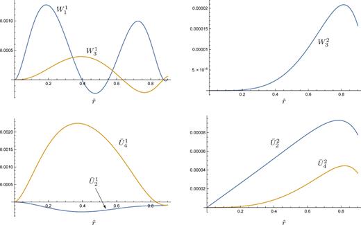
Plots of the radial functions of |$\delta {\boldsymbol B}$| against dimensionless radius |$\hat{r}$|, for lmax = 4, inclination angle χ = π/4, dimensionless primary rotation frequency |$\hat{\alpha }= 0.1$| and dimensionless background magnetic field strength |$\hat{\Lambda }= 0.1$| (see equations 229–231 for formulae to redimensionalize these to physical stellar parameters). Varying χ only changes the amplitude of the results, and the relative size of the m = 1 and 2 components; in the limit of an orthogonal rotator, only the m = 2 functions are non-zero.
The m = 1 functions in Fig. 3 are numerically larger than their m = 2 counterparts for the chosen inclination angle of χ = π/4; only very close to the orthogonal-rotator case (χ = π/2) do the m = 2 perturbations become larger than those for m = 1. Perhaps the other most significant feature to note is that the |$\bar{U}_2^1$| function is a factor of 8 smaller than the |$\bar{U}_4^1$|, i.e. the quadrupolar perturbed magnetic field is significantly smaller than the l = 4 component. This contradicts one's experience from simpler calculations – in axisymmetric magnetic equilibria, for example, the solutions feature odd l and are dominantly dipolar, with the power in the multipoles falling off monotonically (Ciolfi et al. 2009; Lander, Andersson & Glampedakis 2012).
The solutions plotted in Fig. 3 are numerical, with no closed-form expressions, and so are of limited applicability. For this reason, we next explore the scaling of the solutions with rotation rate, field strength and inclination angle, and present polynomial approximations to the radial functions |$\bar{U}_l^m$| and |$W_l^m$|.
From equations (164) and (165), the source terms for the radial functions |$U^m_l,X^m_l$| are of the form |$\tilde{\Psi }_l^m/\Lambda$| and |$\tilde{\Upsilon }_l^m/\Lambda$|; comparing with equations (A4) and (A5), we see that the m = 1 source terms are proportional to α2Λsin (2χ) and that the m = 2 source terms are proportional to α2Λsin 2χ. We therefore expect the same scaling for the radial functions |$U^m_l,X^m_l$|, which we have confirmed by solving the equations for different values of α, Λ and χ (plots omitted for brevity).
Note that the number of terms required for an accurate approximation of each function differ, and that the minimum and maximum powers featured in the above set of relations are r and r8, respectively. Constant (i.e. r0) terms are unnecessary, since the U and X functions are very small at the origin, and the W functions are exactly zero (since |$W_l^m = rX_l^m$|, and the |$X_l^m$| functions are finite at r = 0); see Fig. 3.
7.2 Behaviour of higher multipoles at the centre
As discussed in Section 5.4, we are limited to truncating our solutions at a maximum angular index l = lmax = 4, and we anticipate that higher multipoles will gradually become negligible. However, we have already seen from Fig. 3 that the magnitude of the multipolar functions does not decrease monotonically, and so we would like some idea of the relative strength of higher multipoles.
Returning to our system of DAEs, (164) and (165), we note a few features. They couple together X functions over an l-range of 4, from Xl − 2 to Xl + 2, and |$\bar{U}$| functions over an l-range of 6, so it is natural to expect solutions to have significant contributions from many multipoles. The highest multipoles in the source terms, on the other hand, are an l = 4 piece of |$\tilde{\Psi }$| and an l = 3 piece of |$\tilde{\Upsilon }$| (see Section A). From the way the source terms enter the DAEs, this means that the l = 5 system of equations is the last to contain any explicit source, through the |$\tilde{\Upsilon }_{l-2}$| term of equation (165). For all higher values of l, the DAEs merely relate different |$\bar{U}$| and X functions to one another, and the higher l functions are only non-zero by virtue of coupling to their lower l counterparts.
In lieu of solving the full system of DAEs for high lmax, we may evaluate the equations at the centre of the star – as done for the second DAE, (165), in Section 5.4. For r = 0, all source terms vanish (as in the full DAEs at high l), and we simply have a system of algebraic simultaneous equations relating the values of different functions at the centre, |$\bar{U}_l(0)$| and Xl(0). When truncating for odd values of lmax, the equations may be ‘solved’ to give each quantity as a fraction of X1(0), thus giving some idea of the way different multipoles couple together, and their behaviour at high l. For lower values of lmax, the results show some variation with the exact truncation value, so we terminate at lmax = 101, well after the point at which any variation can be seen.
We plot the results of this experiment in Fig. 4, where we see that the quantities Xl(0)/X1(0) and |$\bar{U}_l(0)/X_1(0)$| decay in an oscillatory manner with increasing l, alternating between negative and positive values, rather than in a more predictable monotonic manner. We also see that the Ul(0) quantities decay far more slowly, with even the l = 24 multipole being more than 1 per cent of the value of X1(0); by contrast, every Xl(0) quantity with l > 3 is below 1 per cent of X1(0).
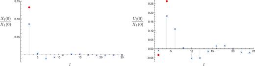
Setting the radius to zero in the original system of DAEs, (164) and (165), results in a system of simultaneous algebraic equations. We truncate these at lmax = 101 to solve them, plotting the results for l ≤ 25 here. As solutions, we find the relative magnitudes of different multipoles |$\bar{U}_l(0),X_l(0)$| at the centre, as a fraction of the value of the dipole piece X1(0) there (blue crosses). This suggests that the U functions fall off more slowly with increasing l than the X functions. For reference, the maximum values of U2, U4 and X3 from our full solution are plotted as ratios of the maximum value of X1 (filled red circles).
The only rigorous statement that one can make about Fig. 4 is, of course, that it shows the solutions to the DAEs with r set to zero. Nonetheless, we believe that it also captures the essence of how higher multipoles couple together in our problem. Evidence in favour of this is the fact that it predicts the magnitudes of |$\bar{U}_2^{\rm max}/X_1^{\rm max}$|, |$\bar{U}_4^{\rm max}/X_1^{\rm max}$| and |$X_3^{\rm max}/X_1^{\rm max}$|, from our lmax = 4 solutions, in the correct order, and in particular the fact that |$\bar{U}^1_2$| is far smaller than |$\bar{U}_4^1$| and has the opposite sign.
7.3 Magnetic-field perturbations
Having found solutions for Ul and Wl, we may now insert these into equation (172) to find |$\delta {\boldsymbol B}$|. The resulting field configuration is complicated, and we have found it clearest to separate it into its poloidal and toroidal components. First, in Fig. 5, we plot the magnitudes of these components. Broadly speaking, the perturbed magnetic field is strongest towards the centre, and the toroidal component is about double the strength of the poloidal one. For most values of the inclination angle, the m = 1 component dominates over m = 2, so the near-aligned (χ = π/16) and near-orthogonal (χ = 7π/16) results are visibly similar. For χ = π/2, when the magnetic and rotation axes are orthogonal, there is only an m = 2 component. However, this situation is actually stationary (and therefore does not correspond to precession); from equation (7), we see that ω = 0 for χ = π/2, and consequently (by equation 201), |$\mathrm{\partial} (Y_l^m(\theta ,\lambda ))/\mathrm{\partial} t = 0$|.
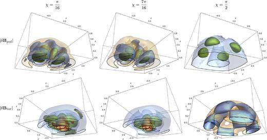
Three-dimensional contour plots showing the magnitude of the perturbed magnetic field, separated into its poloidal (top row) and toroidal (bottom row) components. Note that viewing angles differ by π/2 for the poloidal and toroidal plots. The results are symmetric about the z = 0 plane, so we show only the Northern hemisphere. Results are shown for three different values of inclination angle χ. Contours are colour coded so that the blue contour represents a field strength double that of the light brown contour, green is double the value of blue, and red is double the value of green. For a fixed inclination angle, the contour colouring is fixed, so that poloidal and toroidal components may be compared directly, but different inclination angles use different keys. The m = 1 field vanishes for the case of an orthogonal rotator (χ = π/2), leaving only the m = 2 component, and resulting in a very different-looking field (which is actually time-independent). However, the m = 2 component is generally weak, so that even the near-orthogonal configuration (χ = 7π/16) is similar to the near-aligned model (χ = π/16).
Next, we show the direction of the magnetic field, in Fig. 6. The clearest visualization we could find was to plot the poloidal and toroidal unit vectors over a nested sequence of constant-radius shells with r/R* = 0.2, 0.4, 0.6 and 0.8. Comparing the field across consecutive shells should, hopefully, allow the reader to visualize the full three-dimensional field-line structure. The toroidal component is clearer, since (by definition) its field lines run along constant-r shells. For the poloidal component, note that the blue and white patches are in roughly the same position on each contour, meaning that a given field line moves towards the centre of the star through the blue regions, then bends back and comes out through a neighbouring white region to its ‘starting’ location, thus forming a closed loop (as dictated by the requirement that |$\nabla \cdot \delta {\boldsymbol B}= 0$|).
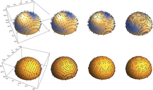
The direction of the perturbed magnetic field, plotted along a series of hemispherical shells beginning near the centre and ending near the surface. From left to right, the shells represent r/R* = 0.2, 0.4, 0.6 and 0.8, respectively. The upper row of plots shows the unit poloidal vector and the lower row the unit toroidal vector. Since arrows into and out of contours are hard to distinguish, we use colour coding for the strength of the radial field component: blue represents a region of field lines pointing towards the centre of the star, whilst white indicates outwards-pointing field lines. This only applies to the poloidal-field plots, as toroidal fields are, by definition, non-radial, and so their arrows are all tangential to the hemispherical shells. Each poloidal/toroidal plot is viewed from the same (x, y) position as in Fig. 5, but from above – i.e. for a z > 0 position, unlike the z < 0 vantage points of Fig. 5. To save space, the axes and bounding box are only drawn for the left-hand plots. Finally, we take χ = π/16 for all plots, though there is little variation of the field's direction with inclination angle.
7.4 |$\xi$|-motions
At last we come to the |$\xi$|-motions: the non-rigid velocity field present in a precessing fluid star, and the original goal of this paper. We recall that these may now be calculated from our solutions |$\bar{U}_l,X_l$| using equations (219)–(221). As for |$\delta {\boldsymbol B}$|, we separate the information about |$\dot{\xi }$| into two figures, one showing the magnitude of |$\dot{\xi }$| and the other its direction. The contours of |$\dot{\xi }$|, shown in Fig. 7, represent smaller differences than those used above for |$\delta {\boldsymbol B}$| – the speed |$|\dot{\xi }|$| only differs by a factor of |$\sqrt{2}$| between neighbouring contours, and therefore only varies by a factor of 2 across most of the stellar interior. Like the perturbed toroidal field from the lower panels in Fig. 5, the speed is greatest in a torus centred on the origin and aligned along the x = 0 plane. For the near-aligned case (χ = π/16), |$\dot{\xi }$| is approximately reflection symmetric about the x = 0 plane, but as the inclination angle is increased, the speed lowers more quickly in the x < 0 region (χ = 7π/16 plot). Finally, as mentioned in the previous section, |$\dot{\xi }= {0}$| for the limiting case of χ = π/2.
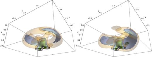
Three-dimensional contour plots showing the magnitude of |$\dot{\xi }$|, for χ = π/16 (left-hand plot) and χ = 7π/16 (right-hand plot). The details are the same as for Fig. 5, except that each contour represents a value |$\sqrt{2}$| times that of the last, meaning that the innermost contour has twice the value of the outermost.
The direction of |$\dot{\xi }$| is shown in Fig. 8. Close to the centre and to the outer boundary, the velocity is roughly tangential to constant-r shells, but in between, it has a large radial component. As for the poloidal-field direction plots, the blue and white patches are in the same location for each of the four shells in Fig. 8, meaning that there is a meridional circulation of fluid, with streamlines moving towards the centre of the star through the blue regions and back out through the white regions. Unlike the magnetic-field case, however, these streamlines do not need to close, since |$\nabla \cdot \dot{\xi }\ne 0$| (i.e. the flow is compressible). Not restricting to incompressible flow was, in fact, the place at which our approach first diverged from that of Mestel & Takhar (1972); recall the discussion of Section 2. For this reason, it is logical to close this section by looking at the behaviour of |$\nabla \cdot \dot{\xi }$| itself.
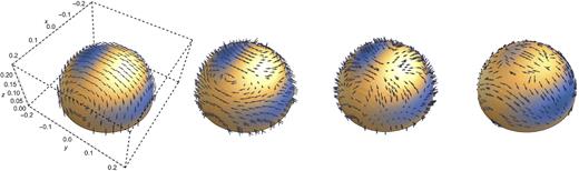
The direction of the |$\dot{\xi }$| vector field on constant-radius shells of r/R* = 0.2, 0.4, 0.6 and 0.8 (left to right), for χ = π/16. See the caption of Fig. 6 for details.
In Fig. 9, we plot the divergence of |$\nabla \cdot \dot{\xi }$|, normalized by |$|\dot{\xi }|/r$| to give a dimensionless quantity. In a barotropic star, one cannot assume incompressible motions, and indeed we see that |$\nabla \cdot \dot{\xi }$| deviates greatly from zero, especially in the outer regions. Thermal- or composition-gradient stratification in real stars would provide some additional buoyancy force to suppress compressible motions, but for a given model, one still needs to account for such a buoyancy force consistently, and to verify it is sufficiently strong to impose |$\nabla \cdot \dot{\xi }= 0$|. Fig. 9 gives an idea of how and where such forces would have to act to ensure |$\nabla \cdot \dot{\xi }= 0$|.
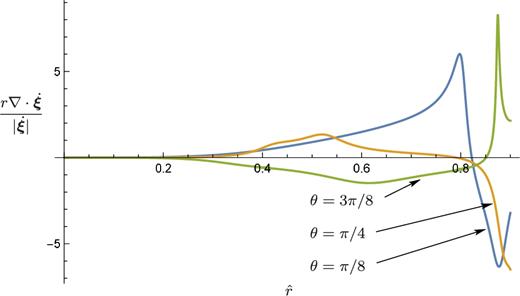
Divergence of |$\dot{\xi }$|, normalized by the speed |$|\dot{\xi }|$| divided by the radius, to make a dimensionless quantity. We show the behaviour of this quantity for λ = π/2 and three values of θ, as labelled. This plot demonstrates that for barotropic stellar models, the higher order motions in a precessing fluid star are, in fact, highly compressible. It also gives an idea of how strong buoyancy forces would need to be in order to produce the incompressible motions discussed in Mestel & Takhar (1972).
8 DISCUSSION
This paper has been concerned with a detailed description of the dynamics of a rotating magnetized star, in the general ‘oblique rotator’ case when the magnetic and rotational axes are misaligned by some angle 0 < χ < π/2. The star's bulk motion is that of free precession, but sustaining this in a fluid star requires additional dynamics in the interior: time-dependent velocity and magnetic fields. The concept of non-rigid precession was first described by Mestel & Takhar (1972), who produced simplified models of the perturbed field |$\dot{\xi }$| using first-order perturbation equations. A new calculation of |$\dot{\xi }$| was presented in Mestel et al. (1981), who also used this, in turn, to calculate magnetic field perturbations, given a poloidal background field. Nittmann & Wood (1981) performed the same analysis for a toroidal background field.
In this paper, we argue that a consistent solution for both |$\dot{\xi }$| and |$\delta {\boldsymbol B}$| can only come from solving a higher order set of equations than those previously considered. A large part of the work presented here involves a detailed formalism to describe these perturbations (Section 3), algebraic manipulation to reduce them to a set of DEs in radial functions (Section 5) and then solving these (Section 7 and Appendix B).
In order to make the problem tractable, we have had to make a number of assumptions, and now need to consider how these affect the validity of our model when applied to different classes of star. None the less, we emphasize that our model contains the minimum essential physics for non-rigid precession, and so everything that follows concerns additional effects. Even when our assumptions are unjustifiable, then, the work presented here can be regarded as a ‘background’ model upon which to build.
The most major simplification we have made is assuming a toroidal background magnetic field. Purely toroidal fields, like purely poloidal fields, suffer rapidly growing dynamical instabilities – and so cannot be realistic models of stellar magnetic fields (Tayler 1973), which must instead feature both poloidal and toroidal components. However, in the absence of an additional stabilizing mechanism, there are indications that even mixed poloidal–toroidal fields are generically unstable (Lander & Jones 2012; Mitchell et al. 2015). On the other hand, toroidal-dominated stable equilibria have been found for stellar models with an additional thermal-buoyancy force (Braithwaite 2009). The issue of stable magnetic equilibria is not fully settled, but if the toroidal component is generically the dominant one in stars, our results may indeed be a reasonable first approximation to their precessional dynamics.
For a stellar model with a purely poloidal field, we believe that an analogous analysis to ours could be carried out. However, whilst a toroidal field has a component only in the direction of one spherical–polar coordinate (the azimuthal one, λ), a poloidal field's depends on the other two (r and θ), suggesting that spherical–polar coordinates will not be appropriate for studying this problem. Instead, one can work in a coordinate system fitted to poloidal-field lines (Bernstein et al. 1958), in which case all the steps of our toroidal-field calculation should be tractable for a poloidal field too. There is, however, no coordinate system in which a mixed poloidal–toroidal field becomes similarly simple (see e.g. Tayler 1980); for a stellar model with such a background field, it seems inevitable that a fully numerical approach would be required.
Neutron stars: Most of the assumptions made in this paper are typical ones in the context of neutron-star modelling. This is certainly not equivalent to saying that they are all justifiable on physical grounds, however, so each needs further attention. The γ = 2 polytrope we adopt is quite suitable for a single-fluid model of a neutron star, but the cores of mature neutron stars are better described by a two-fluid equation of state in which the neutrons are superfluid; simple magnetic equilibrium models for mature neutron-star cores may be found in which each fluid component obeys its own polytropic relation (Glampedakis, Andersson & Lander 2012; Lander et al. 2012). The neutron superfluid will decouple from the precessional dynamics we consider in this paper, and so only the charged component is relevant. This component is, however, better described by a polytropic index γ ≈ 3/2.
It is reasonable to assume that no additional buoyancy forces enter the precessional dynamics of a mature neutron star. A neutron star in equilibrium has a density-dependent fraction of neutrons to protons. When the neutrons are not superfluid, displacing a fluid element results in chemical reactions that convert between neutrons and protons to restore the equilibrium fraction of protons and neutrons, and this represents a buoyancy force associated with the composition-gradient stratification (Reisenegger & Goldreich 1992). However, these reactions are strongly suppressed (along with the associated buoyancy) when the neutrons are superfluid. In addition, neutron stars become isothermal very early on in their life, so there is negligible thermal-gradient stratification. Finally, we have already argued (in Section 5.7) that crustal elasticity and the matching between crust and core could seriously modify our solutions in the outermost region, 0.9R* ≤ r ≤ R*, and so we considered it wisest to exclude this region altogether, and place the outer boundary for our solutions at a radius of 0.9R*.
The most significant neutron-star physics we have failed to account for is the superconducting nature of the stellar core. Since most of this region is believed to form a type-II superconductor, however, the magnetic field will still penetrate the core and produce a macroscopically uniform magnetic force (Baym, Pethick & Pines 1969). The conceptual picture should thus remain intact: the magnetic field lends rigidity to the fluid, inducing bulk precession but at the expense of requiring additional internal motions and magnetic-field perturbations. Quantitatively, however, the nature of these perturbations will undoubtedly be different – and qualitatively we would expect them to scale with the superconducting magnetic force9 ∝Hc1B ∼ 1015B instead of the normal Lorentz force ∝B2 (Easson & Pethick 1977; Wasserman 2003).
The velocity field |$\dot{\xi }$| represents a ‘macroscopic’ coupling between the star's rotation and magnetic field. In a neutron-star core with type-II superconducting protons and superfluid neutrons, however, there is a competing ‘microscopic’ coupling mechanism: the interaction of rotational neutron vortices with magnetic proton fluxtubes (Ruderman, Zhu & Chen 1998; Link 2003). Ascertaining the relative importance of these two mechanisms would be an important step towards a quantitative picture of non-rigid neutron-star precession.
White dwarfs: Unlike neutron stars, white dwarfs form a broad class of stars, with differences in chemical composition and the physics governing their different regions. The major sub-division of white dwarfs of relevance to this paper is between the magnetic and non-magnetic white dwarfs. Like neutron stars, magnetic white dwarfs have field strengths spanning several orders of magnitude, but with an upper limit of ≲109 G. Many of these strongly magnetized objects have, like magnetars, long rotation periods, although there are some rapidly rotating and highly magnetized white dwarfs (Ferrario et al. 2015) – the ideal combination for relatively short precession periods.
The equation of state for a white dwarf is a degenerate Fermi gas. In the high-density limit, this reduces to a γ = 4/3 polytrope, and in the low-density limit to a γ = 5/3 polytrope (Nauenberg 1972). For lower densities, then, the γ = 2 relation adopted here is probably not an egregious approximation to white dwarf matter. Imposing an outer boundary below the surface is also justifiable, since the degenerate core of white dwarfs gives way abruptly to a low-mass non-degenerate envelope region – although the envelope is only ∼30 km (Althaus et al. 2010), meaning that a more appropriate radius to impose the outer boundary at would be ∼0.997R* (taking care that the perturbative scheme is still applicable at this radius; see Section 5.6).
In this work, we have assumed a fluid region that extends to the stellar centre, which is not always the case for white dwarfs: As they become older and colder, white dwarfs begin to form solid cores (Van Horn 1968), with the crystallization proceeding from the centre outwards and solidifying the whole star over a time-scale of ∼109 yr (Iben & Tutukov 1984). Elasticity will then affect the induced velocity and magnetic-field perturbations in the solid core; for a sufficiently rigid core lattice, these perturbations would become negligible, and the core's motion would then be well described by standard rigid-body free precession. Finally, more detailed modelling of white dwarf precession should account for the fact that these stars are non-barotropic, with stratification due to both composition and thermal gradients.
Non-degenerate (main-sequence) stars: With some caveats, our analysis applies to objects along the upper part of the main sequence of non-degenerate stars. Upper main-sequence stars have higher masses and more simple field topologies than other non-degenerate stars, and since their envelopes appear to be in radiative equilibrium (rather than convective), dynamo action seems unlikely. The conclusion is that the magnetic fields in these envelopes are likely to be in dynamically stable equilibrium states. Of these stars, the most highly magnetized are the chemically peculiar A- and B-type stars, with field strengths up to ∼104 G. Upper main-sequence stars with strong magnetic fields tend to rotate far more slowly than their weakly magnetized counterparts, such as the normal A and B stars (Donati & Landstreet 2009).
In the radiative envelopes of main-sequence stars, our analysis is broadly applicable, but as for white dwarfs, it should be modified by the inclusion of a thermal buoyancy force. This will constrain the form of |$\dot{\xi }$| and |$\delta {\boldsymbol B}$|, but in a way that can only be confirmed by including thermal effects in a self-consistent matter in the whole analysis. As for partially crystallized white dwarfs, our analysis will not be valid all the way to the centre of main-sequence stars. In this case, the reason is the presence of an inner core region where vigorous convection disrupts and regenerates the magnetic field – and so our assumption of a large-scale stable background magnetic field becomes invalid here. Moving to the outer boundary, there is no distinct outer region of the radiative zone where one would expect the |$\xi$|-motions to stop. Our approach requires us to cut off the solution before reaching the stellar surface R* (see Section 5.6), but as long as we choose an outer boundary close to R*, we will only be neglecting a small, low-density region of the star.
For all classes of star, the internal velocity and magnetic fields solved for in this paper may have significant effects on their evolution and dynamics. In particular, since they couple the star's rotation and magnetic fields, the dissipation of these motions could cause the evolution of the inclination angle (Spitzer 1958). For toroidal fields - the case considered here - the dissipation will tend to cause the star to become an orthogonal rotator, χ → π/2; for poloidal fields, χ → 0 (Mestel & Takhar 1972). For the more realistic case of mixed poloidal–toroidal fields the evolution of χ will be dictated by the dominant field component,10 and so observations of this evolution could allow one to infer details of the star's internal magnetic field. Although we do not intend to tackle a fully self-consistent evolution of dissipative processes, a qualitative discussion of this and applications to astrophysics will be presented in a follow-up paper.
9 SUMMARY
We have presented a formalism and solution method for models of rotating magnetic stars with misaligned rotation and magnetic axes – sometimes known as oblique rotators. We began with arguably the simplest necessary pieces of physics to describe this problem: a rigid primary rotation of the star, and a large-scale m = 0 dipolar toroidal magnetic field. Despite this simplicity, we have found that the dynamics of such stars involve internal velocity and magnetic-field perturbations with highly complex geometries. The perturbed velocity and magnetic field are both stronger towards the centre of the star, and the toroidal perturbed field is a factor of 2 more intense than the poloidal. There are indications that whilst the perturbed toroidal field is dominated by its dipole (l = 1) piece, the poloidal component of the magnetic-field perturbation may have significant contributions from many higher multipoles – and, in fact, its l = 4 component is stronger than its lowest order multipole, a quadrupole (l = 2) piece. The velocity field has significant azimuthal and meridional components, and deviates strongly from being solenoidal, i.e. the internal motions are highly compressible. The secular dissipation of these perturbations will cause the star to evolve over time into either an aligned or orthogonal rotator, and so the distribution of inclination angles in stars is likely to be connected with their internal magnetic fields.
Acknowledgments
We acknowledge support from STFC via grant number ST/M000931/1, and from NewCompStar (a COST-funded Research Networking Programme). We thank the anonymous referee for a number of helpful suggestions for improving this paper.
That is, a field that does not require continuous dynamo action to maintain it, in the way that the Sun's field does.
referred to as ‘nutation’ in some studies.
This would be axisymmetric in the |${\boldsymbol e}_z^{(\alpha )}$|-coordinate system, but is non-axisymmetric in coordinates referred to the axis |${\boldsymbol e}_z^{(B)}$|.
By a more systematic analysis later in this paper, we calculate δρα, and its angular dependence does indeed agree with Mestel & Takhar (1972).
The poloidal-field scalar function is conventionally denoted by Φ; we use ϒ instead, to avoid confusion with the gravitational potential.
These quantities also diverge for γ = 4/3 – often used to model the pressure–density relation for main-sequence stars – and for γ = 5/3, a typical white dwarf model. This already hints at a more general problem with the model.
‘Break’ in this context is likely to be a plastic deformation rather than a brittle fracture (Jones 2003).
More accurately, only the charged component of the core (protons and electrons) would couple to the crust, not the neutron superfluid component.
Hc1 is the lower critical field for a type-II superconductor and is associated with the microscopic field along fluxtubes.
The possibility of no evolution of χ can probably be dismissed, since it would require very fine tuning of the field components.
REFERENCES
APPENDIX A: SPHERICAL-HARMONIC DECOMPOSITIONS OF SOURCE TERMS
APPENDIX B: NUMERICAL SOLUTION AND ERROR ESTIMATION
We use the NDSolve command in the software package mathematica in order to solve our system of equations. NDSolve is not capable of solving DAEs as boundary-value problems, as we would need, so we instead convert our original equations into a system of ODEs by working with equations (164) and (174). We implement the boundary conditions as summarized in Table 2. The full solution to our precession problem should be an infinite sum of harmonics, but we terminate at a value of lmax = 4, as we have failed to find a successful method of solving the equations for arbitrary truncation values; implementation of the techniques of Section 5.4 to lmax > 4 typically results in a solution that does not satisfy the highest l equation to acceptable accuracy. Finally, we non-dimensionalize the variables in our equations by suitable combinations of G, ρc and R* (these three quantities contain instances of mass, length and time, so together they may be used to non-dimensionalize any other quantity). This allows us to work with quantities whose magnitude does not deviate excessively from unity, unlike the unwieldy physical parameters for stellar models. It also allows one to scale results easily to parameters appropriate for models of main-sequence stars, white dwarfs and neutron stars.
B1 Verification of DAE solution method
In Section 5.4, we presented a method to solve the system of DAEs (164) and (165). We differentiated the second of these DAEs in order to get a system of ODEs (164) and (174); however, the set of solutions to these ODEs is larger than the set of solutions to the original DAEs, and so a typical solution to the ODEs would differ from a solution to the DAEs by some ‘integration constant’ factor. The method of Section 5.4 was designed to pick out the correct integration constant, so let us now check that our solutions do indeed satisfy the original DAEs.
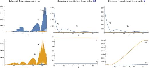
Comparison of errors |$\mathfrak {e}_l$| (see equation (B2)) for different boundary conditions. We convert our original DAEs (164) and (165) into ODEs which mathematica is capable of solving by differentiating the latter equation, giving equation (174). The left-hand plots show the result of substituting the obtained solution back into (164) and (174); this is merely a consistency check of mathematica’s algorithm, and the resulting error is predictably small (regardless of which set of boundary conditions we use). We then solve (164) and (174) together with a naïve set of boundary conditions (Table B1) that do not contain information about the original DAEs. We substitute the solution obtained with these boundary conditions back into the original DAEs (164) and (165), and show the resulting error in the central plots. For the lower ones of these plots, corresponding to the equation that was differentiated, a large, constant error can be seen. This reflects the fact that a solution to (174) will typically differ by some integration constant from a solution of the original equation (165). To fix this constant at the correct value (of zero), we need to use the more careful boundary conditions of Table 2. With these, as shown in the right-hand plots, the error becomes small.
If we had not worried about fixing the integration constant correctly, we might instead have adopted a set of boundary conditions like those of Table B1, which are natural-looking ones to use to ensure that solutions are well behaved at the centre and do not give rise to a current sheet at the outer boundary. Fig. B1 clearly shows that the resulting solutions fail to satisfy the original DAE system.
| m | Centre | Crust–core boundary |
|---|---|---|
| |$\bar{U}^{\prime }_2(0) = 0$| | |$R_{\rm out}\bar{U}^{\prime }_2(R_{\rm out})+4\bar{U}_2(R_{\rm out}) = 0$| | |
| 1 | |$\bar{U}_4^{\prime }(0) = 0$| | |$R_{\rm out}\bar{U}^{\prime }_4(R_{\rm out})+6\bar{U}_4(R_{\rm out}) = 0$| |
| X1(Rout) = 0 | ||
| X3(Rout) = 0 | ||
| |$\bar{U}^{\prime }_2(0) = 0$| | |$R_{\rm out}\bar{U}^{\prime }_2(R_{\rm out})+4\bar{U}_2(R_{\rm out}) = 0$| | |
| 2 | |$\bar{U}_4^{\prime }(0) = 0$| | |$R_{\rm out}\bar{U}^{\prime }_4(R_{\rm out})+6\bar{U}_4(R_{\rm out}) = 0$| |
| – | ||
| X3(Rout) = 0 |
B2 Convergence
To prevent numerical errors at the centre, we evaluated some quantities at a small radial distance – given by equation (B1) – from their correct location. Our final check is to make sure that the introduced error is small, and converges to zero in the limit |$\mathfrak {d}\rightarrow 0$|; we do this in Fig. B2. Here we have used the correct boundary conditions, from Table 2; note that the large ‘integration constant’ error resulting from using the boundary conditions of Table B1 does not converge away as |$\mathfrak {d}\rightarrow 0$|.
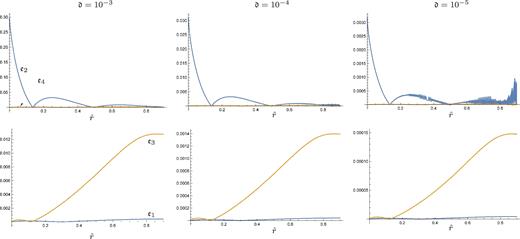
Convergence of the error in solutions as |$\mathfrak {d}\rightarrow 0$|. For |$\mathfrak {d} = 10^{-5}$|, the noisy inherent error present from mathematica’s solution becomes visible; i.e. the error introduced from evaluating quantities slightly away from the origin reduces to the level of intrinsic error from mathematica’s solution method. Note that the actual physical results for |$\bar{U}_l,X_l$| for these three values of |$\mathfrak {d}$| are indistinguishable.
