


Abstract
We analyse the radial pressure profiles, the intracluster medium (ICM) clumping factor and the Sunyaev–Zel'dovich (SZ) scaling relations of a sample of simulated galaxy clusters and groups identified in a set of hydrodynamical simulations based on an updated version of the treepm–SPH GADGET-3 code. Three different sets of simulations are performed: the first assumes non-radiative physics, the others include, among other processes, active galactic nucleus (AGN) and/or stellar feedback. Our results are analysed as a function of redshift, ICM physics, cluster mass and cluster cool-coreness or dynamical state. In general, the mean pressure profiles obtained for our sample of groups and clusters show a good agreement with X-ray and SZ observations. Simulated cool-core (CC) and non-cool-core (NCC) clusters also show a good match with real data. We obtain in all cases a small (if any) redshift evolution of the pressure profiles of massive clusters, at least back to z = 1. We find that the clumpiness of gas density and pressure increases with the distance from the cluster centre and with the dynamical activity. The inclusion of AGN feedback in our simulations generates values for the gas clumping (|$\sqrt{C}_{\rho }\sim 1.2$| at R200) in good agreement with recent observational estimates. The simulated YSZ–M scaling relations are in good accordance with several observed samples, especially for massive clusters. As for the scatter of these relations, we obtain a clear dependence on the cluster dynamical state, whereas this distinction is not so evident when looking at the subsamples of CC and NCC clusters.
1 INTRODUCTION
Galaxy clusters represent ideal systems for studies of both cosmology and astrophysics (e.g. Kravtsov & Borgani 2012; Planelles, Schleicher & Bykov 2016, for recent reviews). Although most of the total cluster mass is in the form of dark matter (DM; ∼85 per cent), they also contain a significant baryonic budget formed by the hot intracluster medium (ICM; ∼12 per cent) and the stellar component (∼3 per cent). Thanks to this particular composition, galaxy clusters can be observed in different wavebands, providing complementary observational probes to exploit their use as cosmological tools (e.g. Allen, Evrard & Mantz 2011).
The ICM, a hot ionized gas with typical temperatures of 107–108 K, emits strongly in the X-ray band via thermal Bremsstrahlung (Sarazin 1988). The resulting X-ray surface brightness depends quadratically on the electron number density ne. On the other hand, galaxy clusters can also be observed in the millimetre waveband via the thermal Sunyaev–Zel'dovich effect (SZ effect; Sunyaev & Zeldovich 1972). In this case, the observed signal depends on the dimensionless Compton-y parameter, which is proportional to the integral along the line of sight of the electron pressure (Pe ∝ neTe). Given their definitions, SZ and X-ray observations of galaxy clusters are differently sensitive to the details of the gas distribution and thermal state, thus allowing for complementary descriptions of the ICM thermodynamics. To exploit this connection, the ICM pressure distribution, directly connected to the depth of the cluster gravitational potential well and therefore to the total cluster mass, is a crucial quantity.
Both SZ observations and numerical simulations consistently show that the integrated SZ parameter, YSZ, is tightly related to cluster mass (Nagai 2006; Bonaldi et al. 2007; Bonamente et al. 2008; Battaglia et al. 2012a; Kay et al. 2012; Planck Collaboration XX 2014a; Le Brun et al. 2017). In particular, simulations indicate that, independently of the cluster dynamical state, the YSZ–M relation has a low scatter, with its normalization being only slightly dependent on the ICM physics. The X-ray analogue of YSZ, defined as the product of the gas mass and its X-ray temperature, i.e. YX ≡ Mgas · TX (Kravtsov, Vikhlinin & Nagai 2006), has also been shown to behave in a similar way (e.g. Nagai, Kravtsov & Vikhlinin 2007b; Fabjan et al. 2011; Planelles et al. 2014; Truong et al. 2016; Hahn et al. 2017). These two quantities relate to each other via the cluster thermal pressure distribution. Therefore, a detailed analysis of the ICM thermal pressure, and its dependencies on cluster mass, physics and redshift, are crucial to deepening our understanding of both ICM physics and cosmology.
The pressure structure of the ICM is sensitive to the combined action of gravitational and non-gravitational physical processes affecting galaxy clusters. Since these processes, acting on both galactic and cosmological scales, take place during the cluster evolution, the ICM is hardly ever in perfect hydrostatic equilibrium (HE; e.g. Rasia, Tormen & Moscardini 2004; Rasia et al. 2006; Nagai, Vikhlinin & Kravtsov 2007a; Gaspari et al. 2014; Biffi et al. 2016). The first observational constraints on cluster pressure profiles were provided by X-ray observations (e.g. Finoguenov et al. 2007; Arnaud et al. 2010). However, given their dependence on the square of the gas density, only extremely long exposures allow the observations of cluster outskirts (Simionescu et al. 2011; Urban et al. 2011, 2014). On the contrary, since SZ effect measurements depend linearly on the gas density and temperature, they are more suited to probe the external clusters regions (e.g. Basu et al. 2010; Plagge et al. 2010; Bonamente et al. 2012; Planck Collaboration V 2013c). Indeed, thanks to SZ facilities, such as the Planck telescope (Planck Collaboration XXIX 2014b; Bourdin, Mazzotta & Rasia 2015), the South Pole Telescope (SPT; Reichardt et al. 2013), the Atacama Cosmology Telescope (Hasselfield et al. 2013) or the Combined Array for Research in Millimeter-wave Astronomy (Plagge et al. 2013), the number and characterization of large SZ-selected cluster surveys has been dramatically improved in the recent past. From an observational point of view, however, constraining the outskirts of clusters is still challenging in either wavelengths because they require observations with high sensitivity: long exposures to detect low surface brightness and good angular resolution to remove contributions from point-like sources (e.g. Planck Collaboration X 2013d; Reiprich et al. 2013).
To date, X-ray and SZ observations of galaxy clusters together with results from numerical simulations (e.g. Borgani et al. 2004; Nagai et al. 2007b; Piffaretti & Valdarnini 2008) suggest that the ICM radial pressure distribution follows a nearly universal shape (e.g. Arnaud et al. 2010), at least out to R500 at z = 0. This universal pressure profile is well described by a generalized NFW model (GNFW; Zhao 1996; Nagai et al. 2007b), which is relatively insensitive to the details of the ICM physics. Beyond R500 the consistency of these results still needs to be confirmed since, besides the observational challenge, a number of processes (such as ongoing mergers and diffuse accretion, clumpy gas distribution, turbulent pressure support, e.g. Lau, Kravtsov & Nagai 2009; Vazza et al. 2009; Battaglia et al. 2010; Nagai & Lau 2011; Roncarelli et al. 2013; Vazza et al. 2013; Zhuravleva et al. 2013; Battaglia et al. 2015; Gaspari 2015; Gupta et al. 2016) contribute to deviate clusters from the idealized case of thermal pressure equilibrium in a smooth ICM distribution. As for the redshift evolution of the universal pressure profile, simulations predict no significant evolution outside of the cluster core (e.g. Battaglia et al. 2012a), a result that is confirmed by recent observations of high-redshift clusters (McDonald et al. 2014; Adam et al. 2015).
In order to explain possible deviations from a universal pressure profile, a detailed modelling of the gas density and pressure clumping from the core out to the cluster outskirts is of particular interest. Gas density and pressure clumpiness impact on X-ray and SZ effect measurements. For instance, gas inhomogeneities can bias high measurements of the gas density profiles (e.g. Mathiesen, Evrard & Mohr 1999; Nagai & Lau 2011), and induce as a consequence a flattening of the entropy profiles in cluster outskirts and a bias in gas masses and hydrostatic masses (e.g. Roncarelli et al. 2006; Nagai & Lau 2011; Simionescu et al. 2011; Eckert et al. 2013, 2015; Ettori et al. 2013a; Roncarelli et al. 2013). On the other hand, X-ray and SZ effect measurements are affected in different ways by gas density and pressure clumping. For instance, if the gas clumping is isobaric, the X-ray surface brightness will be augmented by a factor |$n_{\rm e}^{3/2}$|, whereas the SZ effect will not be altered. On the contrary, pressure clumping could affect significantly the SZ scaling relations and the cosmological implications derived from the analysis of the SZ power spectrum (e.g. Battaglia et al. 2015).
The aim of this paper is to perform a detailed analysis of the ICM thermal pressure distribution, the clumping factor and the SZ scaling relations of a sample of simulated galaxy clusters and groups that has been shown to produce a realistic diversity between cool-core (CC) and non-cool-core (NCC) systems (Rasia et al. 2015). Different cluster properties are analysed as a function of redshift, ICM physics, cluster mass, cluster dynamical state and cluster cool-coreness.
This paper is organized as follows. In Section 2, we briefly introduce the main characteristics of our simulated samples of galaxy clusters and groups. In Section 3, we analyse the radial pressure profiles of our sample of objects as a function of mass, dynamical state, redshift and physics included in our simulations. Section 4 shows results on the ICM clumping, both in density and pressure, whereas Section 5 shows the corresponding SZ scaling relations and their redshift evolution. Finally, in Section 6, we summarize our main results.
2 THE SIMULATIONS
2.1 The simulation code
We present the analysis of a set of hydrodynamic simulations of galaxy clusters performed with an upgraded version of the treepm–SPH code GADGET-3 (Springel 2005). The sample consists in zoomed-in simulations of 29 Lagrangian regions extracted from a parent N-body cosmological simulation (see Bonafede et al. 2011, for details on the initial conditions). The 29 regions have been identified around 24 massive DM haloes with M200 > 8 × 10¹⁴ h−1 M⊙ and 5 less massive systems with M200 = [1–4] × 1014 h−1 M⊙. As described in Planelles et al. (2014), each of the low-resolution regions has been re-simulated, with improved resolution and by including the baryonic component. The simulations consider a flat Λ cold dark matter cosmology with Ωm = 0.24, Ωb = 0.04, H0 = 72 km s−1 Mpc−1, ns = 0.96 and σ8 = 0.8. For the DM particles the mass resolution is mDM = 8.47 × 10⁸ h−1 M⊙, while the initial mass for the gas particles is mgas = 1.53 × 10⁸ h−1 M⊙. Gravity in the high-resolution region is calculated with a Plummer-equivalent softening length of ε = 3.75 h−1 kpc for DM and gas and ε = 2 h−1 kpc for black hole and stellar particles. The softening is kept fixed in comoving coordinates for all particles, except that, in the case of DM, it is given in physical units below z = 2.
For the hydrodynamical description, we use an updated formulation of smoothed particle hydrodynamics (SPH) as presented in Beck et al. (2016). This new SPH model has a number of features that improve its performance in contrast to standard SPH. These include higher order interpolation kernels and derivative operators as well as advanced formulations for artificial viscosity and thermal diffusion. With these improvements, we have performed three different sets of re-simulations characterized by different prescriptions for the physics of baryons:
NR. Non-radiative (NR) hydrodynamical simulations based on the improved SPH formulation presented in Beck et al. (2016).
CSF. Hydrodynamical simulations accounting for the effects of radiative cooling, star formation, SN feedback and metal enrichment, as already explained in Planelles et al. (2014). The chemical evolution model by Tornatore et al. (2007) is employed to account for stellar evolution and metal enrichment. Metal-dependent radiative cooling rates and the effects of a uniform UV/X-ray background emission are included according to the models by Wiersma, Schaye & Smith (2009) and Haardt & Madau (2001), respectively. Fifteen chemical species (H, He, C, Ca, O, N, Ne, Mg, S, Si, Fe, Na, Al, Ar, Ni) contribute to cooling. The star formation model is based on the original prescription by Springel & Hernquist (2003), where galactic outflows originated by SN explosions are characterized by a wind velocity of vw = 350 km s−1.
AGN. Hydrodynamical simulations accounting for identical physics as in the CSF case, plus active galactic nucleus (AGN) feedback. The sub-grid model for supermassive black hole (SMBH) accretion and AGN feedback employed in our simulations has been presented in Steinborn et al. (2015) and represents an improved version of the original model described in Springel, Di Matteo & Hernquist (2005). Here, mechanical outflows and radiation are combined and included in the form of thermal feedback. The efficiency of radiative and mechanical feedback depend on both the (Eddington-limited) gas accretion rate and the SMBH mass, providing a smooth transition between radio and quasar mode. We assume that a fraction εf = 0.05 of the radiative feedback couples to the surrounding gas as thermal feedback. In addition, the accretion is computed separately for hot and cold gas. In this work, we neglect hot gas accretion (αhot = 0) and consider only cold gas accretion, for which the Bondi accretion rate is boosted by a factor αcold = 100 (see Gaspari, Brighenti & Temi 2015). For further details on the model and its performance, we refer to the work by Steinborn et al. (2015).
The set of AGN simulations has been shown to generate, for the first time, a coexistence of CC and NCC simulated clusters with thermal and chemodynamical properties in good agreement with observations (see Rasia et al. 2015, for further details). This result is a consequence of the combined action of both the artificial conduction term included in the new hydro scheme and the new AGN feedback model, which improves the mixing capability of SPH and regulates the formation of stars in massive haloes.
2.2 The sample of simulated clusters
We identify groups and clusters in the high-resolution regions following a two-steps procedure. First, we run a friends-of-friends (FoF) algorithm with a linking length equal to 0.16 in units of the mean separation of the high-resolution DM particles. This step provides the centre of each halo, corresponding to the DM particle position within each FoF group with the minimum gravitational potential. Then, a spherical overdensity algorithm is applied to each halo and at each considered redshift in order to get the radius RΔ confining an average density equal to Δ times the corresponding critical cosmic density, ρc(z). In the following, we will refer to an overdensity Δ = 200, 500, 2500, or to the virial overdensity (Bryan & Norman 1998).
Following this procedure, we identify, within each of our three sets of re–simulations, a sample of ∼100 clusters and groups with M500 > 3 × 10¹³ h−1 M⊙ at z = 0. In the following, depending on the property to be analysed, we will either refer to the reduced sample of 29 central haloes (formed by 24 clusters with masses 4 × 10¹⁴ h−1 M⊙ ≤ M500 ≤ 2 × 10¹⁵ h−1 M⊙ and 5 isolated groups with 6 × 10¹³ h−1 M⊙ ≤ M500 ≤ 3 × 10¹⁴ h−1 M⊙ at z = 0) or to the complete sample of ∼100 systems (formed by all the haloes found within each region in addition to the central one). In general, we will use the reduced sample of groups and clusters throughout the paper, whereas the whole sample will be employed in the analysis of the scaling relations.
Based on different cluster properties, we have considered two different classifications for the groups and clusters belonging to the reduced sample in our AGN simulations:
CC-like and NCC-like haloes. Following the criteria presented in Rasia et al. (2015), we classify our systems in the AGN simulations according to their core thermodynamical properties. In particular, those systems with a central entropy K0 < 60 keV cm2 and a pseudo-entropy σ < 0.55 are defined as CCs; those systems not satisfying these conditions are instead considered as NCC objects. With this criterion, 11 out of 29 haloes are classified as CC clusters. As described in Rasia et al. (2015), the entropy and metallicity profiles of simulated CC and NCC objects are in good agreement with observations of these two cluster populations.
Regular and disturbed haloes. Groups and clusters are classified according to their global dynamical state. In order to do so, we combined two different methods generally used in simulations (e.g. Neto et al. 2007; Meneghetti et al. 2014): (a) the centre shift, given by the offset between the position of the cluster minimum potential and its centre of mass in units of its virial radius (e.g. Crone, Evrard & Richstone 1996; Thomas et al. 1998; Power, Knebe & Knollmann 2012), that is, δr = ||rmin − rcm||/Rvir and (b) the mass fraction contributed by substructures, that is, fsub = Msub/Mtot, where Msub and Mtot are, respectively, the total mass in substructures and the total mass of a given system as provided by subfind (Springel et al. 2001; Dolag et al. 2009). We consider a system to be regular when δr < 0.07 and fsub < 0.1, whereas those systems with larger values for δr and fsub are labelled as disturbed. Clusters for which both criteria are not concurrently satisfied are considered as intermediate cases. Following this classification we end up with 6 regular, 8 disturbed and 15 intermediate systems (see also Biffi et al. 2016).
3 PRESSURE PROFILES
3.1 Scaled pressure profiles
Fig. 1 shows the individual scaled pressure profiles (green dotted lines) out to 4 × R500 at z = 0 for the reduced sample of systems in the NR, CSF and AGN simulations, respectively. The mean scaled pressure profile derived in each case is shown by a thick line together with 1σ scatter around it (streaky area). Independently of the physics included in our simulations, and despite the existence of some outliers, individual dimensionless pressure profiles follow a nearly universal shape with a relatively small scatter around the average, especially at intermediate radii, 0.3 ≲ r/R500 ≲ 1, where we obtain a mean scatter of ∼11 per cent. This result is in agreement with the characteristic cluster-to-cluster dispersion at intermediate radii obtained for the pressure profiles derived for both observed (∼10–40 per cent; e.g. Arnaud et al. 2010; Sun et al. 2011) and simulated clusters (e.g. Borgani et al. 2004; Nagai et al. 2007b). Deviations from the self-similar behaviour, mainly apparent in inner (r ≤ 0.3R500) and outer clusters regions (r ≥ R500), result from the combination of a number of factors, such as, the effect of different feedback processes or the particular gas distribution and dynamical structure of the considered systems. Indeed, whereas the scatter in central regions (r ≲ 0.2/R500) is larger (by a factor of ∼1.5) in the AGN case, the fact that the three models show a similar scatter at larger radii indicates that the different formation histories of individual systems may also play a significant role. As we will discuss in Section 5, given the relation between YX and YSZ and the obvious connection between cluster mass and pressure, this low scatter explains why the YX–M relation is usually observed to be a good proxy for mass (e.g. Kravtsov et al. 2006; Fabjan et al. 2011; Planelles et al. 2014).
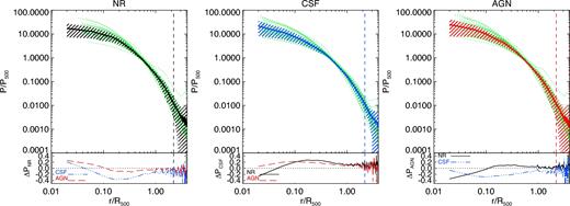
Individual P/P500 pressure profiles (green dotted lines) out to 4R500 at z = 0 for our sample of 29 central groups and clusters in the NR, CSF and AGN simulations (panels from left to right, respectively). In each panel, the continuous thick line represents the corresponding mean profile of each sample, whereas the streaky area stands for 1σ scatter around the mean. The vertical line marks the mean value of Rvir, in units of R500, within each sample. The relative difference between the mean profiles obtained for the reference model in each panel and the other two models is shown in the bottom panels as ΔPREF = (Pmean − PREF)/Pmean.
In order to highlight the differences between the mean pressure profiles obtained for each model, we show in the bottom panels of Fig. 1 their relative difference computed as ΔPREF = (Pmean − PREF)/Pmean, where PREF stands for the reference model in each panel (i.e. from left to right, NR, CSF and AGN) and Pmean stands for the other two models in comparison. From these panels it is clear that, for r ≲ 0.1R500, the AGN model produces the higher central pressure (by ∼20–30 per cent) while it is more similar to the NR run than to the CSF at larger radii.
We have checked that the mean and the median radial profiles of our sample of clusters are very similar to each other. Therefore, in order to compare with observational data and unless otherwise stated, in the following we will use the mean simulated profiles shown in Fig. 1.
3.2 Comparison with observational samples
In this section, we will compare our simulated data with five different observational samples briefly described as follows.
Arnaud et al. (2010) presented the analysis of the pressure profiles of the REXCESS sample (Böhringer et al. 2007), a selection of 33 nearby (z < 0.2) clusters within a mass range of 1014 M⊙ < M500 < 1015 M⊙ observed with XMM–Newton. They derived a universal pressure profile out to cluster edges by combining observations within the radial range [0.03–1]R500 with results from numerical simulations within [1–4]R500. According to the criteria defined in Pratt et al. (2009), they divided this sample of clusters in CC (those with peaked density profiles in central regions) and morphologically disturbed (those with a large centre shift parameter) systems. The mass M500 of each cluster was estimated using the M500–YX scaling relation as obtained by Arnaud, Pointecouteau & Pratt (2007).
Planck Collaboration V (2013c) analysed the SZ pressure profiles of a sample of 62 local (z < 0.5) massive clusters with 2 × 10¹⁴ M⊙ < M500 < 2 × 10¹⁵ M⊙, identified from the Planck all-sky survey. These SZ-selected systems, taken from the Planck early SZ sample (Planck Collaboration VIII 2011a), have been also followed-up with XMM–Newton observations. The radial SZ effect signal of this sample of clusters was detected out to 3R500. In order to provide a proper radial analysis, they combined this data with XMM–Newton observed profiles within [0.1–1]R500. Masses and radii of these clusters were derived by means of the YX–M500 relation by Arnaud et al. (2010). Following the classification criterion described in Planck Collaboration XI (2011b), they divided the whole sample of clusters in 22 CC and 40 NCC systems.
Sayers et al. (2013) analysed the pressure profiles of a sample of 45 galaxy clusters, with a median mass of M500 = 9 × 10¹⁴ M⊙, within a redshift range of 0.15 ≲ z ≲ 0.89. Total masses were derived using the gas mass as a proxy (see Mantz et al. 2010, for details). These clusters, imaged by means of SZ observations with the Bolocam at the Caltech Submillimeter Observatory, span a radial range within [0.07–3.5]R500. The whole sample of clusters is formed by 17 CC clusters (defined according to their X-ray luminosity ratio), 16 disturbed objects (defined according to their X-ray centroid shift) and 2 systems that are disturbed and have a CC.
McDonald et al. (2014) presented the X-ray analysis of a sample of 80 galaxy clusters from the 2500 deg2 SPT survey. The masses of the systems, with M500 ≳ 3 × 10¹⁴E(z)− 1 M⊙, were derived using the YX–M relation by Vikhlinin et al. (2009). Assuming a self-similar temperature profile, they made an X-ray fit to their clusters, which were divided in different subsamples according to their redshift and central densities. In this way, they constrained the shape and evolution of the temperature, entropy and pressure radial profiles within 1.5R500 and out to z = 1.2.
As for the observation of smaller systems, Sun et al. (2009, 2011) analysed Chandra archival data for 43 nearby (0.012 < z < 0.12) galaxy groups with M500 = 1013–1014 h−1 M⊙. They obtained gas properties out to at least R2500 for the whole sample and out to R500 for 11 groups. For an additional subsample of 12 groups, they extrapolated to derive properties at R500.
It is important to note the diversity of these sets of observations both in their nature (i.e. X-rays combined with simulations, X-rays or SZ observations) and in the properties of the considered cluster/group samples. In addition, there is also a difference in the criteria used to classify the observed clusters in CC and NCC systems. Given the diversity of these observational samples, the comparison with the pressure profiles of our simulated systems will help us to provide a more robust analysis of the existing dependencies on cluster mass, redshift and dynamical state.
We note that, when cluster masses are derived assuming HE, as it is done in most X-ray analyses, they are underestimated by a factor ∼10–20 per cent (e.g. Arnaud et al. 2010). In order to compare simulated and observed pressure profiles, given the dependencies of P500 and R500 on mass, the hydrostatic mass bias would imply a reduction in these quantities, translating therefore the scaled profiles. Since the change induced by this bias is relatively small (e.g. a 15 per cent mass bias implies a ∼10 per cent change in P/P500 and ∼5 per cent in R500; Planck Collaboration V 2013c), given that its magnitude is still uncertain, we decide not to account for this correction and refer the reader to more detailed analyses that specifically address the issue of HE (e.g. Biffi et al. 2016, and references therein).
In addition, the definition of P500 given by equation (2) reflects the variation of the pressure within R500 with mass and redshift as predicted by the standard self-similar model. Unlike Arnaud et al. (2010) or Planck Collaboration V (2013c), but in a similar way to Sayers et al. (2013), we do not include any additional correction to the mass dependence of P500 (see equations 7 and 8 of Arnaud et al. 2010). We have checked that, for the sample of AGN systems considered here, the M500–YX, 500 scaling relation is self-similar out to redshift 1 and therefore there is no need to introduce any additional non-self-similar mass dependence (as shown in Truong et al. 2016, a similar result is also obtained for our complete set of systems in our three models).
3.2.1 Dependence on cluster mass and physics included
The left-hand and right-hand panels of Fig. 2 show, respectively, the mean pressure profiles P/P500, scaled by (r/R500)3, for the sample of 24 central clusters and 5 central groups within each of our simulations. We compare these mean profiles with different observational samples of groups and clusters. For completeness, we also compare with the universal pressure profile obtained by Arnaud et al. (2010). The relative difference between the mean simulated profiles and the best fit to a GNFW model by Arnaud et al. (2010) is shown in the bottom panels as ΔPGNFW = (Pmean − Pfit)/Pmean.
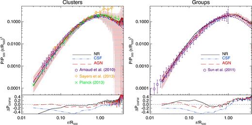
Mean P/P500 pressure profiles, weighted by (r/R500)3, out to 4 × R500 at z = 0 for our sample of 24 central clusters (left-hand panel) and 5 central groups (right-hand panel). Black, blue and red lines stand for the mean profiles in the NR, CSF and AGN simulations, respectively. For the sake of clarity, the streaky red area shows 1σ deviation around the mean profile in the AGN run. Observed pressure profiles from Arnaud et al. (2010), Sun et al. (2011), Planck Collaboration V (2013c) and Sayers et al. (2013) are used for comparison (different symbols with error bars). The purple dotted line shown in both panels corresponds to the best-fitting profile to a GNFW model as obtained by Arnaud et al. (2010) (see Section 3.4 for further details). The relative difference between the simulated profiles and the best-fitting profile of Arnaud et al. (2010) is shown in the bottom panels.
We focus first on the analysis of the pressure profiles of massive clusters and their dependencies on the different physical models included in our simulations (left-hand panel of Fig. 2). In general, simulated and observed profiles show a good agreement (within 1σ) and a considerably small scatter at intermediate cluster radii (0.2 ≲ r/R500 ≲ 1), indicating that they are nearly self-similar in this radial range. Within inner regions, the AGN simulations tend to produce a slightly higher central pressure (by a factor ∼1.2–1.5) than the other two models, whereas the NR runs produce the lowest values. Nevertheless, all our simulated sets tend to produce results that are close to each other and in remarkably good agreement with observations, especially to those from the REXCESS sample (Arnaud et al. 2010). Despite the consistency with the data, the dispersion of the profiles in these internal regions is relatively large, presumably due to both the different formation histories and the different effects that radiative cooling and AGN feedback play on the ICM thermal properties. Indeed, thanks to the improved SPH scheme employed in our simulations, the NR model produces a lower central pressure in clusters and a smoother thermal distribution than the standard SPH. Quite interestingly, the combination of the new hydro scheme and the AGN feedback model, allows the AGN simulations to efficiently compensate overcooling and to keep pressurized a large amount of low-entropy gas that now remains in the hot phase, providing therefore a higher pressure in the centre. In outer cluster regions (r ≳ R500), however, our three simulation sets produce quite similar (within a few per cent) mean profiles and the scatter between them is slightly reduced. The dispersion around the mean profiles is however larger as a result of the additional matter and dynamical activity characterizing these external cluster regions. In general, even when the agreement with the observed profiles is quite encouraging, simulated profiles are in better agreement with the observed SZ mean profile from Planck Collaboration V (2013c), showing as well a larger cluster-to-cluster scatter than at intermediate regions. In these outer regions, in agreement with previous studies (e.g. Battaglia et al. 2010), our mean profiles are systematically higher (by ∼20 per cent) than the universal profile presented in Arnaud et al. (2010). Nevertheless, we would like to point out that we perfectly reproduce the outer part of the profile given by Arnaud et al. (2010) when we restrict our sample to the ∼20 most massive clusters with M500 ≥ 6 × 10¹⁴ h−1 M⊙.
To further investigate the impact of the different physical models on systems of different masses, we focus now on the analysis of groups (right-hand panel of Fig. 2). The combined action of different feedback processes on systems of different masses is expected to affect in a different way the distribution of pressure within the considered systems, both in the core and in the outskirts. In our case, however, independently of the physics included, groups and clusters show very similar mean pressure profiles, suggesting that they are nearly self-similar in all models. This result seems to be in contradiction with the effect seen in recent simulations (e.g. Battaglia et al. 2010; McCarthy et al. 2014), where the pressure profiles of groups within radiative simulations are lower (higher) in central (outer) regions than in more massive clusters, being in line with the expectation that feedback is more efficient in the central regions of low-mass systems. Again, this apparent contradiction disappears by selecting a sample of lower mass groups. Indeed, if we use our whole sample of systems (not only the 29 central objects), we can set a lower mass threshold for the sample of groups, that is, we can consider all the systems with 3.0 × 10¹³ h−1 M⊙ ≤ M500 < 3.0 × 10¹⁴ h−1 M⊙. For this larger sample of smaller groups, formed by more than 70 systems with a mean mass 〈M500〉 ∼ 8.2 × 10¹³ h−1 M⊙ (a lower value than the mean mass of our sample of five isolated groups, that is, 〈M500〉 ∼ 1.9 × 10¹⁴ h−1 M⊙), both of our radiative simulations produce, at r ≲ r500, a significant decrease of the pressure with respect to the NR case (as an example, at r = 0.1R500, the CSF and AGN models show a pressure lower by a factor of ∼2 and 2.7, respectively, than the NR run). This reduction of the central pressure induced by AGN feedback at the scale of groups is in broad agreement with previous simulated results considering a similar range of masses (e.g. McCarthy et al. 2014). Contrarily, this effect is not so pronounced for a larger sample of high-mass systems (a sample of more than 30 clusters with M500 ≥ 3.0 × 10¹⁴E(z)−1 M⊙ and 〈M500〉 ∼ 7.7 × 10¹⁴ h−1 M⊙) for which the central pressure seems to be quite insensitive to the inclusion of AGN feedback since both CSF and AGN simulations produce very similar profiles. This result, in agreement with recent findings from simulations (e.g. McCarthy et al. 2014; Pike et al. 2014; Planelles et al. 2014), is also in line with the expectation that the total thermal content of the ICM is only weakly affected by feedback sources in massive systems while being more sensitive to feedback in less massive objects (e.g. Gaspari et al. 2014). In any case, it is important to point out that the inclusion of AGN feedback in our simulations produces pressure profiles in galaxy groups that are in good agreement (within ∼15–20 per cent) with the observations reported by Sun et al. (2011) and with the universal fit of Arnaud et al. (2010).
As for the outskirts of groups and clusters the mean pattern is also quite similar. However, in the case of clusters, the scatter increases progressively with radius being much larger than in groups. This increase in outer regions is partially associated with the fact that, whereas our sample of clusters is formed by 24 non-isolated massive systems, our sample of groups is composed by 5 isolated objects. Indeed, in the case of groups, the dispersion around the mean profile is quite sensitive to the group selection, not only in terms of mass but also depending on the environment where groups reside: when we consider our larger sample of non-isolated groups, the dispersion also increases significantly in the outermost regions. In addition, there should be also a contribution from the infall of pressurized clumps or by gas in filaments or stripped from merging haloes. As we will discuss below, this is consistent with the higher degree of clumpiness observed in the peripheral regions of massive clusters. Moreover, as suggested by recent studies (Avestruz, Nagai & Lau 2016), non-thermal pressure, associated with gas motions in outer cluster regions, plays a major role in the ICM thermal evolution and therefore it can also affect the distribution of thermal pressure.
3.2.2 Dependence on cool-coreness
Fig. 3 shows the mean pressure profiles P/P500 obtained for the subsamples of CC (left-hand panel) and NCC (right-hand panel) clusters at z = 0 within our AGN simulations. In order to compare with observations, the de-projected pressure profiles of the disturbed and CC clusters of the BOXSZ sample, as derived by Sayers et al. (2013), together with those derived by McDonald et al. (2014) for a sample of 80-SPT selected clusters are also shown. We note that these observed profiles are not exactly at z = 0 but at a median redshift of 0.42 in the case of Sayers et al. (2013) and at 0.3 < z < 0.6 in the case of McDonald et al. (2014).1 However, as we will discuss in Section 3.3, since cluster pressure profiles do not show a noticeable z-evolution, we can perform this comparison. Moreover, we remind that, given the different criteria used to classify clusters in CC/NCC, this comparison has to be intended as a qualitative approach to emphasize the similarity between the trend of the two classes.
![Mean radial profiles of scaled pressure, P/P500, out to 4R500 at z = 0 for our CC (left-hand panel) and NCC (right-hand panel) clusters within our AGN simulations. Individual profiles are shown with thin dotted black lines. The mean profile of each sample is represented instead by a continuous red line surrounded by a shaded area representing 1σ scatter around the mean profile. The average pressure profiles of observed CC and NCC clusters as derived by Sayers et al. (2013) (purple open circles with error bars) and McDonald et al. (2014) (green open circles with error bars) are used for comparison. In the bottom panels, we show the relative difference between the mean profiles of CC and NCC clusters as obtained in all the samples. In particular, ΔPCC = [(P/P500)CC − (P/P500)NCC]/(P/P500)CC (ΔPNCC is computed in a similar way). The horizontal dotted line marks a zero relative difference.](https://oup.silverchair-cdn.com/oup/backfile/Content_public/Journal/mnras/467/4/10.1093_mnras_stx318/1/m_stx318fig3.jpeg?Expires=1750609731&Signature=wVjUNkcMEF4Xa9r0hfQCNHGyTF99Wpy2MS-uIHOMIx9qr-m-jbwMkz14B2ZLUDPrAJoe5wvux-sh9lbt0dty18Z-DSw-wrVGQCLEz19MXcEmeW0eRPvX8MS3wq4qBvSDmTxQIIQE0O1HY1Tfurv4pEnBU5yt24zewueVmuRJeMQyB7pMzzck5Aa-Kku7AYAgNRX97eyQK4D94NJV5XEOermWyJpxCwvqeU5PZzYLICHwaaWxgZ0KmI6LlEdep-r-ZwpbZFk7FUTQ4Dt-mLFDfzjF3JZhp3rQw7UDtcVZxiZZdGNA9d-ct8YClofpLWa96XGii5QXp72R4gsp3NirAQ__&Key-Pair-Id=APKAIE5G5CRDK6RD3PGA)
Mean radial profiles of scaled pressure, P/P500, out to 4R500 at z = 0 for our CC (left-hand panel) and NCC (right-hand panel) clusters within our AGN simulations. Individual profiles are shown with thin dotted black lines. The mean profile of each sample is represented instead by a continuous red line surrounded by a shaded area representing 1σ scatter around the mean profile. The average pressure profiles of observed CC and NCC clusters as derived by Sayers et al. (2013) (purple open circles with error bars) and McDonald et al. (2014) (green open circles with error bars) are used for comparison. In the bottom panels, we show the relative difference between the mean profiles of CC and NCC clusters as obtained in all the samples. In particular, ΔPCC = [(P/P500)CC − (P/P500)NCC]/(P/P500)CC (ΔPNCC is computed in a similar way). The horizontal dotted line marks a zero relative difference.
As shown in the bottom panels of Fig. 3, the mean profiles we obtain for the CC/NCC cluster populations are in good agreement with each other at intermediate (0.2R500 < r < R500) radii. This is consistent with the work by Rasia et al. (2015) as well as with a number of observational results (e.g. Arnaud et al. 2010; Planck Collaboration V 2013c). However, as expected, these profiles clearly diverge from each other in inner cluster regions (r/R500 ≲ 0.2), where observations generally report slightly higher values of pressure and steeper profiles in CC than in NCC clusters. The mean values of the core pressure and the shape of the profiles obtained for our samples of CC and NCC systems are in good agreement with the observational trend (at the innermost radius, our CC clusters show a mean pressure ∼2.5 times higher than our NCC clusters). In general, our results for these two cluster populations show a good consistency (within 1σ) with the observations by Sayers et al. (2013), especially in inner cluster regions. However, especially for NCC systems, our mean pressure profile in cluster outskirts (r > R500) is lower (e.g. at r = 3R500 by a factor of ∼7) than the one reported by Sayers et al. (2013), being in better agreement with the observational determinations by Arnaud et al. (2010) or Planck Collaboration V (2013c) (see Sayers et al. 2013 or McDonald et al. 2014, for a more detailed discussion).
Fig. 3 also shows that the mean profile obtained for our sample of NCC objects has a higher dispersion, especially in the outer regions, than for the sample of CC clusters. The same happens between the different observational samples used for comparison. As we will discuss in Section 4, the larger dispersion in cluster outskirts is mostly produced by a clumpier gas distribution in outer regions of unrelaxed massive galaxy clusters. In addition, as we will also see in Section 5, small changes in the pressure profiles depending on either the dynamical state or the cool-coreness of the considered systems have a different impact on the corresponding YSZ–M relation (see Table 2).
3.3 Evolution with redshift
Thanks to its redshift independence, the SZ effect provides the ideal means to trace the evolution of the ICM properties, especially in the outer cluster regions. The young dynamical age of these regions make them quite interesting to trace the recent history of cluster assembly. However, they are hardly accessible to X-ray observations of distant clusters because of surface brightness dimming.
Fig. 4 shows the mean pressure profiles obtained for our sample of 29 central systems at z = 0.5 and z = 0.8 within each of our three sets of simulations. To compare with observational data, we use the high-redshift (〈z〉 = 0.82) and low-redshift (〈z〉 = 0.46) pressure profiles from the SPT sample presented in McDonald et al. (2014). Despite the differences in mass of the samples in this comparison, independently of the considered redshift and physical model, we obtain a relatively good agreement with the observational data throughout the radial range. The major differences arise at r ≤ 0.3R500, where the CSF model shows the best agreement (within 1σ at both redshifts) with the data. In particular, simulations predict gas pressure in excess of the observed one in core regions, r ≤ 0.1R500, with the NR and AGN models showing the largest deviations (by ∼3σ and ∼2.5σ, respectively) from the data at z = 0.8. Simulations are more consistent with the observed values at intermediate radii, 0.1 ≤ r/R500 ≤ 0.3, where, again, the NR and AGN runs show the largest deviation (by ∼2.5σ and ∼2σ, respectively) from the high-redshift data. We note that part of the discrepancy in the normalization is due to the fact of comparing with the data by McDonald et al. (2014), since it shows lower pressure values than the rest of observational samples we have used for comparison (see Figs 2 and 3). However, if we focus on the z-evolution, simulated and observed profiles show a similar trend. Interestingly, if we compare with the NR model, including AGN physics slightly increases the central pressure at both redshifts. This is due to the effect that AGN feedback and thermal conduction have in pressurizing the gas in cluster cores. The agreement with observations improves, for all the three models, in outer regions, i.e. at r ≥ 0.3R500, being particularly encouraging at z = 0.5, whereas at z = 0.8 there are more apparent deviations. In any case, in these external regions, observed and simulated profiles are consistent within 1σ with each other.
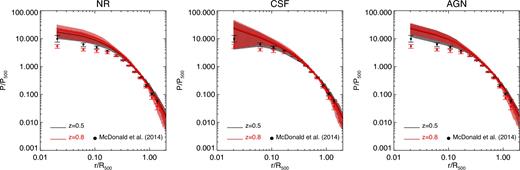
Mean pressure profiles for our sample of 29 main groups and clusters at z = 0.5 (black line) and at z = 0.8 (red line) within the NR (left-hand panel), CSF (middle panel) and AGN (right-hand panel) simulations. Coloured regions in black and red represent, respectively, 1σ scatter around the mean profiles at z = 0.5 and at z = 0.8. Filled circles with error bars refer to the observational sample by McDonald et al. (2014) at a mean redshift of 0.46 (black) and 0.82 (red).
As pointed it out by McDonald et al. (2014), from the analysis of the pressure profiles at z = 0.8, we see that both observed and simulated profiles show a small but measurable steepening in outer regions. This steepening can be due to the existence of dense gas clumps which would tend to increase both the pressure measurements and the scatter around the mean universal profile. Moreover, the lower pressure that characterizes the outskirts at higher redshifts may indicate a delayed effect of heating sources.
Overall, simulated and observed scaled pressure profiles show little (if any) redshift evolution. This lack of evolution suggests that any non-gravitational processes should have played an action on ICM pressure at even earlier epochs. As shown in McDonald et al. (2014), our results on the evolution of pressure profiles are also broadly consistent with previous simulations (e.g. Battaglia et al. 2012a) as well as with additional observations of high-redshift clusters (e.g. Adam et al. 2015).
3.4 Universality of pressure profiles
To analyse the consistency of the mean pressure profiles obtained in our simulations, we perform a Monte Carlo Markov Chain (MCMC) analysis to determine the values of the parameters describing the GNFW model of equation (3). We have performed this analysis for different sets of fixed and free parameters. In particular, in order to compare with different observational samples, we have considered two specific cases: two four-parameters models where we have fixed in each case γ and β, respectively. Therefore, we assume a first four-parameters model with [P0, c500, α, β] left free and γ fixed to 0.31, in accordance to the best-fitting value obtained by Arnaud et al. (2010), and a second four-parameters model described by leaving [P0, c500, γ, α] free and β fixed to 5.0, which is an intermediate value to those obtained by Arnaud et al. (2010) and Planck Collaboration V (2013c). We carried out our analysis by considering the subset of 24 massive simulated clusters, as well as the subsamples of CC and NCC systems within them. The best-fitting parameters we obtain for each of the considered cases are shown in Table 1. In all cases, we have performed the analysis within the radial range 0.02 ≲ r/R500 ≲ 4.
Values of the best-fitting parameters describing the GNFW pressure profile given by equation (3) for different sets of fixed parameters (indicated with a). Results are shown for our sample of 24 massive clusters in the NR, CSF and AGN simulations. Results obtained for the subsamples of CC and NCC systems within the AGN model are also shown. Fitted parameters in each case are shown with errors representing 1σ uncertainty.
| Simulation | Sample | z | P0 | c500 | γ | α | β |
|---|---|---|---|---|---|---|---|
| NR | Reduced | 0.0 | 6.85 ± 1.64 | 1.09 ± 0.50 | 0.31a | 1.07 ± 0.28 | 5.46 ± 1.15 |
| CSF | Reduced | 0.0 | 6.35 ± 1.89 | 0.63 ± 0.52 | 0.31a | 0.86 ± 0.24 | 6.73 ± 1.54 |
| AGN | Reduced | 0.0 | 8.25 ± 2.90 | 0.54 ± 0.54 | 0.31a | 0.81 ± 0.22 | 7.32 ± 1.91 |
| Reduced-CC | 0.0 | 11.96 ± 3.59 | 0.64 ± 0.44 | 0.31a | 0.81 ± 0.16 | 7.06 ± 1.72 | |
| Reduced-NCC | 0.0 | 5.71 ± 1.45 | 0.71 ± 0.55 | 0.31a | 0.93 ± 0.22 | 6.34 ± 2.14 | |
| Reduced | 0.0 | 3.99 ± 5.84 | 1.19 ± 0.14 | 0.52 ± 0.22 | 1.17 ± 0.15 | 5.0a | |
| 0.25 | 2.72 ± 6.16 | 0.98 ± 0.12 | 0.63 ± 0.21 | 1.12 ± 0.13 | 5.0a | ||
| 0.5 | 3.46 ± 6.06 | 1.07 ± 0.12 | 0.54 ± 0.21 | 1.12 ± 0.15 | 5.0a | ||
| 0.8 | 15.34 ± 6.16 | 1.39 ± 0.12 | 0.18 ± 0.17 | 0.92 ± 0.12 | 5.0a | ||
| 1.0 | 24.19 ± 5.28 | 1.24 ± 0.08 | 0.14 ± 0.12 | 0.77 ± 0.04 | 5.0a |
At z = 0, the results of our fittings are in broad agreement with the values obtained from previous observational analyses. In the case with γ = 0.31, as it is shown in Fig. 5, the best-fitting values obtained for the AGN run show a good consistency (within 1σ) with the best fits obtained by Arnaud et al. (2010), whereas the comparison is slightly worse when looking at the Planck Collaboration V (2013c) best-fitting values. In this case, however, when we include AGN physics, we obtain for the outer slope β a higher value than the one reported by Arnaud et al. (2010) (derived from early simulations by Borgani et al. 2004; Nagai et al. 2007a; Piffaretti & Valdarnini 2008), whereas our NR model produces a better match. This higher value of the outer slope is in disagreement with the trend obtained by recent simulations accounting for AGN feedback (e.g. Greco et al. 2015; Le Brun, McCarthy & Melin 2015) or with more recent Planck Collaboration V (2013c) data, which, as shown in Fig. 5, tend to obtain lower values of β than reported by Arnaud et al. (2010). Our results on the outer slope are however in better agreement with recent observational estimates by Ramos-Ceja et al. (2015) (β ∼ 6.35) or Sayers et al. (2016) (β ∼ 6.13). Given the degeneracies between the different parameters in this model, it is difficult to perform a direct and reliable comparison between the best-fitting values obtained from different studies. However, we note from Fig. 5 that, whenever there is a well-defined degeneracy direction between a pair of parameters, both data and simulations tend to lie on this direction, with no significant offset. Therefore, small effects related, e.g. to the radial range covered by observations and by simulations or residual mass differences, could cause this tension in the values of the fitting parameters.
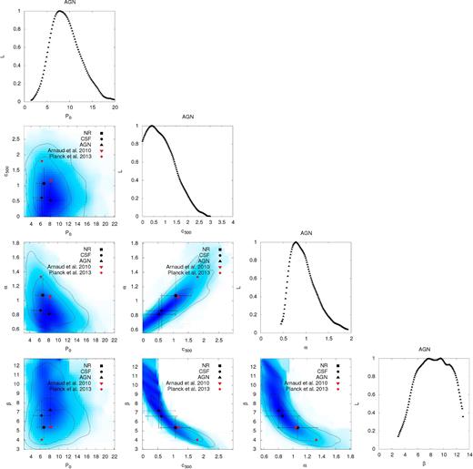
Likelihood confidence regions for the parameters of the GNFW model with γ = 0.31 obtained for the sample of clusters within our AGN simulations. Solid lines on the 2D distributions represent the 68 and 95 per cent confidence levels. Filled symbols in black (squares, circles and triangles, respectively) mark the best-fitting values obtained for the NR, CSF and AGN runs, whereas red symbols are for the best-fitting values obtained by Arnaud et al. (2010) and Planck Collaboration V (2013c).
As for the population of CC and NCC clusters within our AGN simulations at z = 0, the diversity of their corresponding mean profiles is more evident from the values of the best-fitting parameters than from the mean profiles shown in Fig. 3. Indeed, as obtained in previous observational studies (e.g. Planck Collaboration V 2013c), the mean profiles derived for CC/NCC systems show the largest discrepancy in the normalization, with CC having larger values of P0 than NCC clusters. In general, the broad agreement obtained between observed and simulated pressure profiles from the core (with a clear distinction between CC and NCC systems) out to cluster outskirts, suggests that the thermal structure of cluster cores is responsible for the scatter and shape of the mean profiles in central regions, while additional factors, such as the overall dynamical state, determine the behaviour in the cluster outskirts. The poor observational characterization of the peripheral regions and the increasing importance of the non-thermal pressure support, call for the need of a deeper understanding of the physics and distribution of the gas in these regions (e.g. Avestruz et al. 2015, 2016), both from observations and from simulations.
For completeness, we show in Fig. 6 the mean pressure profiles obtained for our sample of massive clusters in the AGN simulations at z = 0.0, 0.25, 0.5, 0.8, 1. The bottom panel of this figure shows ΔPGNFW, that is the relative difference between the mean profile obtained at each redshift and the corresponding best fit to the GNFW model when we consider β = 5. In general, our best-fitting models recover quite well the mean profiles at different redshifts. For the AGN simulations, the scatter between the recovered and the input profiles is quite small (≲5 per cent) at all redshifts for 0.03R500 ≲ r ≲ r500, while it increases considerably in outer regions and especially at higher redshift. A similar result is also obtained for the sample of clusters in the NR and CSF simulations. If we compare our fitting parameters to the results obtained by McDonald et al. (2014) for a sample of clusters at z < 0.6 and z > 0.6, we obtain a broad agreement, especially at lower redshifts. However, given the obvious discrepancies between the different samples and approaches employed, we have to take these results with caution. In any case, our results at different redshifts confirm that self-similar scaling is obeyed by pressure profiles of massive clusters to a good level of precision. It is also interesting to note that, as the evolution proceeds, the mean pressure profile of our massive systems become slightly steeper, resembling more the CC associated profiles. This result is consistent with the fact that, despite the presence of AGN feedback, radiative cooling cannot be completely halted.
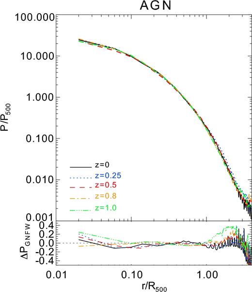
Top panel: Redshift evolution of the mean pressure P/P500 radial profiles, out to 4R500, of our sample of massive clusters in the AGN simulations. Different colours are for the results obtained at z = 0, 0.25, 0.5, 0.8 and 1. Bottom panel: Relative difference between the mean profiles shown in the top panel at a given redshift and the corresponding best-fitting GNFW pressure profile.
The deviations shown in the bottom panel of Fig. 6 are partially contributed by the presence of nearby clusters, groups, substructures or a clumpy gas distribution. It is also likely that part of the deviation stems from possible dependencies (which have not been taken into account) on redshift or mass of the parameters describing the model. However, to analyse properly these additional dependencies, it is necessary to have a sample of objects within a larger range of masses and redshifts than the one considered here. Deviations from the GNFW model or additional dependencies of the associated parameters (see e.g. Battaglia et al. 2012b; Le Brun et al. 2015) would imply a departure from the assumed self-similar evolution (see also Ramos-Ceja et al. 2015).
4 GAS CLUMPING
The existence of small dense clumps and density fluctuations throughout the ICM can bias high the derivation of the gas density profile from X-ray surface-brightness observations and, as a consequence, the estimation of all the X-ray derived quantities, such as entropy, gas mass and pressure (e.g. Eckert et al. 2015). In a similar way, also the ICM pressure can deviate from a smooth distribution, affecting the thermal SZ effect signal and its scaling relations with cluster mass and the SZ power spectrum (e.g. Battaglia et al. 2015). The level of gas density or pressure inhomogeneity in the ICM is usually characterized by a clumpiness parameter (Mathiesen et al. 1999), which, however, is not a directly observable quantity. In this respect, numerical simulations are useful instruments to quantify the degree of expected clumpiness, and to investigate its origin and its impacts on observational measurements (e.g. Nagai & Lau 2011; Roncarelli et al. 2013; Vazza et al. 2013; Zhuravleva et al. 2013; Battaglia et al. 2015).
4.1 Definitions
In the computation of the gas and pressure clumping factors we only take into account the X-ray emitting SPH particles, i.e. those particles with T ≥ 106 K. This temperature cut does not significantly affect the pressure clumping factor obtained from any of our simulations (see also Battaglia et al. 2015).

Median radial profiles of the SPH volume bias, as defined by equation (6), out to 2Rvir for the sample of 5 central groups (left-hand panel) and 24 central clusters (right-hand panel) within our three sets of simulations. Lines in black, blue and red stand for the results at z = 0 for the NR, CSF and AGN simulations, respectively, whereas the same line types connected by small dots stand for the results obtained at z = 1. Vertical lines in both panels represent the mean values of R500 and R200 for the AGN simulations.
Independently of the inclusion of this correction, as we will see throughout this section, our results on clumping are in broad agreement with the findings of previous studies performed with either SPH or Eulerian-based simulations including different sets of physical processes (e.g. Nagai & Lau 2011; Roncarelli et al. 2013; Vazza et al. 2013; Battaglia et al. 2015; Eckert et al. 2015).
4.2 Results on clumping
Fig. 8 shows the radial distribution of Cρ and CP obtained for the sample of 5 central groups and 24 central clusters within our three sets of simulations at z = 0. At the mass scale of groups, the gas density clumping factor shows values smaller than ∼2 within R200. Generically, the two radiative simulations produce similar results, with systematically lower degree of clumping than in the NR case. In fact, radiative cooling has the effect of removing high density, relatively cold gas from the hot phase, thus suppressing gas clumping. At the same time, feedback from SN driven winds and, even more, from AGN displace gas from high-density regions, thus further contributing to smooth the density and thermal distributions of the ICM (see e.g. Planelles et al. 2014; Rasia et al. 2014). As a consequence, there is a reduction in the number of small cold density clumps that are more prominent in outer cluster regions. These dense clumps are mainly associated with substructures being accreted to the centre of more massive central systems. This is the reason why the clumpiness is more important in outer regions, which are dynamically younger and still under the effects of ongoing matter accretion, than in inner regions. The density clumping factor shows a similar behaviour in clusters and in groups within R200. However, beyond this radius, Cρ in clusters is higher and steeper than in smaller systems. This is due to the fact that massive systems are more prone to significant merging and matter accretion since they are, on average, formed more recently.
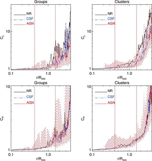
Left column: Top and bottom panels show, respectively, the median radial distribution at z = 0 of the gas density and pressure clumping factors, that is, Cρ and CP for the sample of groups within our simulations. Black, blue and red lines stand for the results obtained for the NR, CSF and AGN simulations, respectively. The coloured area in red stand for 1σ dispersion around the median profile of the AGN run. Vertical lines represent the mean values of R2500 and R200 in units of R500 for the sample of considered objects within the AGN simulations. Right column: Same results shown in the left column but for the sample of massive galaxy clusters.
Measurements of density clumping are quite uncertain. Indeed, only the application of indirect methods has led recently to some estimations. Simionescu et al. (2011) analysed Suzaku observations of the outskirts of the Perseus cluster. They measured values of gas fraction in the outer regions well in excess of the cosmic value, a result that they interpreted as spuriously induced by gas density clumping, with a clumping factor of Cρ ∼ 1–3 at R500 and Cρ ∼ 9–12 at 1.5 × R500. Walker et al. (2012) also obtained relatively large values for the clumping, with Cρ ∼ 1–3 at R500 and Cρ ∼ 2–9 at 1.5 × R500 for the PKS0745−191 cluster (cf. also Morandi, Nagai & Cui 2013). On the contrary, Eckert et al. (2013) used the deviations from self-similarity of the observed entropy profiles for a sample of 18 clusters for which both ROSAT measurements of X-ray surface brightness and Planck measurements of the SZ signal are available beyond R500. From their analysis, Eckert et al. (2013) inferred values of clumping Cρ ∼ 1.2 at R200, thus considerably lower than found by Simionescu et al. (2011). In a further analysis, Eckert et al. (2015) used a slightly larger sample of clusters observed with ROSAT and Planck together with a new technique to obtain unbiased density profiles from X-ray data. Their newly derived values, |$\sqrt{C_{\rho }}< 1.1$| for r < R500, are thus in good agreement with their previous measurements implying a modest gas density clumping.
It is with this large statistical sample that we compare our simulations in Fig. 9. Since the dispersion around the median clumping profiles is significant for our three models, we should take these results with caution. However, by looking at the median clumping profiles obtained for each set of simulations, there is a clear trend: both radiative simulations are in remarkably good agreement with the data whereas the NR runs produce systematically larger values ( ≳ 20 per cent beyond R200) than observed (see also Vazza et al. 2013). In general, results on density clumping from our radiative simulations favour small values of gas clumping, independently of the feedback scheme included. Thus, they are at variance with the large clumping factors found by Simionescu et al. (2011) from Suzaku observations.
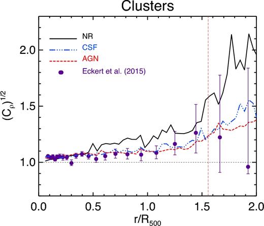
Comparison of the 3D median radial distribution at z = 0 of the gas density clumping factor for the sample of massive clusters within our simulations and the observations by Eckert et al. (2015). Black, blue and red lines stand for the results obtained for the NR, CSF and AGN simulations, respectively, whereas filled dots represent the observational data. The vertical dashed line represents the mean value of R200 in units of R500 for the sample of considered objects within the AGN simulations.
The bottom panels of Fig. 8 show that the pressure clumping behaves similarly to Cρ, with the exception that the radial behaviour of CP does not depend significantly on the physical model. This suggests that the small cold density clumps that enlarge the density clumping in outer regions of clusters and groups within our NR simulations are in pressure equilibrium with the surrounding medium and, thus, give a negligible contribution to the pressure clumping (see also Battaglia et al. 2015). In addition, although CP is slightly larger than Cρ within R200, it shows lower values outside this region.
Given the obvious connection between clumpiness and environment, it is interesting to analyse how it relates to the thermal or dynamical state of each cluster. To this purpose, we now analyse the distribution of clumpiness in the AGN simulations when clusters are divided in CC/NCC and in regular/disturbed objects (see Section 2.2). For each of these subsamples, we have computed the radial distributions of gas density and pressure clumpiness, that is, |$C_{\rho _{{\rm sub}}}$| and |$C_{P_{{\rm sub}}}$|. We compare these median profiles to the corresponding global median profile shown in Fig. 8. Fig. 10 shows the relative difference between the median profiles in gas density clumpiness (left-hand panels), |$\Delta C_{\rho }=(C_{\rho _{{\rm sub}}}- C_{\rho })/C_{\rho }$|, and pressure clumpiness (right-hand panels), |$\Delta C_P=(C_{P_{{\rm sub}}}-C_P)/ C_P$|, for the sample of CC/NCC (upper plots) and regular/disturbed systems (lower plots). As for the gas density clumpiness, when our sample is divided into CC and NCC-like clusters, there is no much difference between these two populations, showing the larger differences at r ≥ R200. Moreover, the two subsamples show negligible differences in clumpiness throughout the whole radial range, indicating that the radial distribution of Cρ in both cases is quite similar to the distribution of clumpiness obtained for the whole sample of clusters. Only at r ≥ R200, ΔCρ slightly deviates from zero, especially for the CC systems. On the contrary, if we analyse the radial distribution of ΔCρ obtained for the populations of regular and disturbed clusters, there is a clear difference between them. In particular, while regular objects show ΔCρ ∼ 0 out to ∼R200, disturbed clusters show a larger deviation already from ∼0.2R500. Whereas regular systems always tend to produce ΔCρ ≤ 0, disturbed clusters tend to show larger values of clumpiness and a larger cluster-to-cluster scatter than the global sample. A similar behaviour is obtained for ΔCP. In this case, however, both CC and NCC systems show ΔCP ∼ 0 at least out to ∼3R500, whereas the deviation between regular and disturbed clusters is already evident from ∼0.3R500.
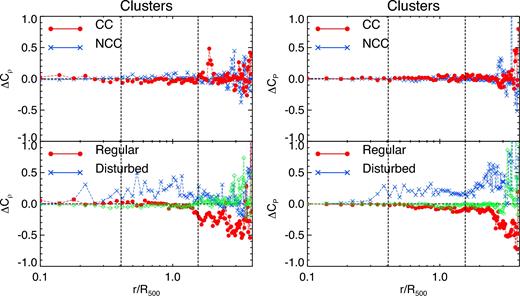
Left panel: Relative deviation, ΔCρ, between the median profile of gas density clumping obtained for the subsamples of CC/NCC and regular/disturbed clusters (top and bottom panels, respectively) in the AGN simulation with respect to the corresponding global median profile shown in Fig. 8. Profiles for CC and relaxed systems are represented in red by filled circles, whereas NCC or disturbed clusters are given by blue lines with crosses. Green lines in the bottom panel stand for the sample of clusters classified as in an intermediate state. Right panel: The same as in the left-hand panel but for the corresponding deviation in pressure clumping, ΔCP. Vertical lines indicate the mean values of R2500 and R200 for the sample of considered clusters.
These results indicate that, whereas density and pressure clumpiness is quite insensitive to the thermal properties of clusters in their core regions, it depends significantly on their global dynamical state. As shown in Biffi et al. (2016), this trend is also consistent with the HE deviation obtained for the same sample of clusters. In general, dynamically disturbed objects are still being formed and therefore their ICM is more inhomogeneous than in dynamically relaxed systems. Indeed, in previous studies the degree of ICM density clumping has been used as a criterion to distinguish between relaxed and unrelaxed systems (see Roncarelli et al. 2013). In this regard, Battaglia et al. (2015) also found a similar dependence on the dynamical state of their clusters, with relaxed systems showing the lower clumping values.
Fig. 11 shows that the density clumping factor generally increases with redshift, especially at r ≥ 2 × R500. This increase, which is slightly larger for our sample of groups, amounts to a factor of ∼4 at z = 0.8. A similar trend is also obtained for CP(r) for both groups and clusters. Given the relatively low number of systems and the large scatter of the profiles, our results have to be taken with caution. Nevertheless, a more pronounced clumping at high redshift, both in density and pressure, is in line with the younger age of systems at earlier epochs, when accretion from substructures and filaments is more efficient (see also Battaglia et al. 2015). A stronger increase of clumping for groups is consistent with the expectation that ram-pressure stripping is less efficient there than in clusters, thus causing a less efficient removal of gas from merging clumps.
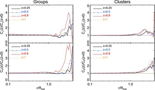
Left column: Top and bottom panels show, respectively, the ratio between the radial distribution of the gas density and pressure clumping factors at different redshifts, and the corresponding values at z = 0 for the sample of groups within our AGN simulations. Different line types stand for the ratios obtained at z = 0.25, 0.5, 0.8 and 1. Right column: The same as in the left column but for the sample of massive galaxy clusters.
Therefore, as predicted by simulations and confirmed by recent observational determinations, there is a certain level of clumpiness in the ICM that should be considered for precise X-ray and SZ measurements. In our simulations its degree is considerably lower than some values advanced to explain Suzaku observations and it is still consistent with other X-ray and SZ measurements of a local sample of clusters. However, caution in interpreting projected quantities should be applied as the clumpiness grows very rapidly outside the virial radius.
5 SZ SCALING RELATIONS
After analysing the pressure profiles and the gas clumping in our simulations, we consider now how these results translate in the SZ scaling relations. As anticipated in Section 2.2, to increase the statistics and to enlarge the mass range, here we will utilize the complete sample of simulated groups and clusters.
5.1 Definitions
We evaluated YSZ from Compton-y 2D maps obtained with a map making utility for idealized observations detailedly described in Dolag et al. (2005). The Comptonization parameter maps were computed using all gas particles in a cuboid of 5R500 × 5R500 × 10R500 (the last dimension is along the line of sight). Each projection was centred on the cluster centre, namely the location of the particle with the minimum gravitational potential as in the previous analysis. We calculate projected Compton-y maps along the three main axes for each cluster at redshift 0, 0.25, 0.5, 0.8 and 1. YSZ,500 and YSZ,2500 were calculated from 2D maps by integrating the Compton-y in circles with radii R500 and R2500.
5.2 The YSZ–M scaling relation
In the last decade a number of analyses of SZ observational data have been carried out to determine the scaling relation between the SZ signal and the total mass of clusters (see e.g. Giodini et al. 2013, for a review). The main outcomes of these analyses are that the SZ effect correlates strongly with mass and that the evolution of the YSZ–M relation agrees with the prediction from self-similarity. The intrinsic scatter is found to vary between 12 per cent (Hoekstra et al. 2012) and 20 per cent (Marrone et al. 2012), when cluster lensing masses are used, while in the combined SZ/X-ray study by Bonamente et al. (2008) the scatter is even lower, ∼10 per cent, when evaluated for masses obtained from HE. Recently, Czakon et al. (2015), using the Bolocam X-ray-SZ sample, reported a ∼25 per cent scatter and a discrepancy with the self-similar prediction that appears to be caused by a different calibration of the X-ray mass proxy with respect to other analyses. The larger scatter reported by Marrone et al. (2012) was explained as partially due to cluster morphology, while most of the segregation is caused by modelling clusters as spherical objects. Instead, in a previous work on a smaller set of 14 clusters, Marrone et al. (2009) found no clear evidence of morphological difference with respect to cluster dynamical state (classified as disturbed/undisturbed based on the X-ray-SZ peak offset). Simulations also tend to support the self-similar description for the YSZ–M relation, especially on cluster scales, where several studies (e.g. da Silva et al. 2004; Nagai 2006; Battaglia et al. 2012a; Kay et al. 2012; Sembolini et al. 2013; Pike et al. 2014; Gupta et al. 2016; Hahn et al. 2017) have found the relation to be robust when non-gravitational physics is included. However, with respect to observations, simulations predict a lower intrinsic scatter with a value that spans from 10 per cent (Nagai 2006) to less than 5 per cent (Sembolini et al. 2013). When doing this comparison, it is worth keeping in mind that simulation results are based on true masses, whereas observational scaling relations are computed either through X-ray or gravitational lensing.
In the left-hand panel of Fig. 12, we compare the YSZ,500–M500 relation obtained for our simulated cluster set with observations from Marrone et al. (2012) and the Cosmo sample from Planck Collaboration XX (2014a). The best-fitting relations obtained in the NR, CSF and AGN simulations are shown with different line types. In Table 2, we report the best-fitting values for normalization, power-law index and scatter obtained in each case. For the sake of clarity, we only show the data points for the AGN simulation (red asterisks). We note that the best-fitting relations obtained for our different models are close to each other over all the mass range sampled by our simulations. This is in agreement with the mean weighted pressure profiles shown in Fig. 2, which also demonstrates that the main contribution to the SZ signal comes from radii around R500, consistently with Kay et al. (2012), Sembolini et al. (2013) and Pike et al. (2014).
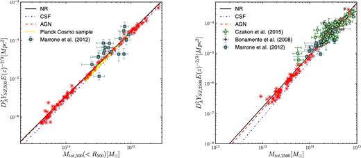
Relation between SZ flux and cluster mass within R500 (left-hand panel) and R2500 (right-hand panel) for the sample of simulated clusters. SZ results from simulations refer to the cylindrical Y. We plot the best-fitting relation obtained for the NR (black continuous line), CSF (blue dot–dashed line) and AGN (red dashed line) simulations. For the sake of clarity, only data for the AGN run is plotted (red asterisks). Different observational samples are used for comparison. In both panels, results from the analysis by Marrone et al. (2012) from LoCuSS–SZA clusters are shown as light-blue squares with error bars. In the left-hand panel, we also compare our simulations with the best-fitting relation obtained for the Planck Cosmo sample (yellow shaded area; Planck Collaboration XX 2014a). In the right-hand panel, we show the Chandra-BIMA/OVRO cluster sample by Bonamente et al. (2008) (stars with error bars) and the Bolocam X-ray-SZ sample BOXSZ by Czakon et al. (2015) (green dots with error bars).
Best-fitting parameters for the normalization, A, the slope, B and the scatter, |$\sigma _{{\rm log}_{10}}$| (as introduced in equations (11) and 12), describing the relation between YSZ and cluster mass evaluated within R500 and R2500. The pivot X0 is equal to 5 × 10¹⁴ and 2 × 10¹⁴ M⊙ (for R500 and R2500, respectively). The parameters are obtained for the complete sample of clusters and groups within the NR, CSF and AGN simulations. For completeness, we also show the best-fitting parameters obtained for the subsamples of regular/disturbed and CC/NCC systems in the AGN case.
| Simulation | Sample | A500 | B500 | |$\sigma _{log_{10} Y_{500}}$| | A2500 | B2500 | |$\sigma _{{\rm log}_{10} Y_{2500}}$| |
|---|---|---|---|---|---|---|---|
| NR | Complete | −4.282 ± 0.008 | 1.688 ± 0.012 | 0.062 | −4.542 ± 0.012 | 1.726 ± 0.017 | 0.085 |
| CSF | Complete | −4.382 ± 0.008 | 1.726 ± 0.011 | 0.062 | −4.712 ± 0.013 | 1.851 ± 0.019 | 0.098 |
| AGN | Complete | −4.305 ± 0.009 | 1.685 ± 0.013 | 0.067 | −4.585 ± 0.014 | 1.755 ± 0.020 | 0.104 |
| Reduced-CC | −4.253 ± 0.028 | 1.561 ± 0.071 | 0.047 | −4.584 ± 0.052 | 1.747 ± 0.144 | 0.081 | |
| Reduced-NCC | −4.291 ± 0.015 | 1.618 ± 0.037 | 0.055 | −4.548 ± 0.020 | 1.706 ± 0.059 | 0.082 | |
| Reduced-regular | −4.316 ± 0.013 | 1.639 ± 0.025 | 0.032 | −4.595 ± 0.030 | 1.745 ± 0.062 | 0.074 | |
| Reduced-disturbed | −4.249 ± 0.038 | 1.518 ± 0.105 | 0.073 | −4.485 ± 0.031 | 1.681 ± 0.107 | 0.076 |
In the same figure, we note some differences in the relation obtained from simulated data and observations. In particular, the 18 clusters observed by Marrone et al. (2012) in the redshift range around z ∼ 0.2 are plotted as grey squares with error bars. These results are based on weak-lensing cluster masses obtained from observations with the Subaru Telescope and on YSZ computed from observations with the SZ array (SZA). The simulations agree quite well with the data in normalization and slope but not in the scatter which is of the order of 20 per cent for Marrone et al. (2012) and 4–5 per cent in our simulated sample (see Table 2).
In Fig. 12, we also compare simulation results with those from the Planck Cosmo sample as presented in Planck Collaboration XX (2014a). This sample includes 71 clusters from different studies: the Early SZ cluster sample observed by Planck (Planck Collaboration XI 2011b), a smaller set of LoCuSS clusters (Planck Collaboration III 2013a) and a sample of XMM–Newton clusters (Planck Collaboration IV 2013b) observed by Planck. The reported best-fitting relation (in yellow) was obtained by applying the correction for the Malmquist bias. Observations report an intrinsic orthogonal scatter σlog Y at fixed mass of 6.3 per cent, thus similar to our best-fitting scatter reported in Table 2. However, Planck data show a slope, B = 1.79, which is steeper than the typical values found in our simulations, B = 1.68–1.73.
In the right-hand panel of Fig. 12, we report the same relation but for Δ = 2500, i.e. YSZ,2500–M2500. In this case, we compare results from our simulations with three different observational samples: the previously mentioned LoCuSS/SZA cluster sample by Marrone et al. (2012) (light-blue squares with error bars), the Chandra-BIMA/OVRO cluster sample analysed by Bonamente et al. (2008, grey stars with error bars) and the results regarding the BOXSZ sample reported by Czakon et al. (2015, green dots with error bars). The latter sample is composed by 45 galaxy clusters with a median redshift of 〈z〉 ∼ 0.42, that were observed with Bolocam and for which Chandra data were used. Czakon et al. (2015) report a 5σ shallower slope for their YSZ,2500–M2500 relation than is predicted by the self-similar model. A similar discrepancy was also recently found by Romero et al. (2016), who used a smaller set of clusters observed with MUSTANG and Bolocam.
Within these inner cluster regions, we see a distinction between models, with a lower normalization in the case of CSF clusters that is particularly visible when looking at systems with M2500 < 1014 M⊙. This trend is in qualitative agreement with what obtained in the pressure profiles weighted by radius (right-hand panel of Fig. 2), where AGN and CSF central groups show slightly lower pressure values (this effect is stronger when we consider the whole sample of groups and not only the isolated ones). The result on pressure profiles translates into a lower integrated cylindrical YSZ for galaxy groups. For clusters with larger masses (M2500 > 3 × 10¹⁴ M⊙) the difference is not so pronounced, and even reduced by almost a half in the CSF case. However, we would like to stress again that the SZ properties we present here refer to the ‘complete’ sample, while the results presented in Fig. 2 are for the reduced sample of systems.
Here again we note some discrepancy between the observational data sets. The analysis by Czakon et al. (2015) on BOXSZ data covers the highest mass range and reports a shallow slope (B2500 = 1.06 ± 0.12) and a 25 per cent scatter in data. As for the analysis by Bonamente et al. (2008) data show a large scatter and the best-fitting relation (A2500 = −3.83, B2500 = 1.66 ± 0.20) has a slightly higher normalization and a shallower slope. Marrone et al. (2012) instead obtain a slope and normalization (A2500 = −4.56, B2500 = 1.81) in close agreement with our results. It is worth pointing out that masses in the analysis by Czakon et al. (2015) do rely on the Mgas proxy, those from Bonamente et al. (2008) are based on X-ray analysis and assumption of HE, while Marrone et al. (2012) use masses derived from weak lensing analyses. Since we use true masses in our analysis, we expect better agreement with Marrone et al. (2012) given that, in principle, weak lensing measurements provide mass estimates closer to true cluster masses, provided that systematics are sufficiently under control (e.g. Meneghetti et al. 2010; Becker & Kravtsov 2011; Rasia et al. 2012; Mantz et al. 2016). Czakon et al. (2015) report instead that most of the discrepancy with respect to the self-similar scaling is caused by differences in the calibration of the X-ray mass proxies adopted in different analyses of observational data. The tension of simulations with the results by Bonamente et al. (2008) could be alleviated by accounting for the effect of hydrostatic bias, which causes X-ray masses to be underestimated by 10–20 per cent (e.g. Rasia et al. 2012, and references therein). Accounting for a possible hydrostatic bias in a self-consistent way would clearly require that also the value of the characteristic radii, R500 and R2500, should be decreased accordingly. A proper inclusion of the effects of hydrostatic bias on the scaling relations is beyond the scope of this paper and we refer the reader to specific analyses devoted to it (e.g. Biffi et al. 2016, and references therein).
In our simulations the core thermal properties or the cluster dynamical state affect the scatter in the YSZ–M relations. Table 2 reports the best-fitting values obtained for the power-law relation of equation (11) when the relevant quantities are computed within R500 and R2500. In particular, we show results for the complete set of groups and clusters in our three models and for the two distinct subsamples of regular/disturbed and CC/NCC clusters in our AGN simulations.
As discussed previously, when we consider the complete sample of systems we obtain, for all models, a scatter of 6–7 per cent at R500 and 8–10 per cent at R2500, with the AGN model showing the largest scatter. If we analyse instead the results obtained for the subsamples of regular/disturbed and CC/NCC clusters in our AGN simulations we get interesting conclusions. At R500, we note that cluster dynamical state has a minor impact on normalization and slope of the scaling relations. As for the scatter, it is higher (≃7 per cent) for the dynamically disturbed clusters, whereas it clearly decreases for relaxed systems (≃3 per cent). However, in the case of CC and NCC systems we see that the scatter at R500 is similar, with values of ≃5 and 5.5 per cent, respectively.
As for the results at R2500 the CSF model has a higher slope and normalization with respect to the other two. At the scale of clusters with 1014 M⊙ < M2500 < 1015 M⊙, corresponding to the range of the observational samples of Bonamente et al. (2008), Czakon et al. (2015) and Marrone et al. (2012), the difference among models is reduced by a factor of ∼2.5. Considering only the disturbed subsample gives a tilt to the relation, namely a slightly higher normalization than for the regular systems. At the same time, the scatter obtained for disturbed systems is close to that for relaxed clusters, with values around 7–8 per cent. In this case, NCC clusters also show a similar scatter as CC systems. This is consistent with the results on pressure profiles displayed in Fig. 3 for CC and NCC clusters, showing a similar scatter at radii below 0.1R500.
5.3 The evolution of the YSZ–M relation
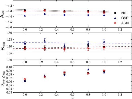
Redshift evolution of the YSZ,500–M500 scaling relation for the complete set of groups and clusters in the NR (black circles), AGN (red asterisks) and CSF (blue triangles) cases. In the three panels (from top down), we show the evolution of the normalization A500, the slope, B500 and the scatter, |$\sigma _{log_{10} Y_{500}}$|, of the relation. For the normalization and the slope we overplot, with dotted and dashed lines respectively, the best-fitting relation for redshift evolution. The self-similar value for the slope is represented in the middle panel with a black continuous line.
As shown in the top panel of Fig. 13, the normalization A500 remains almost constant with redshift. The radiative CSF simulation has the lowest normalization, in agreement with the results reported in the left-hand panel of Fig. 12 at z = 0. As shown in previous works (e.g. Fabjan et al. 2011; Planelles et al. 2014), the residual variation of cluster properties in radiative simulations with respect to NR ones is a consequence of overcooling that removes gas from the hot phase. At the same time, including AGN feedback partially prevents cooling and conversely brings NR and AGN normalizations to be closer. The middle panel of Fig. 13 reports the slope B500 for the three models: while in the NR and AGN case the slope is very close to the expected self-similar value (B500 = 5/3), the CSF simulation shows slightly steeper slopes at all redshifts with a small departure (less than ∼5 per cent) from self-similarity that is constant with increasing redshift. Since the slope does not differ significantly with physics, the differences in normalization are effective and do not depend upon the choice of the pivotal point. As for the scatter of the YSZ–M relation, previous findings from simulations (e.g. Sembolini et al. 2013) show that the scatter remains constant and at low levels. In our case, the scatter has values around 0.05–0.09 and increases with redshift, but if we focus only on massive clusters as in Sembolini et al. (2013), the scatter remains constant and at lower levels, ∼0.03–0.05. A small change in the best-fitting values for the normalization and slope parameters as the simulation model is changed was also noted by Kay et al. (2012) for their set of simulated clusters.
5.4 The effect of clumpiness and the YSZ–YX relation
In principle, X-ray measurements of gas mass and temperature can be used to predict the SZ effect signal. In particular, providing that clusters are isothermal, one can rewrite the integrated thermal pressure as |$Y_{{\rm SZ}} D^2_{\rm A} \propto T_{\rm e} \int n_{\rm e} {\rm d}V = M_{{\rm gas}} T_{\rm e}$|. This argument led Kravtsov et al. (2006) to introduce the X-ray analogue of the SZ Comptonization parameter, YX, defined as the product of the X-ray derived gas mass and temperature. In principle, in observations, the comparison between YSZ and YX can provide information both on the inner ICM thermal structure and on the clumpiness in gas density. In fact, X-ray and SZ signals have a dependence on gas density, ne, that is, respectively, quadratic and linear and therefore differences between the two signals arise in the presence of inhomogeneities in the gas distribution that would boost YX with respect to YSZ (e.g. Giodini et al. 2013). Furthermore, any inhomogeneity in the ICM thermal structure would induce a difference between the electron temperature, that enters in YSZ, and the spectroscopic temperature, which enters in YX (e.g. Rasia et al. 2014). We remind here that to compute YSZ from simulations we use the mass-weighted temperature profile (Tmw), while to obtain YX we employ the spectroscopic-like temperature (Tsl), as defined by Mazzotta et al. (2004), excising particles within 0.15R500.
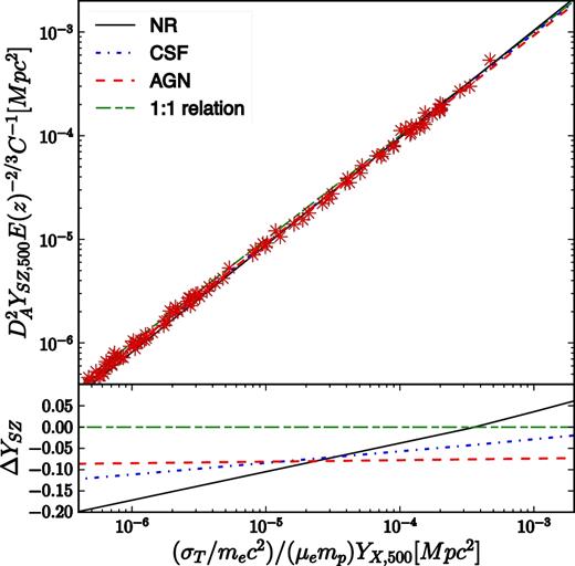
Upper panel: Relation between the spherically integrated SZ flux and YX at R500 for the complete sample of simulated systems. The SZ flux is obtained by multiplying the cylindrical YSZ with the parameter C (described in Section 5.4). Best-fitting relations are plotted with black continuous, blue dash–dotted and red dashed lines for the NR, CSF and AGN simulations. For the sake of clarity, data (red asterisks) are plotted only for the AGN case. YX is evaluated using core-excised (0.15–1R500) spectroscopic-like temperatures. The green long-short dashed line stands for the identity relation. Lower panel: Residuals of the YSZ–YX relation computed with respect to the identity relation, where ΔYSZ = (YSZ − YSZ,identity)/YSZ. Same legend as in upper panel applies.
As before, we compute the best-fitting relations following equation (11). For our simulated clusters we find that in the NR case clusters have the highest slope (B = 1.04, 1.01, 1.00 for NR, CSF and AGN, respectively), and both radiative models show the highest normalization (A = 0.12, 0.03, −0.02 for NR, CSF and AGN, respectively). Differences between the three models are of the order of at most ∼12 per cent, as we can see in the bottom panel of the same figure, where we show the residuals of our models with respect to the theoretical identity relation. In fact, we note that for our two radiative models the YSZ–YX relation is close to the identity relation (represented by the green long-short dashed line). In the case of the AGN model, we obtain a good agreement with the relation provided by Arnaud et al. (2010), that reports a value of YSPH/CYX = 0.924 ± 0.004 for the slope fixed to one. Our simulated clusters show a scatter of ∼0.03–0.04 in all models (for the sake of clarity we only plot data for the AGN case), being similar to what found from observational data (e.g. Arnaud et al. 2010).
Since we use the true gas mass obtained from simulations in the computation of both YX and YSZ, their comparison provides information on the deviation between Tsl, entering in the computation of YX, and Tmw, entering instead in YSZ (e.g. Biffi et al. 2014). In this case, keeping in mind that the innermost part of the cluster is excised when computing Tsl, there is only a slight deviation from the identity relation that is due to this temperature inhomogeneity. Radiative simulations generally show a smoother ICM thermal distribution than NR runs (e.g. Planelles et al. 2014). In principle, as found by Rasia et al. (2014), there should be a distinct behaviour in NR and radiative simulations that is a clear signature of two counteracting processes: the cooling process, that removes the low-entropy gas from the diffuse phase, and the heating by feedback processes, that prevents the gas removal. When both effects are at work, the temperature contrast between the clumps and the diffuse medium is lower. At the same time, this effect should be particularly relevant for clusters with larger masses, that are more affected by inhomogeneities from gas accretion. In our case, however, thanks to the improved description of mixing of the new hydro scheme, both radiative and NR runs are quite close to each other, thus indicating a more similar ICM thermal distribution in all cases.
As already mentioned, we compute YX using the true gas mass obtained from simulations, which however is not an observable. For an estimate of the effect that the bias in clumping has on the YSZ–YX relation we can use the data previously presented in Section 4. In the two upper panels of Fig. 8, we have shown that the median gas density clumping factor, Cρ, is of the order of 1–3 within R500 at the scale of the groups and clusters of the reduced sample. To obtain an estimate of how the YSZ–YX relation would change due to the clumping, we compute the mean Cρ inside R500 for clusters and groups separately. In this case, gas masses would increase by a factor |$\sqrt{\langle C_{\rho }\rangle }$|, which is equal to 1.051, 1.032, 1.032 for groups (〈M500〉 ∼ 1.9 × 10¹⁴h−1 M⊙) and to 1.124, 1.076, 1.076 for clusters (〈M500〉 ∼ 7.7 × 10¹⁴h−1 M⊙), respectively in the NR, CSF and AGN simulations. For radiative simulations the bias at the group scale would translate into a ∼3–4 per cent shift towards higher gas masses (or, equivalently, YX), compatible with the scatter of our data, while the shift would be two times larger (∼7.5 per cent) at the level of clusters. For the NR simulations the discrepancy would be, as expected, even larger (∼5 per cent and 12 per cent for groups and clusters, respectively). Due to the different behaviour at the group and cluster scales, the slope of the YSZ–YX relation we would obtain would be shallower, with an estimated value of B ∼ 0.85 for all the three different physics.
6 CONCLUSIONS
We have performed a detailed analysis of the ICM thermal pressure distribution of a sample of simulated galaxy clusters and groups, with the main purpose of analysing the existing connection between pressure profiles, ICM clumping and SZ scaling relations.
Our sample of groups and clusters has been extracted from a set of hydrodynamical simulations performed with a version of the GADGET-3 code that includes an improved description of SPH (Beck et al. 2016). We analysed three sets of simulations: besides a NR simulation set, we also considered two sets of radiative simulations, a first one including star formation and stellar feedback (CSF set), and a second one also including the effect of gas accretion on to SMBHs and the ensuing AGN feedback (AGN set). Based on different cluster properties, we have classified the systems in our AGN simulations in CC and NCC haloes (see Rasia et al. 2015, for further details) and, depending on their global dynamical state, in regular or disturbed systems (see also Biffi et al. 2016). These simulations, that we analysed out to z = 1, allow us to characterize in detail the ICM pressure distribution, the ICM clumping and the SZ scaling relations as a function of redshift, ICM physics, cluster mass and cluster dynamical state.
Our main findings can be summarized as follows:
Independently of the physics included in our simulations, the mean pressure profiles obtained for our sample of groups and clusters show a good agreement with different observational samples (e.g. Arnaud et al. 2010; Sun et al. 2011; Planck Collaboration V 2013c; Sayers et al. 2013; McDonald et al. 2014). In particular, in the case of clusters the agreement is within 1σ at r/R500 ≲ 1, while in outer regions (r ≳ R500) simulated profiles are systematically higher (by ∼20 per cent) than the universal profile presented in Arnaud et al. (2010). In the case of groups, our AGN simulations produce pressure profiles that agree within ∼15–20 per cent with the observations reported by Sun et al. (2011) and with the universal fit of Arnaud et al. (2010). This general consistency is also supported by a quantitative comparison between fitting parameters of the GNFW model.
When we analyse separately the pressure profiles of the samples of CC and NCC clusters in the AGN set, we also obtain a good agreement with observed profiles of these two cluster populations (e.g. Sayers et al. 2013; McDonald et al. 2014). Namely, whereas at intermediate and outer cluster radii pressure profiles of CC and NCC are similar (within a few per cent) to each other, they are clearly different in inner clusters regions, r ≤ 0.2R500, with CC clusters showing higher central pressure values (by a factor ∼2.5) and steeper profiles. As shown by Rasia et al. (2015), this sample of CC and NCC systems also shows a good agreement with observational data in terms of entropy and iron abundance profiles.
In agreement with observational data (e.g. McDonald et al. 2014; Adam et al. 2015), we obtain in all cases a redshift evolution of the pressure profiles of massive clusters that is consistent with the self-similar one, at least back to z = 1. The major discrepancies between simulated and observed profiles appear in very central and outer cluster regions, being in any case smaller than ∼10–15 per cent.
In accordance with previous numerical studies (e.g. Roncarelli et al. 2013; Battaglia et al. 2015), the gas density clumping derived in our simulations increases with the distance to the cluster centre. In addition, its magnitude also increases with increasing redshift, with the mass of the considered systems and in dynamically unrelaxed objects. A similar trend is also found for the gas pressure clumping, which shows, however, a lower magnitude.
While our NR simulations produce quite higher values of the gas density clumping ( ≳ 20 per cent beyond R200), both of our radiative runs produce lower values (|$\sqrt{C}_{\rho }\sim 1.2$| at R200). While this level of clumping is in good match with, for instance, the observational estimate by Eckert et al. (2015), it is significantly smaller than that inferred to explain reported measurements of high entropy in the outskirts of clusters (e.g. Simionescu et al. 2011).
The YSZ–M scaling relation of our simulations is in good agreement with observational data at the scale of massive clusters (e.g. Bonamente et al. 2008; Marrone et al. 2012; Czakon et al. 2015). In addition, consistently with previous numerical analyses (e.g. Kay et al. 2012; Sembolini et al. 2013; Pike et al. 2014), our results at R500 do not show any significant dependence on the physics included. Moreover, for all our models, normalization and slope of the relation do not show any clear redshift evolution, but only an increase in scatter (from 6 to 9 per cent for z = 0–1).
As for the scatter in the YSZ–M relations, we predict a clear dependence on the cluster dynamical state, with disturbed clusters showing ∼2 times larger scatter than regular systems at R500. This finding is not reflected in the CC/NCC samples confirming that the cluster dynamical state, measured at larger scales, is not strongly correlated with its cool-coreness (Meneghetti et al. 2014; Donahue et al. 2016).
While observations and simulations agree in that galaxy clusters behave as a homogeneous population of objects at intermediate radii, 0.15R500 < r < R500, cluster core regions and cluster outskirts are quite sensitive to a number of dynamical and feedback processes. Given their definitions, X-ray and SZ observations provide a complementary description of the ICM thermodynamics, with the former being better suited to prove inner high-density cluster regions, while the latter being more sensitive to outer low-density regions. From an observational point of view, however, constraining the outskirts of clusters is challenging because they require observations with high sensitivity: long exposures to detect low surface brightness and sharp point spread functions to remove contributions from point-like sources (e.g. Reiprich et al. 2013, for a recent review). In particular, although ICM clumping can affect derived X-rays and SZ cluster properties, current estimations are still uncertain. A detailed analysis of cluster outskirts will require the next generation of high-sensitivity X-ray observatories, such as athena2 (e.g. Pointecouteau et al. 2013; Nandra et al. 2013; Ettori et al. 2013b), in combination with high-resolution SZ observations. Simulations, like those presented in this paper, will represent an ideal interpretative framework to unveil the physical processes determining the structure of the ICM pressure, also in view of an improved calibration of galaxy clusters as precise tools for cosmology.
Acknowledgments
The authors would like to thank Volker Springel for allowing us to access the developer version of the GADGET code and Matteo Costanzi for helping us in the use of the MCMC algorithm. We also would like to thank Mauro Roncarelli, Daisuke Nagai, Dominique Eckert, Jack Sayers and Michael McDonald for useful comments and discussions as well as the anonymous referee for constructive comments that helped to improve the presentation of our results.
We acknowledge financial support from PIIF-GA 2013-627474, NSF AST-1210973, PRIN-MIUR 201278X4FL, PRIN-INAF 2012 ‘The Universe in a Box: Multi-scale Simulations of Cosmic Structures’, the INFN INDARK grant, ‘Consorzio per la Fisica’ of Trieste, CONICET-Argentina, FonCyT. SP also acknowledges support by the Spanish Ministerio de Economía y Competitividad (MINECO, grants AYA2013-48226-C3-2-P and AYA2016-77237-C3-3-P) and the Generalitat Valenciana (grant GVACOMP2015-227). DF acknowledges financial support from the Slovenian Research Agency (research core funding No. P1-0188). CRF acknowledges funding from CONICET, FonCyT and SeCyT-UNC, Argentina. AMB is supported by the DFG cluster of excellence ‘Universe’ and by the DFG Research Unit 1254 ‘Magnetization of interstellar and intergalactic media’ and by the Leibniz-Rechenzentrum via project ‘pr92ju’. MG is supported by NASA through Einstein Postdoctoral Fellowship Award Number PF-160137 issued by the Chandra X-ray Observatory Center, which is operated by the SAO for and on behalf of NASA under contract NAS8-03060. Simulations are carried out using Flux HCP Cluster at the University of Michigan, Galileo at CINECA (Italy), with CPU time assigned through ISCRA proposals and an agreement with the University of Trieste, and PICO at CINECA through our ISCRA project IscrC_GALPP2.
REFERENCES
