


Abstract
We perform a measurement of the mass–richness relation of the redMaPPer galaxy cluster catalogue using weak lensing data from the Sloan Digital Sky Survey (SDSS). We have carefully characterized a broad range of systematic uncertainties, including shear calibration errors, photo-z biases, dilution by member galaxies, source obscuration, magnification bias, incorrect assumptions about cluster mass profiles, cluster centring, halo triaxiality and projection effects. We also compare measurements of the lensing signal from two independently produced shear and photometric redshift catalogues to characterize systematic errors in the lensing signal itself. Using a sample of 5570 clusters from 0.1 ≤ z ≤ 0.33, the normalization of our power-law mass versus λ relation is log10[M200m/h−1 M⊙] = 14.344 ± 0.021 (statistical) ±0.023 (systematic) at a richness λ = 40, a 7 per cent calibration uncertainty, with a power-law index of |$1.33^{+0.09}_{-0.10}$| (1σ). The detailed systematics characterization in this work renders it the definitive weak lensing mass calibration for SDSS redMaPPer clusters at this time.
1 INTRODUCTION
The abundance of galaxy clusters is a powerful cosmological probe (Albrecht et al. 2006). In this work, we measure the relationship between the weak lensing masses and the optical richness of galaxy clusters. Weak lensing offers a unique key to understanding the masses of structures in the Universe, due to its equal sensitivity to dark and baryonic matter (Schneider 2006). Galaxy clusters are a good target for weak lensing due to their high masses and thus large lensing distortions. Using weak lensing mass measurements, we can better understand the relationship between cluster masses and other observables, which aids scientific goals such as measurements of cluster abundances for cosmology.
Weak lensing exploits the deflection of light rays and the resulting distortion of galaxy shapes by gravitational fields. By measuring statistical changes in the shapes of more distant galaxies, we can detect the gravitational fields sourced by intervening matter and therefore probe the distribution and amount of matter in the Universe (Schneider 2006). Weak lensing has been commonly used to characterize the matter in galaxies (e.g. Brainerd, Blandford & Smail 1996), groups (e.g. Leauthaud et al. 2010) and galaxy clusters (e.g. Sheldon et al. 2004; Johnston et al. 2007b; von der Linden et al. 2014; Hoekstra et al. 2015; Okabe & Smith 2016; van Uitert et al. 2016), as well as the large-scale distribution of matter through the technique known as cosmic shear (e.g. Bacon, Refregier & Ellis 2000; Kilbinger et al. 2013; Becker et al. 2016).
Galaxy clusters, the target of this weak lensing study, represent the most massive gravitationally bound structures in the Universe (e.g. Allen, Evrard & Mantz 2011). They consist of multiple galaxies in a large dark matter halo, usually with one large elliptical galaxy in the centre. These galaxies are systematically different from other elliptical galaxies (e.g. von der Linden et al. 2007). The dominant baryonic component is a reservoir of a hot gas held by the potential well of the dark matter halo, but this gas is visible only in the X-ray (thermal bremsstrahlung) and radio [through scattering of photons from the cosmic microwave background (CMB)]. All these properties can be used to construct cluster catalogues, based on characteristics such as distortions of the observed spectrum of CMB photons along the line of sight to the clusters (Bleem et al. 2015), extended X-ray emission (Piccinotti et al. 1982) or simply an overdensity of optically detected galaxies at the same redshift. In this paper, we use the redMaPPer optical cluster finder (Rykoff et al. 2014, henceforth RM I), described in Section 3.1. Cluster catalogues typically have a ranking mechanism based on a mass proxy such as X-ray luminosity or the number of galaxies in the cluster. We calibrate the relationship between the redMaPPer mass proxy, the summed galaxy membership probability λ (also known as the optical richness) and the masses derived from weak lensing measurements.
Previous work on the redMaPPer catalogue mass–richness relation has included comparison to other cluster data sets and weak lensing measurements from several different imaging surveys (Rozo & Rykoff 2014; Du et al. 2015; Saro et al. 2015; Miyatake et al. 2016). Because of widely varying parametrization choices, we will discuss these results further in Section 7, including conversions necessary to compare amongst them and against our work. The work presented here is the largest sample for which such measurements have been made; we obtain high signal-to-noise ratio measurements of the lensing signal in several richness bins and two redshift bins, and also use what we believe to be the most complete model for the lensing signal and its systematics. Our results are consistent with previous measurements, but precisely calibrate the systematic uncertainty associated with the weak lensing masses.
We discuss the background of our weak lensing procedure in Section 2. We then discuss the redMaPPer algorithm and its application to Sloan Digital Sky Survey (SDSS) Data Release 8 (DR8) data, particularly its richness estimator λ, in Section 3.1. The lensing shear catalogue is described in Section 3.2. The mass model that we use is detailed in Section 4, and we address a variety of sources of systematic error in Section 5. Our results from model fits are given in Section 6. We summarize and conclude in Section 7. Throughout the paper, except where noted, we assume a flat Λ cold dark matter (ΛCDM) cosmological model with Ωm = 0.3, σ8=0.8 and h100 = 1. Unless otherwise specified, all distances are physical distances (rather than comoving).
2 WEAK LENSING BACKGROUND
The deflection of light by gravity affects the apparent shape, size and number density of galaxies. These effects can be used to measure the relationship between dark matter and visible matter, or more generally to probe cosmological models (Bartelmann & Schneider 2001; Hu 2002; Huterer 2002; Abazajian & Dodelson 2003; Refregier 2003; Schneider 2006; Hoekstra & Jain 2008; Massey, Kitching & Richard 2010). An overdensity of matter, such as a galaxy or galaxy cluster, will cause a slight tangential alignment of galaxies at more distant redshifts; an underdensity, such as a void, will cause a slight radial alignment. In addition, the number density (e.g. Broadhurst, Taylor & Peacock 1995) or distribution of quantities such as redshift (e.g. Coupon, Broadhurst & Umetsu 2013) and size (e.g. Schmidt et al. 2009) will be altered, due to effects that shrink or enlarge the galaxy images on the sky. Shape distortion is usually called the lensing shear, while the other effects come under the umbrella of lensing magnification. Since weak lensing (as opposed to strong lensing) results in only slight differences in observed galaxy properties, it must be measured statistically.
To account for the survey mask, which otherwise might impose a small signal at large radii due to systematic errors that correlate with the survey boundaries, we subtract the ΔΣ estimate around random points from our real signal before the boost factor is applied (see e.g. Mandelbaum et al. 2005, 2013), also on a per-bin basis.
3 DATA
In this work, we use data from the SDSS (York et al. 2000; Eisenstein et al. 2011). Both our cluster and weak lensing catalogues derive from SDSS DR8 (Aihara et al. 2011).
3.1 The redMaPPer cluster catalogue
redMaPPer is a red-sequence photometric cluster finding algorithm (RM I), built around the optimized richness estimator developed in Rozo et al. (2009b) and Rykoff et al. (2012). Briefly, redMaPPer identifies galaxy clusters as overdensities of red galaxies, and estimates the probability that each red galaxy is a cluster member following a matched filter approach that models the galaxy distribution as the sum of a cluster and background component. The cluster richness λ is the sum total of the membership probabilities of all the galaxies. The cluster radius Rλ used for estimating the cluster richness is self-consistently computed with the cluster richness, ensuring that richer clusters have larger cluster radii. The radius Rλ is selected to maximize the signal-to-noise ratio of the richness measurements. The redMaPPer cluster richness λ has been shown to be tightly correlated with cluster mass by comparing λ to well-known mass proxies such as X-ray gas mass and Sunyaev–Zel'dovich (SZ) decrements. The original (v5.2) redMaPPer algorithm was published in RM I, to which the reader is referred for further details. Here, we utilize the v5.10 version of the algorithm, which introduced a variety of small improvements; we refer the reader to Rozo et al. (2015b, hereafter RM IV) for details.
The redMaPPer algorithm was applied to SDSS DR8 data (Aihara et al. 2011) in RM IV. The redMaPPer catalogue is restricted to the |${\sim } 10\,000\,\deg ^2$| of contiguous imaging used by the Baryon Oscillation Spectroscopic Survey (BOSS; Dawson et al. 2013). Roughly 2/3 of the survey falls in the Northern Galactic Cap, and 1/3 in the Southern Galactic Cap. The sky was imaged in five bands (ugriz), and we have imposed a limiting magnitude i < 21, which is a conservative estimate for the full footprint (see Rykoff, Rozo & Keisler 2015). redMaPPer utilizes the five-band imaging data to self-calibrate a model for red-sequence galaxies, and then applies this model to identify red galaxy overdensities and to estimate the corresponding photometric redshift of the galaxy clusters. SDSS redMaPPer photometric redshifts are accurate at the 0.005–0.01 level, depending on redshift. Here, we ignore the uncertainty associated with the cluster photometric errors. We have verified that randomly perturbing every cluster by its assigned photometric redshift uncertainty impacts our conclusions at less than the 1 per cent level, demonstrating that the cluster photo-z uncertainties are indeed negligible for this analysis.
The redMaPPer algorithm explicitly assumes that the centre of each cluster's halo coincides with the location of one of the brightest galaxies in the cluster, though not necessarily the brightest. Indeed, an important feature of redMaPPer is that it does not simply choose a cluster centre, it also attempts to estimate the probability pcen that each redMaPPer cluster is properly centred. The probability is estimated based on each galaxy's luminosity, photometric redshift and local galaxy density. redMaPPer relies on a Bayesian classification scheme with empirical, self-calibrated filters for the distribution of central and satellite galaxy properties, modified to take into account that every cluster contains one and only one central galaxy. For details, we refer the reader to RM I. Given the probability pcen for each cluster, the fraction of well-centred clusters over the entire cluster catalogue is simply |$P_{\rm cen}= N_{\rm clusters}^{-1}\sum p_{\rm cen}$|, where the sum is over all clusters in the catalogue. As discussed in Section 5.2, the fraction Pcen is an important systematic parameter in our analysis.
Cluster random points were generated using the updated method of Rykoff et al. (2016). In brief, we first sample a cluster from the redMaPPer cluster catalogue. This gives us the richness and redshift of our random point. We then randomly select a right ascension and declination within the survey footprint. If the survey is not sufficiently deep to have detected a cluster at that location, we reject the cluster, while keeping track of the number of times NR which each cluster is rejected. If the survey is sufficiently deep to detect our randomly selected cluster, then the cluster is added to the random catalogue at the randomly drawn position. The procedure is iterated until the random catalogue achieves the desired number of random points. Let N be the number of times that a particular cluster appears in the random catalogue, and N΄ by the number of times the cluster was rejected as a random point. We assign a weight w = (N + N΄)/N to each instance of this cluster in the random catalogue. This ensures that the weighted random catalogue exactly traces the richness and redshift distribution of the parent cluster catalogue.
To perform the weak lensing measurement, we bin the clusters in four richness bins and two redshift bins, for a total of eight bins. The bins are detailed in Table 1. We note that the largest bin has a very broad range of λ, but we checked alternate binning schemes and found no statistically significant differences between our final results. Our fiducial binning scheme has roughly equal signal-to-noise ratio for all richness and redshift bins.
Binning scheme for the redMaPPer clusters and characteristics of the clusters in each bin, including richness λ, redshift z and probability of correct centroid Pcen. The typical Nrand/N for the random catalogues is ∼22, and the typical mean richness and redshift are consistent for the random to ≲ 1 per cent. All averages are weighted by the same lensing weights we use to generate stacked models.
| λ range | Mean λ | z range | Mean z | Mean Pcen | No. of clusters |
|---|---|---|---|---|---|
| [20, 30) | 24.1 | [0.1, 0.2) | 0.153 | 0.87 | 767 |
| [20, 30) | 24.1 | [0.2, 0.33) | 0.260 | 0.87 | 2531 |
| [30, 40) | 34.4 | [0.1, 0.2) | 0.154 | 0.87 | 306 |
| [30, 40) | 34.5 | [0.2, 0.33) | 0.259 | 0.87 | 940 |
| [40, 55) | 46.3 | [0.1, 0.2) | 0.156 | 0.89 | 178 |
| [40, 55) | 46.5 | [0.2, 0.33) | 0.259 | 0.88 | 449 |
| [55, 140) | 73.2 | [0.1, 0.2) | 0.152 | 0.90 | 104 |
| [55, 140) | 71.8 | [0.2, 0.33) | 0.257 | 0.88 | 295 |
3.2 Lensing data
We use a shear catalogue first presented in Reyes et al. (2012), covering approximately 9000 deg2 and containing 39 million galaxies, or 1.2 galaxies arcmin−2. This catalogue derives from SDSS images as of DR8 (York et al. 2000; Aihara et al. 2011). The images were analysed with the re-Gaussianization algorithm1 (Hirata & Seljak 2003), which calculates adaptive second-order moments for the galaxy and point spread function (PSF) by fitting elliptical Gaussians to the images, and then combines these moments and a correction for low-order non-Gaussianity to produce a measured distortion e. We are interested in lensing shears, not distortions,2 so we must correct for the difference, and also for the fact that shears do not add linearly (Bernstein & Jarvis 2002). The average sensitivity of the mean distortion of the shape sample to an applied shear is usually called the responsivity, which for unweighted measurements is |$\mathcal {R} \approx 1-e_{\mathrm{rms}}^2$|. For this catalogue the appropriate value of erms is 0.365 (Reyes et al. 2012). We use the approximation here and not a full calculation of |$\mathcal {R}$|, but our value is consistent with the more detailed analysis. We also apply a multiplicative shear calibration factor of 1.02, as discussed in Mandelbaum et al. (2013). Further characterization of the systematic errors in this catalogue was carried out in Mandelbaum et al. (2012, 2013).
The photometric redshifts in this catalogue were calculated using the Zurich Extragalactic Bayesian Redshift Analyzer, or zebra (Feldmann et al. 2006). zebra is a template-fitting software; for this catalogue, four observed spectral energy distributions (SEDs) and two synthetic blue galaxy spectra from Benítez (2000) were used, along with 25 additional interpolated templates created between pairs of the six original templates. The performance of the photometric redshifts and their impact on weak lensing measurements was explored by Nakajima et al. (2012). The starburst-type galaxies, accounting for approximately 10 per cent of the original sample, were found to be unreliable based on comparison with a reference sample and were removed from the final catalogue. There is a remaining known bias for galaxies with z ≳ 0.4. We know the true dN/dz based on the work of Nakajima et al. (2012), so we can correct the effect of bias and scatter if we know the lens redshifts in the sample. This bias is worse as redshift increases; it is 3 per cent for the distribution of cluster redshifts in our lower redshift bin (z = 0.1–0.2) and 11 per cent for the distribution of cluster redshifts in our higher redshift bin (z = 0.2–0.33). All results shown in this paper have these corrections applied. The associated systematic uncertainty on ΔΣ is 2 per cent. The uncertainty in the amplitude of the ΔΣ profile due to the use of photometric redshifts was estimated by comparing the different lensing amplitudes for the source population as estimated using representative spectroscopy from a variety of different spectroscopic surveys. The differences in the source redshift distribution between the different spectroscopic surveys reflect cosmic variance, and is the main limitation of our method. For further details, we refer the reader to Nakajima et al. (2012).
4 MASS MODELLING
In this section, we discuss the cluster mass model we will use to analyse the data. We exclude small-scale data to minimize systematic uncertainties, particularly with regards to membership dilution, strong shear and galaxy obscuration by member galaxies. The scales we use are also large enough that the stellar mass component associated with the central galaxy is negligible, and can be safely ignored. Consequently, we model the mass contribution from the halo profile only, without adding a component for the central galaxy. We first describe the model for a single cluster dark matter halo (Section 4.1) and then address the impact of analysing multiple haloes at once (Section 4.2). We summarize the full set of parameters in Section 4.3 and describe how we will constrain them using the data.
4.1 The lensing profile of cluster haloes
We assume that the clusters are spherical Navarro–Frenk–White (NFW; Navarro, Frenk & White 1997) haloes on average. The mass of each cluster is assumed to depend on the cluster richness via a scaling relation, including scatter. The corresponding halo concentrations are computed using a mass–concentration relation, whose amplitude we fit for. In addition, some of the clusters are expected to be improperly centred. We note that while no individual cluster is spherical, the observed lensing signal – i.e. the tangential shear induced by our galaxy clusters – explicitly depends on the circularly symmetric mass density profile only. That is, we only require that NFWs be an adequate description of the circularly averaged projected mass density profiles.
Our mass definition here is often referred to as M200m to denote the overdensity of 200 and the fact that it is measured relative to the matter density. For simplicity, we refer to M or M0 in some equations in this work, but this will always be M200m. Where a unit is needed (such as in log M0), the masses have been measured in h−1 M⊙ units.
4.2 The mass–richness relation and stacked cluster profiles
We note that the above parametrization of the richness–mass relation differs from the more traditional convention of defining the scaling relation parameters via 〈ln M|λ〉 = ln M0 + αln (λ/λ0). The reason is that unlike the traditional parametrization, equation (12) effectively decouples uncertainty in the scatter from uncertainty in the amplitude of the mass–richness relation. If desired, one can go from one choice of parametrization to the other via ln 〈M|λ〉 = 〈ln M|λ〉 + 0.5Var(M|λ) (Rozo et al. 2009a).
Rozo & Rykoff (2014) and Rozo et al. (2015a) have estimated the scatter in mass at fixed richness by comparing the redMaPPer catalogue to existing X-ray catalogues and to the Planck SZ cluster catalogue (Planck Collaboration XXIX 2014). We summarize their findings as σln M|λ = 0.25 ± 0.05. This means that the Poisson term dominates the scatter for our lowest richness bin, while the additional intrinsic scatter in the M–λ relation dominates in our upper richness bins. We tested both Gaussian and lognormal scatter models and find no difference in the recovered parameter values for the mass–richness relation. We adopt the lognormal model as our fiducial model as that is the standard in the literature.
We must also weight the cluster models appropriately in the stack. Clusters at different redshifts have different lensing efficiencies for background galaxies at different redshifts, and the background galaxies themselves contribute less information to the lensing signal as they become fainter and harder to measure; also, we measure the lensing signal using physical distances in the plane of the lens, so clusters with a larger angular diameter distance will contribute fewer pairs to the lensing signal for a fixed source number density in angular coordinates. We construct a per-lens weight that is a function of the angular diameter distance to the lens (which accounts for the physical aperture) as well as the average weight applied to background galaxies (equation 5) for each lens, which accounts for both the source galaxy redshift distribution and for the fact that the average source galaxy shape weight is a function of redshift (due to the size of the measurement error).
4.3 Likelihood model
We compute the stacked weak lensing signal of redMaPPer clusters in four bins of richness λ and two redshift bins. The characteristics of the bins are shown in Table 1. For each galaxy cluster, we compute the observed lensing profile |$\widehat{\Delta \Sigma }$| as per equation (6), as well as the theoretical model ΔΣ as per equation (19). In computing our theoretical prediction, the M assigned to each cluster is scattered relative to its expectation value to take into account the scatter in the mass–richness relation. Given our Monte Carlo approach, this is formally equivalent to treating the mass of each individual cluster as a free parameter, and marginalizing over all these parameters as part of our Markov chain Monte Carlo (MCMC). That is, our procedure is equivalent to a Monte Carlo evaluation of the appropriate integral. We truncate the richness measurements at λ = 140 to avoid introducing a sparsely populated bin of extremely rich galaxy clusters, where the predicted profiles are unstable due to the random realization of the scatter.
We choose our radial range to avoid contamination from nearby large-scale structure (the so-called ‘two-halo term’ of halo modelling) and to avoid problems due to background selection and increased scatter due to low sky area in the inner regions of clusters. We use 0.3 h−1 Mpc as the interior radius limit. Mandelbaum et al. (2010) suggest using minimum scales of 15–25 per cent of the virial radius; our lensing-weighted average virial radius, given the parameters we find below, is about 1.3 h−1 Mpc, so our lower radius limit corresponds to ∼Rvir/4. We choose a richness-dependent upper limit of 2.5(λ/20)1/3 h−1 Mpc based on a comparison of halo model predictions to the single-halo measurements from the simulations we will use for validation in Section 5.5. We also tested values of the constant in front of the (λ/20)1/3 factor above ranging from 1 to 7, and found no statistically significant change in the scientific parameters of interest.
Our final set of seven model parameters includes the scaling relation parameters log10M0, α, σln M|λ, the miscentring parameters Pcen and τ, the multiplicative constant c0 that rescales the mass–concentration relation of haloes relative to our fiducial model and the overall multiplicative amplitude shift 1 + b corresponding to possible systematic errors in the lensing signal measurement. We use informative priors on parameters that are difficult to measure from the data due to degeneracies (σln M|λ, Pcen, τ and b) and implicitly fix one parameter with strong disagreement between the data and the prior due to our belief that the data are incorrect (the redshift evolution of the mass–richness relation). We use the emcee package4 (Foreman-Mackey et al. 2013) to sample our likelihood function with 100 walkers. We discard the first 100 steps of each walker as burn-in steps. Our reported values correspond to the median result of all samples, and our errors correspond to the difference between the median and the 16th or 84th percentiles of the samples.
5 SYSTEMATIC UNCERTAINTIES
5.1 Measurement systematics
In this section, we consider systematic uncertainties in the measurement process, including shear and photometric redshift systematics, and systematics associated with our estimator for the lensing signal.
The shear catalogue we use was extensively tested in Reyes et al. (2012), with further error characterization in Mandelbaum et al. (2013). Based on that work, taken together, we expect a systematic error budget of 5 per cent on ΔΣ for lenses in this redshift range and our galaxy shape sample, comprising errors from PSF correction, noise bias, selection bias and photo-z biases. The first three items in that list, which are linked and which all cause errors or biases in shear estimation, were measured in realistic galaxy simulations and were found to contribute 3.5 per cent to this error budget. The remnant of the systematic error is dominated by photo-z biases, as measured by Nakajima et al. (2012) through comparison to spectroscopic samples. Other effects were also considered, including, for example, stellar contamination and shear responsivity errors, but all were found to be sub-per cent and thus subdominant to the errors mentioned above. Additionally, the calibration of the recovered shears was tested up to an induced shear of 0.1, larger than we expect to find even for the clusters in our most massive bin at a radius of 0.3 h−1 Mpc, so we should not see biases from mismeasured larger shears near the cluster centres. We refer interested readers to Reyes et al. (2012) and Mandelbaum et al. (2012, 2013) for more information.
In addition to shear and photo-z biases, our recovered cluster masses and concentrations can be affected by magnification and obscuration5 of the background sky by cluster member galaxies. However, for this SDSS shape sample, the low-redshift redMaPPer clusters we are using, and the range of transverse separations considered here, these effects are negligible, as demonstrated in Simet & Mandelbaum (2015). The slope of the background galaxy population number counts with flux and size, which contribute to the size of the magnification effect (Schmidt et al. 2009), are too shallow to make magnification detectable for this lens sample and range of R. Obscuration effects are large when many of the cluster galaxies can be seen (deeper imaging), leading to portions of the background sky being unobservable either directly or through blending. Again, this is less pronounced in SDSS than in deeper surveys. We measure number densities to determine the obscuration area of the redMaPPer member galaxies, and rerun the fitting code from Simet & Mandelbaum (2015) for our much larger radius range. We find sub-per cent biases in our final mass determinations. Consequently, we ignore magnification and obscuration as sources of systematic uncertainty in our measurements.
As a further test for systematic errors due to observational effects such as shear and photometric redshift estimation, we compare our measurements to those from a fully independent shear and photo-z catalogue. The catalogue, which we will refer to as the ESS catalogue, has been used in a number of other lensing studies (e.g. Melchior et al. 2014; Clampitt & Jain 2015). The shapes in the ESS catalogue were also measured using the re-Gaussianization technique, but the code was developed independently. The code used to generate the catalogue is freely available online.6 The ESS catalogue also uses of the photo-zs released by Sheldon et al. (2012). The full photometric redshift probability distributions p(z) were used to calculate the ΔΣ for each lens–source pair. ΔΣ was measured using the publicly available xshear.7
Because the same re-Gaussianization PSF-correction algorithm was used for both our primary catalogue and the ESS catalogue, we may expect the catalogues to have the same overall shear calibration. However, it is still useful to compare these catalogues. First, there could be real differences in the implementation of the re-Gaussianization algorithm, resulting in small differences in the final shear calibration. Secondly, differences in the photo-z generation and use of the full p(z), rather than the point estimates with correction for resultant biases, could result in different overall normalization for ΔΣ if done inconsistently. Thirdly, although the same data were used as input for both codes, how the data were used and organized, and the galaxy selection criteria, differs in detail. Fourthly, there could be software ‘bugs’ that could result in inconsistent lensing results between the catalogues.
We show the signal for redMaPPer clusters with redshifts 0.1–0.3 and richnesses λ = 20–203 in Fig. 1. We compare the radial scales 500 h−1 kpc to 10 h−1 Mpc. The lower edge is set by the presence of selection effects in the ESS catalogue that lead to scale-dependent suppression of the lensing signal. We note that these selection effects were known a priori, but that no attempt was made to correct for these since the goal of this test is simply to compare the ΔΣ calibrations of the two independent shear and photo-z pipelines in the regime where selection effects are unimportant. The upper limit of the scales used in our tests is set by the maximum radius considered in this work. We test for consistency between the two shape and photometric redshift catalogues by minimizing |$\chi ^2 = \sum [\Delta \Sigma ^{\prime } - (1+a)\Delta \Sigma ]^2/\sigma _{\Delta \Sigma }^2$| for some constant a. We find a = 0.031 ± 0.033, largely insensitive to the magnitude of the correlations between the two ΔΣ estimators, and also insensitive to the exact end points used for the comparison as long as we are above the 500 h−1 kpc cut-off. Thus we can exclude any significant relative differences in calibration of ΔΣ between these two independently produced catalogues, in line with our expectations of ≲5 per cent multiplicative bias as detailed above.
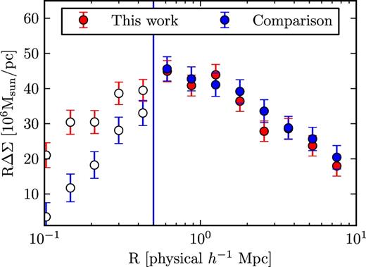
Lensing signal from the redMaPPer catalogue for our analysis (‘this work’) and the comparison ESS catalogue (‘comparison’). We consider the signals comparable at all scales ≥500 h−1 kpc. Filled circles are comparable data points, while open circles are shown for scales smaller than the cut-off.
In our work, we have corrected for dilution of the source sample by cluster member galaxies under the assumption that cluster member galaxies have zero shear. If cluster member galaxies are radially aligned, however, our correction will be underestimated. Blazek et al. (2012) tried to measure the radial intrinsic alignment (IA) signal of galaxies in our source sample with respect to the positions of luminous red galaxies (LRGs) at a similar redshift to our clusters. They were unable to detect an IA signal, placing an upper limit of 1.5 per cent on the fractional contamination of IAs on the recovered galaxy–galaxy lensing signal at a separation of 1 h−1 Mpc. To estimate an upper limit for this work, we must consider two factors: differences in the IA strength, and differences in the ΔΣ (which will modify the fractional contamination estimate). To estimate the former, we use the fact that the IA strength depends on the type and luminosity of the source galaxies (which is the same in this work and that one), and on the density tracers used as lenses. Singh, Mandelbaum & More (2015) provide an empirically determined power-law relationship between the small-scale IA strength and the halo mass of the density tracer, which we can use to scale up the estimated IA. After taking into account the increase in lensing signal ΔΣ between our clusters and LRGs, we find that the 1.5 per cent upper limit on fractional contamination for LRG lenses corresponds to an ≈6 per cent upper limit for galaxy clusters. While this upper limit is comparable to our uncertainties, we note that IA remains undetected for typical satellite galaxy populations in galaxy clusters (e.g. Sifón et al. 2015), with detections only for LRGs (e.g. Singh et al. 2015). For the purposes of this work, we have chosen not to increase our systematic error budget, pending future investigations of IAs in galaxy clusters. Indeed, these arguments suggest that IA may soon become an important systematics that must be simultaneously fit for when analysing stacked cluster lensing data (unless all galaxies at or very near the cluster redshift can be robustly removed).
5.2 Cluster miscentring
The likelihood of each of the combined data sets (XCS and ACCEPT) is the product of the probability P(R) over the clusters in the joint cluster samples. The resulting constraints are summarized in Table 2, where we report the mean and standard deviation of the parameters computed from the MCMC. We do not report on the posterior of the parameter R0 since it is purely a nuisance parameter for this study.
Constraints on the miscentring parameters from each of the various external data sets. The ‘number’ column refers to the total number of clusters in the sample. The parameter f is the fraction of miscentred clusters; the parameter τ characterizes the width of the centring offset distribution of miscentred clusters.
| External data set | Number | f | τ |
|---|---|---|---|
| XCS | 82 | 0.85 ± 0.05 | 0.48 ± 0.09 |
| ACCEPT | 54 | 0.75 ± 0.06 | 0.31 ± 0.05 |
| External data set | Number | f | τ |
|---|---|---|---|
| XCS | 82 | 0.85 ± 0.05 | 0.48 ± 0.09 |
| ACCEPT | 54 | 0.75 ± 0.06 | 0.31 ± 0.05 |
From Table 2, we see that the two high-resolution X-ray data sets are consistent with each other and with our expectation f = 87 per cent. We consider two analyses: one in which the miscentring priors are chosen following a ‘middle-of-the-road’ approach, with a Gaussian prior f = 0.80 ± 0.07 and τ = 0.40 ± 0.1, and one for which the miscentring fraction is set to the expected value f = 0.87 based on the redMaPPer centring probabilities. We note that from the summary of our binning scheme in Table 1 one can see that the reported fraction f from the redMaPPer algorithm itself is roughly constant for all λ and redshift bins, so we do not include further richness or redshift evolution in this parametrization beyond what is implied by the dependence of miscentring radius on the cluster radius.
5.3 Cluster projections
Photometric cluster finding is known to suffer from projection effects. That is, two neighbouring clusters that fall along the line of sight will be blended by the photometric cluster finder into a single, apparently larger cluster. We estimate the projection rate in the redMaPPer cluster catalogue to be p = 10 ± 4 per cent (see Appendix C). Characterizing the impact of such projections on cluster mass calibration is not trivial, but rough scalings can be readily estimated. In particular, clusters that appear in projection will also have a lensing signal affected by said projection effects. If the richness λ scales roughly linearly with the mass M, then the total projected mass per unit richness will remain constant, implying that projected clusters simply slide up and down the richness mass relation, without deviating from it. Indeed, this effect has been seen in numerical simulations (Angulo et al. 2012; Noh & Cohn 2012). Below, we quantify this effect in a way that can be incorporated into our analysis.
5.4 Cluster triaxiality
Dark matter haloes are known to be triaxial. Optically selected haloes are expected to be biased so that they are preferentially elongated along the line of sight. In this case, the galaxy contrast relative to the immediate neighbourhood should be maximized, making cluster detection easier. The elongation of the halo along the line of sight will naturally lead to an enhanced weak lensing signal, and so the recovered mass–richness relation may well be affected by this type of selection effect. For our purposes, the key point is that cluster triaxiality induces covariance between cluster richness and weak lensing mass estimates.
5.5 Modelling systematics
Recent work indicates that the more flexible Einasto profile (three free parameters; Einasto 1965; Dutton & Macciò 2014) may describe dark matter haloes more accurately than our assumed NFW profile. Depending on the details of the weak lensing analysis, the differences between Einasto and NFW profiles can be significant. For instance, Sereno, Fedeli & Moscardini (2016) find biases from fitting NFW profiles to Einasto haloes that range from −1 per cent for low- and middling-mass clusters to ∼+15 per cent for the highest mass clusters. However, these biases come from fits that use smaller radii (by a roughly a factor of 2) than the smallest radial bin considered in this study. The biases we see should be less, since the difference between NFW and Einasto profiles is largest at small scales; Mandelbaum, Seljak & Hirata (2008a) performed fits over a radius range more similar to ours and found negligible differences in the masses and moderate differences in the concentrations. Therefore, we do not expect to see such large biases because of the modest range of scales we probe. Nevertheless, the main point stands: one should check whether the profile assumed induces a significant bias in the weak lensing mass estimate. This is especially true in our case, since we rely on an NFW halo out to scales comparable to the splashback radii of our haloes, where one expects systematic deviations from the NFW profile (Diemer & Kravtsov 2014).
Here, we address this source of systematic uncertainty using numerical simulations to test whether our parametric models can introduce significant biases in our recovered weak lensing masses. Specifically, we use an N-body simulation with a volume V = [1.05 h−1 Gpc]3 and 2.7 billion particles, run with the l-gadget code, a variant of gadget (Springel 2005). The cosmological model is flat ΛCDM with matter density Ωm = 0.318, σ8 = 0.835, h = 0.670 and ns = 0.961. We use the halo catalogue generated by the rockstar halo finder (Behroozi, Wechsler & Wu 2013). In this simulation a 3.5 × 10¹³ h−1 M⊙ halo is resolved with 103 particles.
We construct synthetic weak lensing profiles from the numerical simulation. First, we divide the simulation into 64 jackknife regions. We assign an observed ‘richness’ to each halo in the simulation via λ = Mobs/1014 h−1 M⊙. Mobs is the effective observed mass of the halo, computed via ln Mobs = ln Mtrue + δ where δ is a Gaussian random draw of zero mean and variance 〈δ2〉1/2 = 0.2, intended to model lognormal scatter in the mass–observable relation. Clusters are sorted into richness bins, and the lensing profiles for these bins are fit using our likelihood model with no miscentring. We change the Ωm of our model-fitting pipeline to the value from the simulations for these tests only. We adopt the same mass–richness relation model as equation (12), this time with pivot λ = 1, and we allow for lognormal scatter in mass at fixed richness. We use the data error bars to replicate our sensitivity to different radius scales, and combine the results from the 64 jackknife samples to measure any potential bias at a higher precision than the data error bars would allow from any one fitting procedure alone.
Using the formalism in Evrard et al. (2014), the resulting best-fitting M0 value should be |$\log M_0 = 14.0 - \beta \sigma _{M|\lambda }^2/\ln (10) = 13.953 \pm 0.006$|, where β is the slope of the halo mass function over the range of halo masses probed. The error bar in our theoretical predictions comes from the difference between the first- and second-order calculation using the formalism of Evrard et al. (2014). We compare this expectation against our recovered M0 values to characterize the systematic uncertainty Δlog M0 associated with our parametric modelling. We find results consistent with our expected value, 13.953 ± 0.001 if we use all simulation mass bins or 13.943 ± 0.004 if we use only the bins within our expected observational mass range. As the error bar is dominated by the theoretical uncertainty, we choose to add no further uncertainty to our error budget based on this comparison.
5.6 Baryonic effects
Baryonic physics may modify the matter density profile of haloes relative to that observed in dark-matter-only simulations. Simulations that include baryonic cooling as well as active galactic nuclei (AGN) feedback have been used to study the impact of baryons on halo profiles (e.g. Schaller et al. 2015; Bocquet et al. 2016; Cui et al. 2016b). We summarize the trends in these papers as follows. First, on very small scales, the stellar mass component of the central galaxy dominates. These scales are excluded from our analysis. At somewhat larger scales, the profiles become either more or less concentrated depending on the relative impact of baryonic cooling to AGN feedback. The haloes are still roughly NFW, but the scale radius rs changes, reflecting the overall mass redistribution within a halo. The fact that we marginalize over a rescaling of the concentration–mass relation should allow us to avoid substantial biases in mass estimates due to the change in halo concentrations. Thirdly, and most importantly for our purposes, the mass within R200m is very stable, well below the 5 per cent level. As such, we expect the impact of baryons is well below our final error budget, and is therefore ignorable. Nevertheless, we caution that the impact that baryonic physics has on M200m is likely to become relevant to future weak lensing experiments. Fortunately, a straightforward generalization of the calibration program detailed above relying on simulations with baryonic physics should easily allow us to incorporate such systematics in future analyses.
5.7 Systematics summary
The systematics we consider are: shear and source photometric redshift systematics (±5 per cent in ΔΣ), cluster projections, halo triaxiality (combined −2 ± 3 per cent in M0) and modelling systematics (no additional uncertainty). We handle the ΔΣ errors via marginalizing over the fitting parameter b as described in Section 4.3; we note that this is a 5 per cent top-hat prior, which when combined with other Gaussian errors should contribute approximately 3.5 per cent to a Gaussian uncertainty on the overall amplitude. We apply the errors and bias correction in M0 due to halo triaxiality and halo projections a posteriori to our measured mass amplitude from our fitting procedure.
In the previous sections, we specified miscentring priors, but we did not estimate how miscentring impacted the uncertainty in the recovered weak lensing mass. To test this, we compare the results of our fiducial analysis to a second analysis in which the miscentring parameters are held fixed at their fiducial values. We find the resulting uncertainties in the amplitude of the mass–richness relation are essentially identical, so cluster miscentring does not appear to have a significant impact on the precision of weak lensing mass calibration. It does, however, impact the uncertainties in concentration. In short, current miscentring estimates are sufficiently accurate to be negligible for mass calibration purposes, but not for analyses of the mass–concentration relation.
Since we have included our systematic uncertainties in the outputs of the MCMC chains themselves, we cannot distinguish systematic from statistical errors in this calculation. To obtain a statistical error, we run a separate chain with all the nuisance parameters (b, the miscentring parameters, and our bias correction) fixed to their central values, with no uncertainty included, and measure the statistical error from the uncertainty in the resulting parameters. We subtract this in a quadrature from the total systematic plus statistical uncertainty to obtain the systematic uncertainty.
6 RESULTS
Fig. 2 shows the results from our MCMC fitting procedure. We obtain a fit with |$-2 \ln {\cal {L}}=76.37$|, which would (without our priors) correspond to a χ2 value for 72 degrees of freedom. That is, our model is a good fit to the data. A sampling of the models from our chains along with our data can be seen in Fig. 3. Table 3 reports our model parameters, along with the corresponding priors and posteriors. We note that the amplitude and slope of the mass–richness scaling relation, as well as the amplitude of the mass–concentration relation, are tightly constrained. Our constraint on the amplitude of mass–richness relation parameter is log M0 = 14.344 ± 0.021 (statistical) ±0.023 (systematic), corresponding to a 7 per cent calibration of the amplitude of the scaling relation. The corresponding constraint on the power-law index of the mass–λ relation is |$\alpha = 1.33^{+0.09}_{-0.10}$|. The posterior probability for the scatter in the mass–richness relation and the miscentring probability are largely unchanged from the input priors, demonstrating that the external data sets utilized to derive the priors are significantly more sensitive to these parameters than the stacked weak lensing signal measured in this work.
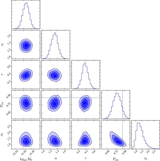
Results from our MCMC model fitting. Contours indicate the 0.5, 1, 1.5 and 2σ levels, and the one-dimensional histograms are shown on the diagonal. The range shown for each parameter does not necessarily correspond to the top-hat prior ranges. Parameters and priors are described in Table 3. The solid line denotes the expected value of 〈Pcen〉 = 0.87 from the redMaPPer catalogue.
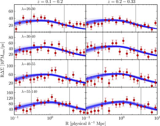
Lensing signal (RΔΣ) from the redMaPPer catalogue for the eight bins described in Table 1, plus a sampling of models from the MCMC chain. The fit was performed only to data points lying between the vertical lines.
Parameters from equations (12) and (19), a short description of the meaning, the prior and the median of all MCMC samples plus the errors given by the 16th and 84th percentiles of the samples. M0 has been corrected from the output of the MCMC chain for model bias, as described in Section 5. We also show the results if we fix Pcen to 0.87, the mean value from the redMaPPer catalogue centring probabilities. A range means a top-hat prior; |$\mathcal {N}(x,\sigma )$| is a Gaussian prior with mean x and width σ. For posteriors with two uncertainties given, the first is statistical and the second is systematic.
| Parameter | Description | Prior | Median and error | Median and error |
|---|---|---|---|---|
| (posterior) | (Pcen = 0.87) | |||
| log10M0 | Log amplitude of scaling relation at λ0 = 40 | (13, 15) | 14.344 ± 0.021 ± 0.023 | 14.338 ± 0.021 ± 0.021 |
| in units of h−1 M⊙, with definition M200m | ||||
| α | Power-law index of dependence on λ | (0, 2) | |$1.33^{+0.09}_{-0.10}$| | 1.34 ± 0.09 |
| σln M|λ | Intrinsic scatter of λ–M relation | (0.2, 0.3) | 0.25 ± 0.03a | 0.25 ± 0.03a |
| c0 | Amplitude of mass–concentration relation | [0, 3) | |$1.34^{+0.35}_{-0.25}$| | |$1.11^{+0.16}_{-0.14}$| |
| as a multiple of Bhattacharya et al. (2013) | ||||
| τ | Width of the Gaussian miscentring distribution | |$\mathcal {N}(0.4,0.1)$| | 0.37 ± 0.08a | 0.38 ± 0.09a |
| Pcen | Fraction of clusters with correct centres | |$\mathcal {N}(0.80,0.07)$| | 0.77 ± 0.07a | – |
| b | Multiplicative amplitude shift to accommodate | (−0.05, 0.05) | 0.00 ± 0.03a | 0.00 ± 0.03a |
| systematic errors in ΔΣ |
Note.asymbol indicates values that are largely determined by our priors rather than our data.
There is a degeneracy between Pcen and the amplitude of the mass–concentration relation, which is unsurprising, as both parameters correspond to shifts in the ‘peakiness’ of the profile. τ is not included in this degeneracy, but shifts in τ have a smaller effect on the profile since Pcen is large.
We do not show the parameters σln M|λ or b, which are unconstrained by the data. σln M|λ is not degenerate with any other parameter, and we find no preference for any value within our top-hat prior range. We also find no preference for any value of b. Not surprisingly, we find that b is degenerate with the mass, with the mass scaling as 10−b/2 for our fits. Also, b is degenerate with the concentration amplitude c0, with c0 ∝ 1 − b.
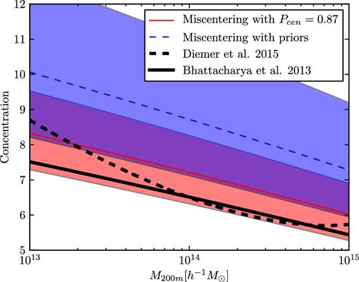
In Fig. 4, we show how our fitted mass–concentration relation compares to two theoretical models, Bhattacharya et al. (2013) and Diemer & Kravtsov (2015). We also show the mass–concentration relation recovered when we fix Pcen to the value expected from the redMaPPer catalogue, 0.87. In both cases, we find somewhat higher values of c than the theoretical models predict, but the difference is only 1σ and hence not statistically significant. Appendix B also demonstrates that allowing for redshift evolution in the mass–richness relation does not alter any of our conclusions. In Appendix A we show results with and without various complicating factors (such as miscentring and a variable mass–concentration relation), to aid comparison with other works and to show the effects of those factors for interested readers.
Because the halo mass definition is dependent on cosmology, our results change if we alter Ωm. We perform the same analysis as above with Ωm from 0.26to0.34 to check the dependence of our parameters on cosmology, altering ΩΛ as well to maintain a flat universe. Only the mass amplitude changes, as expected; we find that log10M0 is linear with Ωm near Ωm = 0.3, with the scaling log10M0 = 14.344 − 0.706(Ωm − 0.3). As expected, M0 decreases as Ωm increases.
7 DISCUSSION
We compare our results to a variety of constraints from the literature. The first mass–richness relation for redMaPPer clusters was a rough abundance-matching estimate presented in Rykoff et al. (2012), who suggested a scaling relation with α = 1.08 and M = (3.9 ± 1.2) × 1014 h−1 M⊙ at λ = 60, in excellent agreement with our recovered value of (3.7 ± 0.3) × 1014 h−1 M⊙. There is an apparent slight tension (2.5σ) in the value of the slope, but Rykoff et al. (2012) did not report an uncertainty in the slope. We note that Rykoff et al. (2012) emphasized their reported relation was only meant to be a place holder for subsequent mass calibration efforts such as this one.
Miyatake et al. (2016) used the same SDSS weak lensing shear catalogue and photo-z catalogue and calibration as we did to constrain the mean mass of entire redMaPPer cluster catalogue. Despite the shared input data set, there are significant methodological differences between the two analyses. In particular, our science goal led us to provide a much more detailed systematics analysis than that presented in Miyatake et al. (2016). The end mass calibrations are, perhaps not surprisingly, very similar. Our principal contribution is the quantitative characterization of the systematic uncertainties inherent to this measurement, as well as determination of the scaling of mass with λ instead of just a population average.
Li et al. (2016) produced a weak lensing calibration of the mass–richness relation as a by-product of their analysis on the lensing profile of cluster substructures. Specifically, they assume a mass–richness relation that was identical to that of Rykoff et al. (2012), except modulated by an amplitude A. This amplitude is allowed to float when considering substructures in different radial bins. We combine the various radial bins, ignoring the innermost bin because it is discrepant with the rest of the data, and is the bin most likely to be affected by systematic uncertainties from magnification, non-weak shear and source obscuration. Averaging the Li et al. (2016) data results in A = 0.803 ± 0.016, corresponding to M = (2.09 ± 0.04) × 1014 h−1 M⊙ at λ = 40. This value is in excellent agreement with our recovered value of M = (2.21 ± 0.15) × 1014 h−1 M⊙. We note the error quoted in Li et al. (2016) is statistical only.
Recent work by Farahi et al. (2016) has calibrated the mass–richness relation of redMaPPer clusters using stacked velocity dispersion information. They report M200c = (1.56 ± 0.35) × 1014 M⊙ at λ = 30 with h = 0.7. This can be compared to our prediction M200c = (1.60 ± 0.11) × 1014 M⊙, in excellent agreement with their result. The corresponding slopes are also in excellent agreement, |$\alpha =1.33^{+0.09}_{-0.10}$| in our analysis, and α = 1.31 ± 0.14 in theirs.
Saro et al. (2015, hereafter referred to simply as Saro) calibrated the richness–mass relation for redMaPPer clusters in the Dark Energy Survey (DES) Science Verification data by cross-matching DES redMaPPer clusters to clusters found by the South Pole Telescope (SPT; Bleem et al. 2015). The SPT clusters were assigned masses by assuming that the SPT cluster abundance is consistent with a flat ΛCDM cosmology with Ωm = 0.3 and σ8 = 0.8. In this way, the SPT clusters are assigned both a mass – for which they utilized M500c – and a richness, allowing Saro to infer the cluster richness–mass relation. Using the framework of Evrard et al. (2014), the corresponding mass–richness relation can be written as 〈M500c|λ〉 = (3.2 ± 0.6) × 1014 h−1 M⊙ at λ = 66.1, the pivot richness for their sample. The above value is corrected for the predicted redshift evolution between the Saro redshift pivot point and ours, using the Saro constraints on the evolution of the mass–richness relation, and the corresponding uncertainty has been adequately propagated. We convert our predicted masses from M200m to M500c following Hu & Kravtsov (2003) and the Bhattacharya et al. (2013) mass–concentration relation to arrive at a predicted mass M500c = (2.2 ± 0.15) × 1014 h−1 M⊙, in reasonable agreement (1.6σ) with the Saro value. Despite the apparent disparity in the central values for the slopes of the mass–richness relation – Saro find α = 0.91 ± 0.18, compared to our value |$1.33^{+0.09}_{-0.10}$| – the two values are consistent at the 2σ level. We note that the above comparison assumes there is no systematic offset in the richness measurements of a galaxy cluster between the SDSS and DES data sets, an assumption that is currently not testable. Indeed, the agreement between the two measurements could be interpreted as evidence that there are no large systematic differences in the richness between the two data sets, as suggested by a comparison of their relative abundances (Rykoff et al. 2016).
Our miscentring values are largely controlled by our priors, as we do not have as much constraining power with the weak lensing only due to degeneracies between parameters that modify the profile shape. We can compare these miscentring parameters to previous results as well. Our lensing-weighted average Rλ is 0.79, so our miscentring τ corresponds to approximately Rmis = 0.29 ± 0.06 h−1 Mpc. Rozo & Rykoff (2014) find offsets corresponding to constant probability out to Rmis = 0.8 h−1 Mpc. However, we note that their straight-line fit is in fact similar to the cumulative distribution function of the Rayleigh distribution we assume for our miscentring offsets. The constant probability out to Rmis = 0.8 h−1 Mpc that they find is approximately equivalent to a Rayleigh distribution with Rmis = 0.3 h−1 Mpc, very consistent with our results. Our peak value is smaller than the simulations of the MaxBCG cluster sample (Johnston et al. 2007b) of ∼0.4 h−1 Mpc, although as that catalogue uses different methods of finding the centre of a galaxy clusters, discrepancies should be expected. The RCS cluster sample has a well-measured miscentring width of 0.41 ± 0.01 h−1 Mpc for 1014 M⊙ haloes (van Uitert et al. 2016), in good agreement with our measurement of 0.43 ± 0.09 h−1 Mpc for the same haloes. Their fraction of correctly centred haloes is smaller, again reflecting differences in the cluster-finding algorithms or perhaps differences in the performance of the centroiding algorithm with redshift, as they include clusters up to z = 0.7.
As for the mass–concentration relation, our results appear to be in excellent agreement with theoretical expectations. We caution, however, that while our model accounts for projection effects, halo triaxiality and cluster miscentring with regards to calibrating the mass–richness relation, we have not performed a similar calibration for the impact on concentration. Indeed, a recent paper by Baxter et al. (2016), looking at the clustering of redMaPPer clusters, demonstrated that redMaPPer clusters tend to be preferentially more compact than randomly oriented haloes, an effect that would tend to bias our recovered parameter c0 to values larger than unity, exactly as observed. We postpone a detailed calibration of this effect, and therefore a more detailed comparison to numerical simulations and observational studies, to future work.
8 SUMMARY
We have measured the weak lensing signal around 5570 clusters in the redMaPPer catalogue from SDSS DR8, with richnesses 20 < λ < 140 and redshifts 0.1 < z < 0.33. The signal shows good agreement with a comparison signal calculated using the same cluster catalogue, but a different shape measurement pipeline and photo-z algorithm and pipeline.
The mass modelling method we use is an extension of previous work, such as the maximum-likelihood lensing approach adopted by Han et al. (2015) and the combination fits of Ford et al. (2014). The model makes it easy to self-consistently include a varying mass–concentration relation and scatter in the mass–richness and mass–concentration relations, as well as removing uncertainty from the question of which richness in a richness bin best corresponds to the mass value obtained from a single-halo fit. We test the model on N-body simulations and find excellent agreement with the true input cluster sample properties.
Including miscentring and a varying mass–concentration relation is important to obtaining accurate results with this sample in this radius range. That is, while our priors on cluster centring are sufficiently tight that miscentring does not contribute a significant fraction of the variance in our mass calibration, we find that ignoring centring outright would result in a 0.3σ systematic shift in the slope of our mass–richness relation towards higher values.
The results in this work provide the most careful weak lensing mass calibration analysis of the redMaPPer cluster catalogue to date, with a detailed budget of systematic uncertainties and null tests. This is also the first time that a cluster mass calibration effort has included a null test comparing two independently developed photo-z and shear codes as a way to validate the estimated systematic uncertainties in the recovered halo masses. Our results provide a critical stepping stone towards placing cosmological constraints with the redMaPPer cluster sample, and pave the way for similar analyses in upcoming photometric survey data, such as that of the DES, HSC and LSST surveys.
Acknowledgments
The authors thank Bhuvnesh Jain and Eric Baxter for useful discussions related to this work. MS and RM acknowledge the support of the Department of Energy Early Career Award program. ES is supported by DOE grant DE-AC02-98CH10886. This work received partial support from the US Department of Energy under contract number DE-AC02-76SF00515 and from the National Science Foundation under NSF-AST-1211838. We thank Mathew Becker and Michael Busha for their contributions to the N-body simulations used in this work.
Funding for SDSS-III has been provided by the Alfred P. Sloan Foundation, the Participating Institutions, the National Science Foundation and the US Department of Energy Office of Science. The SDSS-III web site is http://www.sdss3.org/.
SDSS-III is managed by the Astrophysical Research Consortium for the Participating Institutions of the SDSS-III Collaboration including the University of Arizona, the Brazilian Participation Group, Brookhaven National Laboratory, Carnegie Mellon University, University of Florida, the French Participation Group, the German Participation Group, Harvard University, the Instituto de Astrofisica de Canarias, the Michigan State/Notre Dame/JINA Participation Group, Johns Hopkins University, Lawrence Berkeley National Laboratory, Max Planck Institute for Astrophysics, Max Planck Institute for Extraterrestrial Physics, New Mexico State University, New York University, Ohio State University, Pennsylvania State University, University of Portsmouth, Princeton University, the Spanish Participation Group, University of Tokyo, University of Utah, Vanderbilt University, University of Virginia, University of Washington and Yale University.
Present address: Department of Physics, Astronomy, University of California, Riverside, CA 92507, USA.
An updated version of the software that was used to produce this catalogue is publicly available as part of the GalSim package (Rowe et al. 2015): https://github.com/GalSim-developers/GalSim
The difference is merely a parametrization choice – a shear is a ratio of linear functions of the axis ratio of the ellipse, while a distortion is a ratio of functions of the axis ratio squared.
To address a possible source of confusion, the Evrard et al. (2014) framework uses α to denote the power-law slope of parameters given mass; i.e. to zeroth-order, our α, denoting the power-law slope of mass given λ, is the inverse of theirs.
Here, obscuration refers not only to the literal blocking of source galaxies by member galaxies, but also the inability to properly select them due to blending with member galaxies. This is sometimes called crowding.
REFERENCES
APPENDIX A: Details of |$\boldsymbol {\Delta \Sigma }$| model components
Our final model includes marginalization over multiple modelling issues that are secondary to the relationship we are primarily interested in measuring. We show here a simple model including none of them, and then add more complications one at a time, to better show the effect each additional parameter has on our final results. Table A1 shows the results for our MCMC model fitting for different combinations of parameters. We discuss here the various complications of the model.
Fitting results for all of our cluster models, showing the parameters of scientific interest only. We report the settings for the MCMC chain and the maximum likelihood |$-2\ln {\cal {L}}$| of any step in any chain for that MCMC run. We run the emcee MCMC ensemble sampler with 100 walkers for every chain, so the total number of steps included in the plots is 100 times what is listed here (including burn-in steps). When the Gaussian priors are not important, |$-2\ln {\cal {L}}$| is equal to the χ2. We also report the median value and the 1σ error regions (the 16th–84th percentile range) for the parameters of scientific interest. All models are NFW (equation 8), some with miscentring (equation 11), some with fitted M–c relations. The last model in the table is our fiducial model used in the analysis in the main text of this work. The * symbol indicates that the mass values from the output of the MCMC chain have been corrected for model bias, as described in Section 5, and the error bar is combined statistical and systematic.
| No. of steps | Minimum | ||||
|---|---|---|---|---|---|
| Model name | (burn-in) | |$-2\ln {\cal {L}}$| | d.o.f. | |$\log _{10} M_0^{\ast }$| | α |
| Simple | 1000 (100) | 78.41 | 75 | |$14.322^{+0.028}_{-0.029}$| | |$1.36^{+0.10}_{-0.09}$| |
| Simple with M–c scatter | 1000 (100) | 78.09 | 75 | |$14.323^{+0.028}_{-0.029}$| | |$1.36^{+0.09}_{-0.10}$| |
| Fitted M–c amplitude and M–c scatter | 1500 (100) | 77.64 | 74 | 14.329 ± 0.030 | |$1.38^{+0.09}_{-0.10}$| |
| Miscentring and M–c scatter | 1500 (100) | 78.08 | 73 | 14.347 ± 0.030 | |$1.36^{+0.09}_{-0.10}$| |
| Miscentring, fitted M–c amplitude and M–c scatter | 2250 (100) | 76.37 | 72 | 14.344 ± 0.031 | |$1.33^{+0.09}_{-0.10}$| |
Our simple model assumes no miscentring and a mass–concentration (M–c) relation from the literature, Bhattacharya et al. (2013), evaluated using the publicly available colossus package described in Diemer & Kravtsov (2015), without M–c scatter. The values we obtain for the parameters, shown in Table A1, already have many of the characteristics we see in the final analysis: log M0 is somewhat above 14 and α well above 1. Our parameter values do not change significantly when we add the various complications: lognormal scatter in the mass–concentration relation with width 0.14 dex as described in the main text; a variable mass–concentration relation; miscentring; and all three. There is a ∼0.3σ decrease in α when we include all effects versus all other models, indicating that a small amount of the apparent scaling of mass with λ in the simple model can be attributed to those effects changing with the cluster richness, but the effect is small. The nuisance parameters (b and miscentring) are largely determined by our priors; c0, the amplitude of the mass–concentration relation, shows more movement, with a value of |$0.90^{+0.12}_{-0.10}$| when there is no miscentring included but |$1.34^{+0.35}_{-0.25}$| when it is. Adequate modelling of the miscentring is clearly important for weak lensing studies such as these which attempt to measure the M–c relation using information at scales less than the miscentring radius.
The fit quality does not vary strongly with the inclusion of more parameters, as judged by the best-fitting likelihood. In summary, we can fit the redMaPPer cluster lensing signal reasonably well with a sum of NFW profiles that have characteristics determined by the input λ and redshift distribution of the redMaPPer catalogue. For the radius range and cluster distribution included in this work, including higher level complications such as miscentring and variable mass–concentration relations is not important to obtaining a reliable mass amplitude, but do affect the scaling with richness to some extent.
APPENDIX B: REDSHIFT EVOLUTION
The value preferred for β, −1.5 ± 0.9, is consistent with our expected value of 0 at slightly above 1.5σ. The fit is better, with the minimum |$-2 \ln {\cal {L}}=76.64$| instead of 78.41, but no other parameter moves significantly when β is included. Since we expect β ≈ 0 and cannot exclude this possibility using the data, we do not include redshift evolution of the mass–λ relation in the model used for our main results in this paper. Fixing β = 0 is a stronger assumption than letting β float with some prior on expected values; however, we know what fixing β = 0 does (finds the average value over all redshifts) while it is unclear what we would be modelling if we allowed β to float, so we make the trade-off of being insensitive to redshift in favour of better understanding the physical importance of our other parameters.
APPENDIX C: THE PROJECTION RATE IN THE redMaPPer CLUSTER CATALOGUE
In Section 5.3, we estimated the impact of projection effects on our weak lensing mass calibration. Our starting point in that section was the projection rate in the redMaPPer cluster catalogue. Here, we discuss how we arrived at the prior for this projection rate.
Our starting point is Rykoff et al. (2014), who set a lower limit on the incidence of these type of projection effects by placing synthetic galaxy clusters within the SDSS survey and then performing a cluster finding step. We found a richness-dependent rate of projection effects that increases with richness, reaching 5 per cent for the richest clusters.
On the basis of these arguments, we adopt a projection rate p = 10 ± 4 per cent.
