Merger-driven evolution of the effective stellar initial mass function of massive early-type galaxies

Sonnenfeld, Alessandro; Nipoti, Carlo; Treu, Tommaso

doi:10.1093/mnras/stw2919

Abstract

The stellar initial mass function (IMF) of early-type galaxies is the combination of the IMF of the stellar population formed in situ and that of accreted stellar populations. Using as an observable the effective IMF α_IMF, defined as the ratio between the true stellar mass of a galaxy and the stellar mass inferred assuming a Salpeter IMF, we present a theoretical model for its evolution as a result of dry mergers. We use a simple dry-merger evolution model, based on cosmological N-body simulations, together with empirically motivated prescriptions for the IMF to make predictions on how the effective IMF of massive early-type galaxies changes from z = 2 to z = 0. We find that the IMF normalization of individual galaxies becomes lighter with time. At fixed velocity dispersion, α_IMF is predicted to be constant with redshift. Current dynamical constraints on the evolution of the IMF are in slight tension with this prediction, even though systematic uncertainties, including the effect of radial gradients in the IMF, prevent a conclusive statement. The correlation of α_IMF with stellar mass becomes shallower with time, while the correlation between α_IMF and velocity dispersion is mostly preserved by dry mergers. We also find that dry mergers can mix the dependence of the IMF on stellar mass and velocity dispersion, making it challenging to infer, from z = 0 observations of global galactic properties, what is the quantity that is originally coupled with the IMF.

stars: luminosity function, mass function, galaxies: elliptical and lenticular, cD, galaxies: evolution, galaxies: stellar content

1 INTRODUCTION

Understanding the properties and the origin of the stellar initial mass function (IMF) is currently one of the biggest challenges in galaxy formation theory. Observational constraints on the IMF provide us with a puzzling scenario. On one hand, the IMF appears to be remarkably self-similar across different environments within the Milky Way (see e.g. Bastian, Covey & Meyer 2010; Offner 2015). On the other hand, the IMF in early-type galaxies is inferred to vary systematically as a function of mass or velocity dispersion (Treu et al. 2010; Cappellari et al. 2012; Conroy & van Dokkum 2012; Dutton, Mendel & Simard 2012; Tortora, Romanowsky & Napolitano 2013; Spiniello et al. 2014; Posacki et al. 2015), although even for massive early-type galaxies, we are still far from a clear picture (Smith, Lucey & Conroy 2015). Efforts have been put into reproducing from a theoretical standpoint the observed IMF trends. However, despite recent progress (Hennebelle & Chabrier 2011; Krumholz 2011; Hopkins 2012; Guszejnov, Krumholz & Hopkins 2016), we still lack a coherent description of star formation across all environments.

One complication in comparing measurements of the IMF with models is that present-day stellar populations are ensembles of stars formed at different epochs in a range of environments. For massive early-type galaxies, a significant fraction of their present-day stellar mass is believed to be accreted from other systems (e.g. van Dokkum et al. 2010). If the IMF is not universal, then each accreted object will in general have a different IMF from the pre-existing population of the central galaxy. The IMF of a massive galaxy at z = 0 will then be the combination of the IMF of the stellar population formed in situ and that of the accreted galaxies, possibly resulting in spatial gradients (Martín-Navarro et al. 2015a; La Barbera et al. 2016). How does this ‘effective’ IMF evolve in time? Answering this question and comparing the predictions to observations provides a new way to test galaxy formation and star formation models.

While the IMF is typically assumed as universal in cosmological simulations, there are studies of galaxy evolution based on semi-analytical models (SAMs) that allow for a non-universal IMF (Nagashima et al. 2005; Bekki 2013; Chattopadhyay et al. 2015; Gargiulo et al. 2015a; Fontanot et al. 2016). These works explore mostly the effect of the IMF on the chemical evolution of galaxies.

In order to isolate the effects of a varying IMF in the context of dry mergers, we adopt a simple model based on cosmological numerical simulations, galaxy–galaxy mergers simulations, and empirical prescriptions for the varying IMF. In practice, we use a simple prescription for assigning the starting (z = 2) IMF of an ensemble of galaxies and then evolve the stellar population of central galaxies by merging their stellar content with that of accreted satellites. We tune our model to match the correlation between IMF normalization and stellar mass observed at z ∼ 0 and use it to make predictions on the stellar IMF of massive galaxies at higher redshifts. Though very simple in its construction, our model allows us to clearly isolate the effect of dry mergers, which are believed to represent the main growth mechanism of massive early-type galaxies at z < 2, on the evolution of the IMF.

The paper is organized as follows. In Section 2, we describe our model for the IMF of z = 2 galaxies and its evolution as a result of dry mergers. In Section 3, we present low-z measurements of the IMF used to calibrate our model. In Section 4, we show our predictions on the time evolution of the IMF. We discuss our results in Section 5, while Section 6 concludes. We assume a flat ΛCDM cosmology with H₀ = 70 km s⁻¹ Mpc⁻¹ and Ω_M = 0.3. Throughout the paper, velocity dispersions are expressed in units of km s⁻¹ and masses in units of M_⊙.

2 THE MODEL

2.1 Parameters and notation

Throughout our work, we use the following quantities to describe the stellar content of our galaxies. We first define a true stellar mass, |$M_{\ast }^{\mathrm{true}}$|⁠. Then, we introduce a Salpeter (Salpeter 1955) stellar mass, |$M_{\ast }^{\mathrm{Salp}}$|⁠, defined as the stellar mass one would infer by fitting a stellar population synthesis model based on a Salpeter IMF to broad-band photometric data. This quantity is typically used when observationally measuring stellar masses. We then consider the IMF mismatch parameter (Treu et al. 2010)

\begin{equation} \alpha _{\mathrm{IMF}}= \frac{M_{\ast }^{\mathrm{true}}}{M_{\ast }^{\mathrm{Salp}}}. \end{equation}

(1)

Stellar populations with a more bottom-light IMF than a Salpeter IMF will have α_IMF < 1. A Chabrier IMF for example corresponds typically to a value α_IMF ≈ 0.6. As defined above, α_IMF is a well-defined quantity also for galaxies that are characterized by multiple stellar populations with different IMFs, for example as a result of mergers. For typical cases, α_IMF is mostly sensitive to the behaviour of the IMF at small masses, which dominate the mass budget but contribute little to the light. Depending on the parametrization, it can be a probe of low-mass cutoff, and/or shape of the IMF. In extreme cases, α_IMF can be affected by the IMF at high masses, which, however, leaves an imprint not only on the mass-to-light ratio but also on other phenomena, such as metal enrichment or supernovae rates. In this work, α_IMF is the only parameter used to describe the IMF of a galaxy. Throughout our analysis, we identify the terms effective IMF and IMF normalization with this quantity.

In addition to the stellar mass of a galaxy, we track its halo mass M_h and its central stellar velocity dispersion σ: |$M_{\ast }^{\mathrm{true}}$|⁠, |$M_{\ast }^{\mathrm{Salp}}$|⁠, M_h, and σ are the only quantities that enter our model.

2.2 The mock sample

We generate a sample of 10 000 haloes at z = 2 with masses drawn from the halo mass function described by Tinker et al. (2008), using an upper cutoff at log M_h/M_⊙ < 13.5. We make this cut to focus on the regime of galaxy or galaxy group scale haloes, where most observational constraints on the IMF are measured (Gavazzi et al. 2007), excluding cluster of galaxy environments (though IMF constraints are available for some brightest cluster galaxies; Newman et al. 2013). We then assign a Salpeter stellar mass to each halo using the stellar-to-halo mass relation (SHMR) from Leauthaud et al. (2012), including scatter. The Leauthaud et al. (2012) SHMR is originally expressed in terms of stellar masses calculated assuming a Chabrier IMF. For massive red galaxies, the assumption of a Salpeter IMF in stellar population synthesis measurements produces stellar masses larger than Chabrier by 0.25 dex, with negligible scatter (Auger et al. 2010b). Therefore, we obtain an SHMR in terms of |$M_{\ast }^{\mathrm{Salp}}$| by applying the transformation

\begin{equation} \log {M_{\ast }} \rightarrow \log {M_{\ast }} + 0.25 \end{equation}

(2)

to the Leauthaud et al. (2012) SHMR.

We make an additional cut in stellar mass keeping only galaxies with |$\log {M_{\ast }^{\mathrm{Salp}}/\mathrm{M}_{\odot }} > 10.5$| and then select a random sample of 100 objects. Finally, we assign central stellar velocity dispersions σ assuming a power-law scaling with stellar mass,

\begin{equation} \log {\sigma } = \log {\sigma _0} + \beta _\sigma \left(\log {M_{\ast }^{\mathrm{Salp}}} - 11.5\right), \end{equation}

(3)

with log σ₀ = 2.48 and β_σ = 0.20 and a scatter of 0.05 in log σ. These values are such that the evolved population of mock galaxies reproduce the |$M_{\ast }^{\mathrm{Salp}}-\sigma$| relation measured at z ∼ 0 by Auger et al. (2010b, see Section 2.4).

2.3 The effective IMF

The effective IMF of massive galaxies has been shown to correlate with stellar velocity dispersion (e.g. Treu et al. 2010; Cappellari et al. 2012; Conroy & van Dokkum 2012; La Barbera et al. 2013; Spiniello et al. 2014; Posacki et al. 2015), stellar mass (Auger et al. 2010a; Sonnenfeld et al. 2015), and stellar-mass density (Spiniello et al. 2015). In light of these observations, we adopt a relation of the following form for assigning the IMF to our model galaxies at z = 2:

\begin{equation} \log {\alpha _{\mathrm{IMF}}} = a_{\ast }\left(\log {M_{\ast }^{\mathrm{Salp}}} - \mu _{\ast }\right) + a_\sigma (\log {\sigma } - \mu _\sigma ) + b, \end{equation}

(4)

where μ_* and μ_σ are the average logarithms of stellar mass and velocity dispersion of the sample. We then choose two different sets of values for the parameters a_*, a_σ, and b. In the first prescription, labelled ‘M_* model’, we set a_* = 0.26, a_σ = 0, and b = 0.21. For the second prescription, labelled ‘σ model’, we set a_* = 0, a_σ = 1.20, and b = 0.03. In other terms, the first model is a power-law relation between IMF and stellar mass, with no residual dependence on σ, while vice versa the IMF of the second model is set uniquely by the velocity dispersion. In each model, the values of the parameters have been tuned to approximately reproduce the low-z IMF measurements from S15. Details on these measurements are given in Section 3.

These prescriptions are purely empirically motivated. While there have been attempts at predicting the stellar IMF from first principles in terms of the global properties of a galaxy (e.g. Krumholz 2011; Hopkins 2012), implementing such models would require us to make additional assumptions on parameters of the star-forming gas such as the pressure and the turbulence Mach number. Given the current uncertainty on the true mechanism determining the IMF, the benefits of employing such theoretically motivated recipes are modest and we therefore limit our model to simpler empirical recipes.

2.4 The dry-merger evolution

Our central galaxies are evolved to z ∼ 0 using the dry-merger evolution model developed by Nipoti et al. (2012), with a few modifications. The method can be summarized as follows. For each central galaxy, we compute the evolution in its halo mass using the following expression from Fakhouri, Ma & Boylan-Kolchin (2010), which is derived from the Millennium I and II simulations:

\begin{equation} \frac{\mathrm{d}\ln {M_{\mathrm{h}}}}{\mathrm{d}z} = - \frac{\dot{M}_0}{10^{12}\,\mathrm{M}_{\odot } H_0}\frac{1 + fz}{1 + z}\left(\frac{M_{\mathrm{h}}}{10^{12}\,\mathrm{M}_{\odot }}\right)^{g-1}, \end{equation}

(5)

with |$\dot{M}_0 = 46.1 \mathrm{M}_{\odot } \rm {\, yr}^{-1}$|⁠, f = 1.11, and g = 1.1. In this step, we are assuming that the growth history of each halo in our sample is the same as the average growth history for haloes of the same mass. We separate the growth in halo mass into smooth accretion and growth due to mergers. We estimate the latter with the following expression from Fakhouri et al. (2010):

\begin{eqnarray} \frac{\mathrm{d}^2N_{\mathrm{merg}}}{\mathrm{d}z \mathrm{d}\xi }(z, \xi , M_{\mathrm{h}}) = A\left(\frac{M_{\mathrm{h}}}{10^{12}\,\mathrm{M}_{\odot }}\right)^\alpha \xi ^\beta \exp {\left[\left(\frac{\xi }{\tilde{\xi }}\right)^\gamma \right]}(1 + z)^{\eta ^{\prime }},\!\!\nonumber\\ \end{eqnarray}

(6)

which describes the number of mergers between haloes of mass ratio ξ per unit redshift interval. Following Fakhouri et al. (2010), we assume A = 0.0104, |$\tilde{\xi }=9.72\times 10^{-3}$|⁠, α = 0.133, β = −1.995, γ = 0.263, and η΄ = 0.0993. At each time-step dz, the change in halo mass due to mergers is then the integral over mergers of different halo mass ratios ξ,

\begin{equation} \!\left[\frac{\mathrm{d}M_{\mathrm{h}}}{\mathrm{d}z}\right]_{\mathrm{merg}} = -\int _{\xi _{\mathrm{min}}}^1 M_{\mathrm{h}}\xi \frac{\mathrm{d}^2N_{\mathrm{merg}}}{\mathrm{d}z \mathrm{d}\xi } \text{d}\xi . \end{equation}

(7)

We are assuming that only mergers with mass ratio larger than a minimum value ξ_min contribute. This minimum value is set by the merging time-scale: mergers with very small values of ξ have merging time-scales longer than the age of the Universe and therefore cannot contribute to the accreted mass. We fixed ξ_min = 0.03 following Nipoti et al. (2012). We tested for the impact of this choice on our study by varying ξ_min between 0.01 and 0.1 finding minimal differences in all the results, indicating that mergers with a halo mass ratio ξ > 0.1 are the most important in the growth of massive galaxies. This finding is in agreement with observational estimates of merger rates of massive galaxies, which find that the bulk of the accreted stellar mass is brought in by mergers with stellar mass ratio larger than 0.1 (Ferreras et al. 2014; Ruiz, Trujillo & Mármol-Queraltó 2014).

Another implicit assumption in our model is that, once accreted, the stellar mass of satellites is instantly added to that of the central galaxy. In reality, there should be a delay between the merger rate given by equation (6), which refers to the time at which accreted haloes become gravitationally bound to the central halo, and the rate at which stellar mass is added to the central galaxy. Such a delay is larger for minor mergers and depends on the merging orbital parameters (Boylan-Kolchin, Ma & Quataert 2008). The effects of this instantaneous merger approximation are however quite small. For instance, using the merger time-scale estimation of Nipoti et al. (2012), we find that among haloes accreted at z = 0.3, mergers with halo mass ratio ξ > 0.1 are expected to be completed by z = 0. Since mergers with a smaller mass ratio have a very little impact in our model, this indicates that effects of the delay are only relevant over a time-scale that is a small fraction of the time-frame considered in our study.

We then calculate the growth in Salpeter stellar mass assuming that each accreted halo is associated with a Salpeter stellar mass given by the (redshift-dependent) SHMR of Leauthaud et al. (2012), and that this stellar mass is also accreted by the central galaxy:

\begin{equation} \frac{\mathrm{d}M_{\ast }^{\mathrm{Salp}}}{\mathrm{d}z} = -\int _{\xi _{\mathrm{min}}}^1 \mathcal {R}_{{\ast },h}(\xi M_{\mathrm{h}}, z)\xi M_{\mathrm{h}}\frac{\mathrm{d}^2N_{\mathrm{merg}}}{\mathrm{d}z \mathrm{d}\xi } \text{d}\xi , \end{equation}

(8)

where |$\mathcal {R}_{{\ast },h}$| is the SHMR. With this equation, we are assuming that each merger event brings in exactly the average amount of stellar mass for its halo mass: in other words, we are neglecting scatter in the SHMR of the accreted satellites. In order to verify whether this model provides a reasonable description of the stellar mass growth history of massive galaxies, we compared our prediction with a model-independent observational estimate of the stellar mass growth, namely the evolution at fixed cumulative number density. Our model predicts on average a 0.45 dex growth in stellar mass between z = 2 and z = 0. In the same time interval, Muzzin et al. (2013) find a ∼0.5 dex increase in the mean stellar mass for galaxies at a cumulative number density corresponding to |$\log {M_{\ast }^{\mathrm{Salp}}}>11$| at z = 0, not far from our prediction.

Each merger, in addition to increasing the mass of the galaxy, contributes to modify its velocity dispersion. Using the virial theorem under the assumption of parabolic orbits, Naab, Johansson & Ostriker (2009) showed that the ratio between the virial velocity dispersion¹ after and before a merger event of mass ratio ξ is given by

\begin{equation} \frac{\sigma _{v,f}^2}{\sigma _{v,i}^2} = \frac{1 + \xi \epsilon }{1 + \xi }, \end{equation}

(9)

where |$\epsilon = \sigma _{v,a}^2/\sigma _{v,i}^2$| is the ratio between the velocity dispersion of the accreted object and that of the central galaxy, squared. When ε < 1 (as expected when ξ < 1), σ_{v, f} < σ_{v, i}, so the velocity dispersion is expected to decrease as a consequence of a gas-poor, parabolic merger. We make the assumption that, for both the central and the satellite galaxies, the stellar velocity dispersion is proportional to their virial velocity dispersion σ ∝ σ_v, so we can write the change in stellar central velocity dispersion due to mergers as

\begin{equation} \frac{\mathrm{d}^2\sigma ^2}{\mathrm{d}z\mathrm{d}\xi } = \sigma ^2\left[1-\frac{1 + \xi \epsilon }{1 + \xi }\right]\frac{\mathrm{d}^2N_{\mathrm{merg}}}{\mathrm{d}z \mathrm{d}\xi }. \end{equation}

(10)

We describe the velocity dispersion of the satellites with a relation between stellar mass and σ of the form given by equation (3), with no scatter. The values of the coefficients σ₀ and β_σ are determined by fitting equation (3) to the |$M_{\ast }^{\mathrm{Salp}}\text{--}\sigma$| relation of the central galaxies, and are updated at each time-step as the centrals evolve. In Fig. 1, we show the distribution in velocity dispersion of the mock galaxies as a function of stellar mass, at z = 0.2 and z = 2. We compare these values with the low-z observations from Auger et al. (2010b) and the constraints at z = 2 inferred by Mason et al. (2015). Our model tends to overpredict the velocity dispersions for a given stellar mass with respect to the values measured by Mason et al. (2015). The effects of this possible discrepancy on the results of this work are discussed in the next sections.

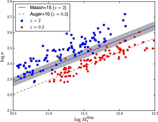
$Velocity dispersion as a function of stellar mass of the ‘M* model’ mock sample (the ‘σ sample’ behaves similarly), at z = 0.2 (red circles) and z = 2 (blue squares). Dashed line: best-fitting $M_{\ast }^{\mathrm{Salp}}\text{--}\sigma$ relation measured by Auger et al. (2010b) on a sample of strong lens early-type galaxies. Blue line: $M_{\ast }^{\mathrm{Salp}}\text{--}\sigma$ relation at z = 2 inferred by Mason et al. (2015). The 68 per cent confidence region is marked by the shaded region.$

Figure 1.

Velocity dispersion as a function of stellar mass of the ‘M_* model’ mock sample (the ‘σ sample’ behaves similarly), at z = 0.2 (red circles) and z = 2 (blue squares). Dashed line: best-fitting |$M_{\ast }^{\mathrm{Salp}}\text{--}\sigma$| relation measured by Auger et al. (2010b) on a sample of strong lens early-type galaxies. Blue line: |$M_{\ast }^{\mathrm{Salp}}\text{--}\sigma$| relation at z = 2 inferred by Mason et al. (2015). The 68 per cent confidence region is marked by the shaded region.

Open in new tab Download slide

Finally, we need to describe the growth in true stellar mass for our centrals, which in turn requires to define the IMF of the accreted satellites. Similarly to the velocity dispersion case, we assign the IMF of satellites using equation (4), where the coefficients are determined at each time-step by fitting the distribution of IMF as a function of stellar mass and velocity dispersion of the centrals.

We do not keep track of the spatial distribution of stars within our galaxies. Although observations could in principle detect spatial variations in IMF within a galaxy (Martín-Navarro et al. 2015a), provided that metallicity gradients are accurately accounted for (McConnell, Lu & Mann 2016), and put interesting constraints on IMF differences between the in situ population and that of the accreted stars that is left for the future work.

3 REFERENCE IMF MEASUREMENTS

The main goal of this work is to make predictions on the distribution of the IMF in massive galaxies as a function of redshift, using low-redshift observations as a reference point. To ensure self-consistency when comparing with results at high redshift, we choose the IMF measurements from Sonnenfeld et al. (2015, hereafter S15) to be such reference point. In this section, we summarize the main results of that work and carry out some additional analysis needed in order to calibrate our models to the observations.

S15 measured the effective stellar IMF for a sample of 80 early-type galaxies using strong lensing in combination with velocity dispersion data to constrain the stellar mass |$M_{\ast }^{\mathrm{true}}$| of each object. Measurements of α_IMF for individual objects are very noisy. To cope with the low signal to noise of individual measurements, S15 combined them with a hierarchical Bayesian inference approach, in which they modelled the distribution of IMF normalization of the population of massive galaxies as a Gaussian and allowed the mean of such Gaussian to be a function of redshift, stellar mass and projected stellar mass density. The analysis yielded the detection of a positive trend between the effective IMF and stellar mass and no detection of a dependence on redshift or stellar mass density.

The S15 analysis did not explore dependences between velocity dispersion and IMF, which we consider in our model. Moreover, the relations between stellar mass and IMF explored by S15 were based on |$M_{\ast }^{\mathrm{true}}$|⁠, instead of |$M_{\ast }^{\mathrm{Salp}}$|⁠. For this reason, we re-analyse here the S15 sample and fit for a dependence of the IMF on |$M_{\ast }^{\mathrm{Salp}}$| and σ, as well as redshift. We then describe the distribution in effective IMF of the S15 sample of galaxies as a Gaussian with mean

\begin{eqnarray} &&{a_z(z - 0.3) + a_{\ast }(\log {M_{\ast }^{\mathrm{Salp}}} - 11.5)}\nonumber\\ &&\qquad\qquad + a_\sigma (\log {\sigma } - 2.4) + \log {\alpha _{\mathrm{IMF},0}} \end{eqnarray}

(11)

and dispersion s. The pivot points z = 0.3, |$\log {M_{\ast }^{\mathrm{Salp}}}=11.5$|⁠, and log σ = 2.4 are very close to the median values of the corresponding quantities in the S15 sample. This allows us to minimize the covariance in the inference of the paramteres a_z, a_*, and a_σ. We fit for a_z, a_*, a_σ, α_{IMF, 0}, and s using a similar hierarchical Bayesian inference method as the one used by S15. Details of the fitting procedure are given in the appendix. The main assumptions of this model are a fixed Navarro Frenk and White (Navarro, Frenk & White 1997, NFW) shape for the dark-matter distribution, a de Vaucouleurs (de Vaucouleurs 1948) profile with spatially constant mass-to-light ratio and isotropic velocity distribution for the stars.

In Fig. 2, we plot the posterior probability distribution for the parameters describing the IMF, marginalized over the other model parameters (which include parameters describing the dark-matter distribution). Consistently with the S15 analysis, we find an average IMF normalization slightly heavier than a Salpeter IMF (log α_{IMF, 0} = 0.06 ± 0.02). There is a strong degeneracy between the parameters a_* and a_σ, meaning that the data can be described either with a dependence of the IMF on stellar mass or on velocity dispersion. This degeneracy is a consequence of the tight correlation between stellar mass and velocity dispersion in early-type galaxies. Nevertheless, the data, under the assumptions specified above and discussed in the appendix, exclude a Universal IMF at the 3σ level and show a trend of increasing IMF normalization with increasing mass and/or velocity dispersion.

Figure 2.

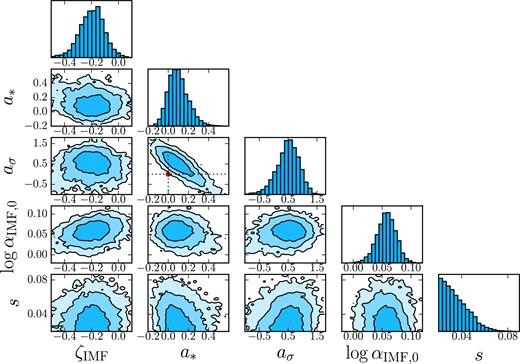
Posterior probability distribution of parameters describing the effective IMF of early-type galaxies, modelled as a Gaussian with mean given by equation (11) and dispersion s and fitted to lensing and stellar kinematics observations of the S15 sample. Different levels represent the 68, 95, and 99.7 per cent enclosed probability regions. The red dot marks the values a_* = 0 and a_σ = 0, corresponding to a Universal IMF.

Open in new tab Download slide

Given that (1) our inference on the parameter a_* is consistent with zero, (2) a description of the galaxy population in which the IMF depends simultaneously on velocity dispersion and stellar mass is not of trivial interpretation, and (3) a large number of works in the literature focus on trends of the IMF with velocity dispersion alone, we repeat the analysis by fixing a_* = 0. In this simpler description of the data, the IMF mismatch parameter is then distributed as a Gaussian with mean given by

\begin{equation} a_z(z - 0.3) + a_\sigma (\log {\sigma } - 2.4) + \log {\alpha _{\mathrm{IMF},0}} \end{equation}

(12)

and dispersion s. The posterior probability distribution of the parameters of this model is plotted in Fig. 3.

Figure 3.

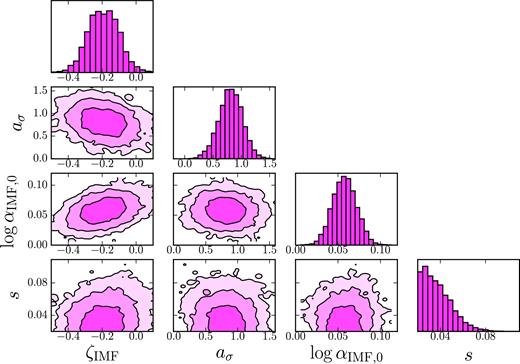
Posterior probability distribution of parameters describing the effective IMF of early-type galaxies, modelled as a Gaussian with mean given by equation (12) and dispersion s and fitted to lensing and stellar kinematics observations of the S15 sample. Different levels represent the 68, 95, and 99.7 per cent enclosed probability regions.

Open in new tab Download slide

4 RESULTS

4.1 Evolution of the α_IMF–|$M_{\ast }^{\mathrm{Salp}}$| and α_IMF–σ relations

We evolved our mock population of galaxies from z = 2 to z = 0.3, the median redshift of the S15 sample and the redshift at which lensing constraints on the IMF are most robust. In Fig. 4, we plot the IMF mismatch parameter for our mock sample of galaxies at three different redshifts (z = 2, z = 1, and z = 0.3), as a function of stellar mass and velocity dispersion, for each model. At each redshift snapshot and for each model we fit for a power-law dependence of the IMF on stellar mass

\begin{equation} \log {\alpha _{\mathrm{IMF}}} = c_{\ast }\left(\log {M_{\ast }^{\mathrm{Salp}}} - 11.5\right) + d_{\ast } \end{equation}

(13)

and velocity dispersion

\begin{equation} \log {\alpha _{\mathrm{IMF}}} = c_\sigma (\log {\sigma } - 2.4) + d_\sigma . \end{equation}

(14)

The best-fitting curves are overplotted in Fig. 4 and values of the parameters are reported in Table 1.

Figure 4.

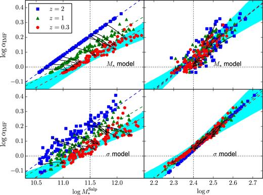
IMF mismatch parameter α_IMF as a function of stellar mass (left-hand panels) and central velocity dispersion (right-hand panels) for the ‘M_* model’ (top panels) and ‘σ model’ (bottom panels) IMF recipes, at z = 2, z = 1, and z = 0.3. Solid lines: evolutionary tracks between z = 2 and z = 0.3 of a few representative galaxies. Dashed lines: fits of equation (13) and equation (14) to the data in each redshift snapshot. Shaded regions: observational constraints from Section 3, obtained using data from S15 at z = 0.3. Horizontal dotted lines: IMF mismatch parameter corresponding to a Salpeter IMF. Vertical dotted lines: pivot point of equation (13) (left-hand panels) and equation (14) (right-hand panels).

Open in new tab Download slide

Table 1.

Open in new tab

The best-fitting parameters of equation (13) and equation (14) to the mock data shown in Fig. 4. The third number in each set represents the residual scatter around the best-fitting relation.

Data set	Equation (13) fit	Equation (14) fit
	(c_, d_, s_*)	(c_σ, d_σ, s_σ)
‘M_* model (z = 2)’	(0.26, 0.21, 0.00)	(1.06, 0.06, 0.06)
‘M_* model (z = 1)’	(0.21, 0.13, 0.02)	(1.06, 0.06, 0.04)
‘M_* model (z = 0.3)’	(0.20, 0.06, 0.02)	(1.08, 0.05, 0.04)
‘σ model (z = 2)’	(0.24, 0.19, 0.05)	(1.20, 0.03, 0.00)
‘σ model (z = 1)’	(0.19, 0.11, 0.04)	(1.06, 0.05, 0.01)
‘σ model (z = 0.3)’	(0.18, 0.05, 0.03)	(1.02, 0.05, 0.01)

Data set	Equation (13) fit	Equation (14) fit
	(c_, d_, s_*)	(c_σ, d_σ, s_σ)
‘M_* model (z = 2)’	(0.26, 0.21, 0.00)	(1.06, 0.06, 0.06)
‘M_* model (z = 1)’	(0.21, 0.13, 0.02)	(1.06, 0.06, 0.04)
‘M_* model (z = 0.3)’	(0.20, 0.06, 0.02)	(1.08, 0.05, 0.04)
‘σ model (z = 2)’	(0.24, 0.19, 0.05)	(1.20, 0.03, 0.00)
‘σ model (z = 1)’	(0.19, 0.11, 0.04)	(1.06, 0.05, 0.01)
‘σ model (z = 0.3)’	(0.18, 0.05, 0.03)	(1.02, 0.05, 0.01)

Table 1.

Open in new tab

The best-fitting parameters of equation (13) and equation (14) to the mock data shown in Fig. 4. The third number in each set represents the residual scatter around the best-fitting relation.

Data set	Equation (13) fit	Equation (14) fit
	(c_, d_, s_*)	(c_σ, d_σ, s_σ)
‘M_* model (z = 2)’	(0.26, 0.21, 0.00)	(1.06, 0.06, 0.06)
‘M_* model (z = 1)’	(0.21, 0.13, 0.02)	(1.06, 0.06, 0.04)
‘M_* model (z = 0.3)’	(0.20, 0.06, 0.02)	(1.08, 0.05, 0.04)
‘σ model (z = 2)’	(0.24, 0.19, 0.05)	(1.20, 0.03, 0.00)
‘σ model (z = 1)’	(0.19, 0.11, 0.04)	(1.06, 0.05, 0.01)
‘σ model (z = 0.3)’	(0.18, 0.05, 0.03)	(1.02, 0.05, 0.01)

Data set	Equation (13) fit	Equation (14) fit
	(c_, d_, s_*)	(c_σ, d_σ, s_σ)
‘M_* model (z = 2)’	(0.26, 0.21, 0.00)	(1.06, 0.06, 0.06)
‘M_* model (z = 1)’	(0.21, 0.13, 0.02)	(1.06, 0.06, 0.04)
‘M_* model (z = 0.3)’	(0.20, 0.06, 0.02)	(1.08, 0.05, 0.04)
‘σ model (z = 2)’	(0.24, 0.19, 0.05)	(1.20, 0.03, 0.00)
‘σ model (z = 1)’	(0.19, 0.11, 0.04)	(1.06, 0.05, 0.01)
‘σ model (z = 0.3)’	(0.18, 0.05, 0.03)	(1.02, 0.05, 0.01)

As can be seen by comparing the left-hand panels of Fig. 4 with the right-hand panels, correlations of the effective IMF with stellar mass correspond to similar correlations with velocity dispersion and vice versa. This is again a consequence of the relatively tight correlation between galaxy stellar mass and velocity dispersion in the mock sample (and in observations; Fig. 1). By looking at the redshift evolution of our mock samples, we can see that the IMF normalization of individual objects decreases with time. This can be easily understood: central galaxies grow by merging with smaller objects which, by construction, have a lighter IMF and therefore bring the effective IMF of the post-merger galaxy towards smaller values. Focusing on the left-hand side of Fig. 4, one can also notice how the most massive galaxies experience the largest decrease in IMF normalization. As a result, the correlation between stellar mass and effective IMF becomes shallower with time (the coefficient c_* in equation 13 decreases with time). The reason for this tilt will be discussed in Section 5. A similar trend is seen for the correlation between σ and α_IMF in the ‘σ model’ (the bottom-right panel of Fig. 4), becoming shallower with time. In contrast, for the ‘M_* model’, the original correlation between velocity dispersion and IMF is roughly preserved by dry mergers.

While the mean trends between stellar mass or velocity dispersion and stellar IMF evolve very similarly for both models examined here, the two models differ in terms of scatter around these correlations. The ‘M_* model’ is initialized with zero scatter around the |$M_{\ast }^{\mathrm{Salp}}\text{--}\alpha _{\mathrm{IMF}}$| relation, but by z = 1 a substantial scatter is introduced. For the ‘σ model’, however, the relation between α_IMF and σ in place at z = 2 remains remarkably tight down to z = 0.3. This is a consequence of the different direction of the evolutionary tracks in |$M_{\ast }^{\mathrm{Salp}}\text{--}\alpha _{\mathrm{IMF}}$| and σ–α_IMF space. Objects evolve roughly perpendicular to the |$M_{\ast }^{\mathrm{Salp}}\text{--}\alpha _{\mathrm{IMF}}$| relation, quickly introducing scatter, while as discussed above the σ–α_IMF relation is mostly preserved due to the coincidence between direction of evolution and correlation in σ–α_IMF space. This prediction depends critically on our model for the evolution of the velocity dispersion with dry mergers, based on the assumption of parabolic orbits for the accreted satellites, which predicts steadily declining values of σ with time for individual galaxies. Dark-matter-only cosmological simulations show that the parabolic orbit approximation tends on average to underestimate the post-merger velocity dispersion (Posti et al. 2014). For instance, in the simple case in which σ remains constant after each merger, objects would move vertically in the σ–α_IMF plane, qualitatively changing the right-hand panels of Fig. 4.

4.2 Evolution of the mock galaxies in the α_IMF–|$M_{\ast }^{\mathrm{Salp}}$|–σ space

Fig. 4 only shows how the parameters |$M_{\ast }^{\mathrm{Salp}}$| and σ correlate individually with the effective IMF. We now examine simultaneous dependences of the IMF on stellar mass and velocity dispersion, that is how α_IMF scales with |$M_{\ast }^{\mathrm{Salp}}$| at fixed σ and vice versa. For each mock sample at each time-step, we determine the average of the logarithm of the stellar mass and velocity dispersion, μ_*(z) and μ_σ(z), then fit equation (4) to the IMF distribution and plot the measured coefficients a_* and a_σ in Fig. 5.

Figure 5.

Coefficients a_* and a_σ, describing the dependence of the effective IMF on stellar mass and velocity dispersion, obtained by fitting equation (4) to mock data generated with the ‘M_* model’ and ‘σ model’ prescriptions at each time-step. The symbols correspond to different redshifts as in Fig. 4. The shaded region marks the observational constraint at z = 0.3 obtained in Section 3 from the S15 data. Different contours mark regions of 68, 95, and 99.7 per cent enclosed probability.

Open in new tab Download slide

The starting (z = 2) point in the a_* − a_σ space is by construction very different for the two mock sets. For the ‘M_* model’, the initial dependence on stellar mass is in part converted into a dependence on velocity dispersion as a result of dry mergers. By contrast, the coefficients describing the σ model at z = 0.3 are very close to the z = 2 values. The initial dependence of the IMF on velocity dispersion becomes slightly weaker, while no significant dependence on stellar mass (at fixed velocity dispersion) is introduced. This is a result of dry mergers preserving the tight correlation between σ and α_IMF, apparent in the bottom-right panel of Fig. 4. As discussed above, this prediction relies in turn on the assumed evolution of the velocity dispersion. If we allow for a milder decline in velocity dispersion with dry mergers, we observe a more significant mixing between stellar mass and velocity dispersion dependence of the IMF, the red dot corresponding to the ‘σ model’ in Fig. 5 approaching the corresponding dot of the ‘M_* model’.

4.3 Average IMF normalization as a function of redshift at fixed velocity dispersion

Finally, we examine how the IMF normalization of the mock sample at fixed galaxy properties evolves in time and compare it with the S15 measurements. In Section 3, we presented two different descriptions of the IMF distribution: one in which α_IMF scales with redshift, stellar mass, and velocity dispersion (equation 11) and a simpler one in which the dependence on stellar mass is ignored (equation 12). Since, as shown in Fig. 5, the S15 data are unable to put interesting constraints on the separate dependence of the IMF on |$M_{\ast }^{\mathrm{Salp}}$| and σ, we adopt the latter description from now on and consider for simplicity only dependences of α_IMF on velocity dispersion and redshift.

In Fig. 6, we plot the mean IMF normalization for galaxies at log σ = 2.4 of the mock populations together with the value measured in the analysis of the S15 data. For the model curves, this is given by parameter d_σ of equation (14), fitted for at each time-step. For the S15 measurements, the observational band is obtained by evaluating equation (12) at log σ = 2.4 at each redshift between z = 0 and z = 0.8 (there are no objects at z > 0.8 in the S15 sample). We see a 2σ discrepancy between both models and the S15 constraints.

Figure 6.

Solid lines: Average effective IMF normalization for galaxies at fixed velocity dispersion log σ = 2.4 of the mock samples, parameter d_σ in equation (14), as a function of redshift. Shaded regions: Observational constraints from the analysis of the S15 data carried out in Section 3, obtained by evaluating equation (12) at log σ = 2.4. Different levels mark the 68, 95, and 99.7 per cent enclosed probability regions. Points with error bars: average IMF normalization at log σ = 2.4 inferred by Conroy & van Dokkum (2012), Spiniello et al. (2014), and Shetty & Cappellari (2014). Horizontal error bars indicate the range in redshift of the galaxies within the samples. Triangles: upper limit estimates of α_IMF from isotropic mass-follows-light spherical Jeans dynamical models applied to velocity dispersion measurements from the literature, corrected to the pivot point assuming the value of a_σ measured in the S15 analysis. The triangle marks the 1–σ (84 percentile) limit.

Open in new tab Download slide

We then compare our models with several sets of measurements from the literature. Conroy & van Dokkum (2012) constrained the IMF of a sample of nearby massive ellipticals by fitting stellar population models to spectral indices sensitive to the abundance of low-mass stars. They found a trend between IMF slope, and normalization, and stellar velocity dispersion. We took their measurements of the IMF normalization, converted them to our definition of α_IMF, then fitted for a power-law dependence between α_IMF and σ and plotted the value inferred at log σ = 2.4 in Fig. 6. Using a similar technique, Spiniello et al. (2014) constrained the IMF of low-redshift early-type galaxies by fitting stellar population models to a large sample of the Sloan Digital Sky Survey spectra. They measured a positive trend between IMF normalization and galaxy velocity dispersion. In Fig. 6, we plot the value of α_IMF inferred by Spiniello et al. (2014) for galaxies at log σ = 2.4.

These are all low-redshift measurements, plotted with the purpose of estimating the systematic uncertainty in the determination of α_IMF with different techniques. At higher redshift, Shetty & Cappellari (2014) constrained the IMF of 68 galaxies at z ∼ 0.75 from dynamical modelling of single aperture stellar kinematics data. Their analysis assumes that the total density profile follows the light distribution, neglecting the contribution of dark matter. Therefore, their results are meant to be an upper limit on the normalization factor α_IMF.

Although Shetty & Cappellari (2014) report values of the IMF normalization and velocity dispersion for each object, we cannot use this information directly to fit for a trend between α_IMF and σ because in dynamical analysis, unlike in the spectral fitting technique, the measurement uncertainty on the velocity dispersion is strongly correlated with that on the IMF. An accurate fit of α_IMF versus σ would then require a full knowledge of the measurement uncertainty in the σ–α_IMF plane, which, unlike for the S15 sample, is not available. We then fix the slope of the σ–α_IMF relation to the value of a_σ measured in the analysis of the S15 data and fit for the normalization of the IMF at log σ = 2.4 in the Shetty & Cappellari (2014) sample. The resulting value of α_IMF is above both the ‘M_* model’ and the ‘σ model’, though this apparent tension is likely to disappear once the contribution from dark matter is taken into account.

At redshift higher than z ∼ 0.8, there are no robust dynamical measurements of the IMF normalization. However, we can put upper limits on the stellar mass, and the IMF, of galaxies with measured velocity dispersion using dynamical arguments. We can write the virial theorem for a stationary stellar system,

\begin{equation} K_V\sigma _{e2}^2 = G\frac{M}{R_e}, \end{equation}

(15)

where M is the total (stellar plus dark-matter) mass, R_e the projected half-light radius, σ_e2 the luminosity-weighted line-of-sight velocity dispersion within a circular aperture of radius R_e/2, and K_V is a coefficient that takes into account the density profile of mass and light, geometrical effects and the distribution of stellar orbits. In the limit in which all the mass is in stars (no dark matter) |$M=M_{\ast }^{\mathrm{true}}$|⁠, so the virial coefficient K_V can be used to put an upper limit on the stellar mass.

We then collect measurements of σ_e2 in the redshift range 0.8 < z < 2 from the literature. Following Mason et al. (2015), we consider measurements from van der Wel et al. (2008), Cappellari et al. (2009), Newman et al. (2010), Onodera et al. (2012), Bezanson et al. (2013), van de Sande et al. (2013), as well as measurements from Gargiulo et al. (2015b). We assume isotropic stellar velocity distribution, consistently with the analysis of the S15 data, and use the spherical Jeans equation to calculate K_V for a mass-follows-light Sérsic (1968)) profile with structural parameters given by the observed values. The adopted values of K_V range from 3.19 (corresponding to a Sérsic index n = 8.0) to 7.18 (corresponding to n = 1.1). We solve for |$M=M_{\ast }^{\mathrm{true}}$| in equation (15) and divide the stellar mass by the value obtained from stellar population synthesis assuming a Salpeter IMF to obtain α_IMF. Finally, we correct these measurements to the pivot point log σ = 2.4 using the values of a_σ measured in the analysis of S15 data. 1σ upper limits (84 per cent enclosed probability) on log α_IMF for individual galaxies are plotted in Fig. 6. 39 per cent (34 per cent) of the objects have 1σ upper limits below the ‘M_* model’ (‘σ model’), indicating tension between both models and observations. Part of this tension could simply be due to intrinsic scatter in the distribution of IMF in the population of galaxies. Although in Section 3 we constrained the intrinsic scatter to be below 0.08 in log α_IMF, there are indications that the scatter in IMF might be larger (Smith & Lucey 2013). Other possible causes for the discrepancy between models and observations are discussed in the next section.

For completeness, we point out that while dynamical measurements appear to indicate an IMF normalization that becomes heavier with time, a spectral study of the IMF of massive galaxies at 0.9 < z < 1.5 by Martín-Navarro et al. (2015b) suggests the opposite: they find a steeper IMF slope (i.e. a more bottom-heavy IMF and therefore a larger value of α_IMF) with respect to measurements carried out at low z with a similar technique (Ferreras et al. 2013). However, converting directly the IMF slopes derived by Martín-Navarro et al. (2015b) into measurements of α_IMF results in values significantly larger than allowed by lensing and dynamics constraints on similar galaxies. Unless the two samples of galaxies are dramatically different in properties, this tension and the fact that the lensing upper limits are hard to circumvent highlight the challenge of converting luminosity weighted measurements to estimate α_IMF at these redshifts.

5 DISCUSSION

5.1 Comparison of models with observations

Our model predicts that the effective IMF α_IMF of massive early-type galaxies, at fixed velocity dispersion, should remain roughly constant with redshift. However, such a trend is not apparent from the few observational constraints on the IMF available at z > 0.3: in fact some data, including the S15 measurements used to calibrate our model at z = 0.3, suggest that α_IMF might be lower at higher z (see also Tortora et al. 2014). A possible source for this tension is the treatment of the dark-matter component in the analysis of the S15 data, in which we fixed the shape of the dark-matter density distribution to an NFW profile (see the appendix). The dark-matter slope is however highly degenerate with the IMF (see e.g. Auger et al. 2010b). In particular, if the dark-matter profile is getting steeper with time the IMF normalization inferred at low redshift would decrease, bringing the model in better agreement with the measurements. However, such a hypothesis is difficult to verify with the current data.

Although the discrepancy between the models and the S15 measurements is within 3σ, a similar tension is seen in the comparison with dynamical estimates on the IMF at z > 1. Dark matter cannot be a source of bias in this case because its contribution is ignored in our treatment of high-redshift measurements.

Another possible source of error that could be affecting the measurements differently at different redshifts is the presence of spatial gradients in the IMF. As shown by Newman, Ellis & Treu (2015), an IMF that becomes less heavy at increasing distance from the centre of a galaxy would bias lensing and dynamical studies that assume a spatially constant IMF (such as the observations presented here) towards a globally heavier IMF. A radial gradient in IMF could be created by dry mergers if the newly accreted material has a more extended distribution than the pre-existing stellar distribution. Indeed, minor dry mergers are predicted to build up an extended envelope of stars (Naab et al. 2009; Hopkins et al. 2010) which, in the context of our model, would have a lighter IMF compared to the central parts. Such an extended envelope of stars with lighter IMF would grow in time, producing a stronger bias towards a heavier inferred IMF in low-redshift galaxies. Such a scenario appears to be supported, indirectly, by the ubiquitous presence of colour gradients in ETGs (van Dokkum et al. 2010), and more directly by spatially resolved spectroscopic studies of the IMF in massive ETGs: Martín-Navarro et al. (2015a) and La Barbera et al. (2016) claimed a detection of a spatial variation of the IMF, heavier in the centre, in three massive early-type galaxies.

Testing whether unaccounted for spatial gradients could be the cause of the apparent evolution in IMF would require a much more complex model than the one explored in this work, and we therefore leave it to future study. We stress out however that while our theoretical model makes predictions on a global quantity integrated over the entirety of a galaxy, namely the effective IMF, such quantity might not be easily recoverable in dynamical measurements like the ones presented in Fig. 6 in case spatial gradients in the IMF are present.

Assuming that the tension between model and data is real and not the result of systematic errors or selection effects, our simple scenario based on dry mergers must be modified. In a previous work, we showed how a very similar dry-merger evolution model to the one presented here is unable to reproduce both the size evolution and the evolution in the slope of the density profile of massive galaxies at z < 1 (Sonnenfeld, Nipoti & Treu 2014). The model predicted density slopes that become shallower with time, at odds with lensing constraints. As a solution, we proposed a scenario in which a small fraction (about 10 per cent) of the accreted baryonic mass is in the form of gas that falls to the centre of the galaxy causing the density profile to steepen and the velocity dispersion to increase as a result of adiabatic contraction.

Such a scenario would modify the predicted IMF evolution in two ways: with the addition of a population of stars formed in situ and by modifying the evolution of the velocity dispersion. Contributing with less than 10 per cent of the final mass, the newly formed stars would not change significantly the effective IMF of a galaxy unless their IMF normalization differs by a factor of a few with respect to that of the accreted satellites, which seems unplausible. However, a central core of stars with a different IMF from the preexisting population would create a radial gradient in the IMF which, as discussed above, could be a source of bias for dynamical measurements. The increase in velocity dispersion caused by the adiabatic contraction from the infall of gas would improve the agreement with the observed evolution of the |$M_{\ast }^{\mathrm{Salp}}\text{--}\sigma$| relation. We have shown in Fig. 1 how our model tends to overpredict the average velocity dispersion at z = 2 with respect to observations, meaning that a slower decline in velocity dispersion is required to precisely match both z = 0 and z = 2 velocity dispersion measurements. However, in a scenario in which the velocity dispersion evolves more slowly the σ–α_IMF correlation will not be preserved, as predicted in our purely dry-merger model (see the right-hand panel of Fig. 4), but will become shallower with time. This means that at fixed σ the IMF will be heavier at larger z, increasing the tension between model and z > 1 data.

Finally, a possible solution to the discrepancy would be to allow for completely different IMF distributions between centrals and satellites. Our model assumes that the scaling relation between the effective IMF of accreted galaxies and their galaxy properties is the same as that of centrals, extrapolated to low masses. If we allow, for instance, the IMF normalization of satellites to be on average heavier than that of centrals, individual galaxies would evolve towards a heavier effective IMF with time, in the direction suggested by the data. There are currently no robust observations through which we can test this hypothesis.

5.2 IMF evolution and average merger mass ratio

A second prediction of our model is that the decrease of the IMF mismatch parameter with time is stronger for the more massive objects. This is shown by the evolution in the tilt of the |$\alpha _{\mathrm{IMF}}\text{--}M_{\ast }^{\mathrm{Salp}}$| correlation with redshift seen in the left-hand column of Fig. 4. To understand the origin of this effect, in Fig. 7, we plot the fractional change in effective IMF between z = 2 and z = 0, Δlog α_IMF = log α_IMF(z = 0) − log α_IMF(z = 2) of our mock galaxies together with key quantities such as the initial halo mass and initial stellar mass and accreted stellar mass. The effective IMF of individual galaxies in our sample generally decreases with time (Δlog α_IMF < 0). This is easily understood, as by definition central galaxies merge with less massive systems that, in our model, have a lighter IMF. In order to produce a dependence of the IMF on mass that becomes shallower with time it is necessary for the more massive systems to have a stronger decrease in their IMF with time (more negative values of Δlog α_IMF). As can be seen in the bottom-left panel of Fig. 7, this is indeed the case.

$Distribution in stellar mass $M_{\ast }^{\mathrm{Salp}}$ and halo mass Mh at z = 2, fractional variation in stellar mass $\Delta \log {M_{\ast }^{\mathrm{Salp}}}$ and effective IMF Δlog αIMF between z = 0 and z = 2, and stellar mass-weighted merger mass ratio 〈ξ〉*, as defined in equation (16). Purple dots: ‘M* model’. Green dots: ‘σ model’.$

Figure 7.

Distribution in stellar mass |$M_{\ast }^{\mathrm{Salp}}$| and halo mass M_h at z = 2, fractional variation in stellar mass |$\Delta \log {M_{\ast }^{\mathrm{Salp}}}$| and effective IMF Δlog α_IMF between z = 0 and z = 2, and stellar mass-weighted merger mass ratio 〈ξ〉_*, as defined in equation (16). Purple dots: ‘M_* model’. Green dots: ‘σ model’.

Open in new tab Download slide

Differences in Δlog α_IMF reflect differences in merger history. Since mergers tend to decrease the effective IMF normalization, we expect galaxies with the highest increase in stellar mass to also show the largest changes in effective IMF. However, this is not observed to be the case, as can be seen from Fig. 7 (fourth row, third column). If the amount of accretion does not play a central role in setting the final IMF, then the different change in IMF between low-mass and high-mass systems must be set by differences in the type of mergers. To quantify this, we measure the accreted stellar mass-weighted merger mass ratio, 〈ξ〉_*, defined as the average over all mergers between z = 2 and z = 0 of the mass ratio between the accreted satellites and the central halo weighted by the accreted stellar mass with each merger:

\begin{equation} \!\left\langle \xi \right\rangle _{\ast } = \frac{\int \text{d}z \int \text{d}\xi \xi f(\xi , z)}{\int \text{d}z \int \text{d}\xi f(\xi , z)}, \end{equation}

(16)

with

\begin{equation} f(\xi , z) \equiv \frac{\mathrm{d}^2N_{\mathrm{merg}}}{\mathrm{d}z \mathrm{d}\xi } \mathcal {R}_{{\ast },h}(\xi M_{\mathrm{h}}, z)\xi M_{\mathrm{h}}. \end{equation}

(17)

〈ξ〉_* is plotted in Fig. 7. We see that 〈ξ〉_* increases for decreasing halo and stellar mass. This means that for the most massive galaxies, the bulk of the accreted stellar mass is brought in through mergers of relatively small mass ratio, while for less massive galaxies major mergers play a more important role. Given our IMF prescription, where the heaviness of the IMF of satellites increases with mass, minor mergers produce a stronger decrease in the effective IMF of a galaxy than major mergers at fixed accreted stellar mass. This is seen in the bottom-right panel of Fig. 7, where 〈ξ〉_* correlates with the change in effective IMF. We then conclude that the shallowing of the |$M_{\ast }^{\mathrm{Salp}}\text{--}\alpha _{\mathrm{IMF}}$| or σ–α_IMF trends with time seen in our Fig. 4 is a result of the different relative importance of major and minor mergers in systems of different mass.

5.3 Dependence of the IMF on global galaxy properties

Another prediction of our model is the mixing between stellar mass and velocity dispersion dependence of the IMF shown in Fig. 5. The dependence of velocity dispersion, a_σ, seen at z = 0 in the ‘M_* model’ can be easily understood. The ‘M_* model’ is initialized with zero scatter around the |$M_{\ast }^{\mathrm{Salp}}\text{--}\alpha _{\mathrm{IMF}}$| relation at z = 2. Since then, individual galaxies evolve roughly perpendicularly to the |$M_{\ast }^{\mathrm{Salp}}\text{--}\alpha _{\mathrm{IMF}}$| relation (the left-hand panels of Fig. 4), so that by z = 1 a significant scatter is introduced. At that point, a pure dependence of the IMF on stellar mass is no longer a good description of the model, and a mixed dependence on both M_* and σ is preferred. In contrast in the ‘σ model’ galaxies evolve parallel to the σ–α_IMF relation in place at z = 2 and very little scatter is added down to z = 0.3, so that measuring the scatter in IMF as a function of z is potentially a powerful diagnostic. No additional dependence on M_* is required to describe the data, hence the very small change in the parameters a_* and a_σ for this model. As discussed in Section 4 however, this prediction relies on the assumption of parabolic orbits for the accreted satellites. If we allow for a milder decrease in velocity dispersion with dry mergers, we find a larger increase in the parameter a_* and a correspondingly larger decrease in a_σ for the ‘σ model’. Because of the relatively rapid change in the coefficients a_* and a_σ with time, it is very difficult to determine from z ∼ 0 observations which quantity between σ and M_* is the IMF fundamentally dependent on. Current constraints from lensing and stellar dynamics are unable to differentiate between the two models (see Fig. 5).

An important assumption in our model is that all of the growth in stellar mass between z = 2 and z = 0 is due to dry mergers. In other terms, our model only applies to the population of quiescent galaxies at z = 2. This assumption complicates the comparison between predictions from our model and observations, because the number density of quiescent galaxies is observed to increase substantially with time, in particular at z > 1 (e.g. Cassata et al. 2013; Ilbert et al. 2013). Depending on what the IMF of the newly quenched object is, some results might change as a result of the so-called progenitor bias. However, predictions on the z < 1 evolution for the high-mass end of the galaxy distribution should still hold, since the number density of quiescent galaxies shows little evolution in that region of the parameter space (López-Sanjuan et al. 2012).

6 CONCLUSIONS

Using empirically motivated recipes for describing the IMF of massive galaxies together with the dry-merger evolution model developed by Nipoti et al. (2012), we studied the time evolution of the effective IMF, defined as the ratio between the true stellar mass and the stellar mass one would infer assuming a Salpeter IMF, of a population of massive galaxies from z = 2 to z = 0. The models are set up to match the observed correlations between IMF and stellar mass and velocity dispersion in massive early-type galaxies at z ∼ 0.3.

Our model predicts a decrease in the effective IMF of individual objects with time as galaxies merge with systems with a lighter IMF. This is seen in the evolutionary tracks in Fig. 4. Trends between stellar mass and velocity dispersion are qualitatively preserved by dry mergers, but the slope of the correlation between stellar mass and effective IMF becomes less steep with time.

At fixed velocity dispersion, the population of galaxies evolves with a constant or increasing IMF normalization at increasing z. This prediction appears to be in slight tension with the few observational constraints on the IMF available at z > 0.3. However, there are systematic effects that could be affecting observations the importance of which has not fully been assessed yet, most importantly the contribution of dark matter and radial gradients in the IMF. Assuming that the tension is real and not the effect of systematics, the most plausible way to reconcile model and observations is to allow the effective IMF of satellite galaxies to be drawn from a different distribution, heavier at fixed galaxy properties, than that describing centrals.

Finally, we find that the relative dependence of the IMF on stellar mass and velocity dispersion gets mixed by dry mergers, making it difficult to observationally determine the fundamental parameter(s) governing the IMF from z ∼ 0 measurements.

Acknowledgments

CN acknowledges financial support from PRIN MIUR 2010-2011, project ‘The Chemical and Dynamical Evolution of the Milky Way and Local Group Galaxies’, prot. 2010LY5N2T. We thank the anonymous referee for a constructive report that helped improve the paper.

1

The virial velocity dispersion σ_v of a system of total mass M and total kinetic energy K is defined by |$K=(1/2)M\sigma _v^2$|

REFERENCES

Auger

M. W.

,

Treu

T.

,

Gavazzi

R.

,

Bolton

A. S.

,

Koopmans

L. V. E.

,

Marshall

P. J.

,

2010a

,

ApJ

,

721

,

L163

Crossref

Search ADS

Auger

M. W.

,

Treu

T.

,

Bolton

A. S.

,

Gavazzi

R.

,

Koopmans

L. V. E.

,

Marshall

P. J.

,

Moustakas

L. A.

,

Burles

S.

,

2010b

,

ApJ

,

724

,

511

Crossref

Search ADS

Barnabè

M.

,

Czoske

O.

,

Koopmans

L. V. E.

,

Treu

T.

,

Bolton

A. S.

,

2011

,

MNRAS

,

415

,

2215

Crossref

Search ADS

Bastian

N.

,

Covey

K. R.

,

Meyer

M. R.

,

2010

,

ARA&A

,

48

,

339

Crossref

Search ADS

Bekki

K.

,

2013

,

MNRAS

,

436

,

2254

Crossref

Search ADS

Bezanson

R.

,

van Dokkum

P.

,

van de Sande

J.

,

Franx

M.

,

Kriek

M.

,

2013

,

ApJ

,

764

,

L8

Crossref

Search ADS

Boylan-Kolchin

M.

,

Ma

C.-P.

,

Quataert

E.

,

2008

,

MNRAS

,

383

,

93

Crossref

Search ADS

Cappellari

M.

et al. ,

2009

,

ApJ

,

704

,

L34

Crossref

Search ADS

Cappellari

M.

et al. ,

2012

,

Nature

,

484

,

485

Crossref

Search ADS

PubMed

Cassata

P.

et al. ,

2013

,

ApJ

,

775

,

106

Crossref

Search ADS

Chattopadhyay

T.

,

De

T.

,

Warlu

B.

,

Chattopadhyay

A. K.

,

2015

,

ApJ

,

808

,

24

Crossref

Search ADS

Conroy

C.

,

van Dokkum

P. G.

,

2012

,

ApJ

,

760

,

71

Crossref

Search ADS

de Vaucouleurs

G.

,

1948

,

Ann. Astrophys.

,

11

,

247

Dutton

A. A.

,

Mendel

J. T.

,

Simard

L.

,

2012

,

MNRAS

,

422

,

33

Crossref

Search ADS

Fakhouri

O.

,

Ma

C.-P.

,

Boylan-Kolchin

M.

,

2010

,

MNRAS

,

406

,

2267

Crossref

Search ADS

Ferreras

I.

,

La Barbera

F.

,

de la Rosa

I. G.

,

Vazdekis

A.

,

de Carvalho

R. R.

,

Falcón-Barroso

J.

,

Ricciardelli

E.

,

2013

,

MNRAS

,

429

,

L15

Crossref

Search ADS

Ferreras

I.

et al. ,

2014

,

MNRAS

,

444

,

906

Crossref

Search ADS

Fontanot

F.

,

De Lucia

G.

,

Hirschmann

M.

,

Bruzual

G.

,

Charlot

S.

,

Zibetti

S.

,

2016

,

preprint (arXiv:1606.01908)

Gargiulo

I. D.

et al. ,

2015a

,

MNRAS

,

446

,

3820

Crossref

Search ADS

Gargiulo

A.

,

Saracco

P.

,

Longhetti

M.

,

Tamburri

S.

,

Lonoce

I.

,

Ciocca

F.

,

2015b

,

A&A

,

573

,

A110

Crossref

Search ADS

Gavazzi

R.

,

Treu

T.

,

Rhodes

J. D.

,

Koopmans

L. V. E.

,

Bolton

A. S.

,

Burles

S.

,

Massey

R. J.

,

Moustakas

L. A.

,

2007

,

ApJ

,

667

,

176

Crossref

Search ADS

Guszejnov

D.

,

Krumholz

M. R.

,

Hopkins

P. F.

,

2016

,

MNRAS

,

458

,

673

Crossref

Search ADS

Hennebelle

P.

,

Chabrier

G.

,

2011

,

ApJ

,

743

,

L29

Crossref

Search ADS

Hopkins

P. F.

,

2012

,

MNRAS

,

423

,

2037

Crossref

Search ADS

Hopkins

P. F.

,

Bundy

K.

,

Hernquist

L.

,

Wuyts

S.

,

Cox

T. J.

,

2010

,

MNRAS

,

401

,

1099

Crossref

Search ADS

Ilbert

O.

et al. ,

2013

,

A&A

,

556

,

A55

Crossref

Search ADS

Krumholz

M. R.

,

2011

,

ApJ

,

743

,

110

Crossref

Search ADS

La Barbera

F.

,

Ferreras

I.

,

Vazdekis

A.

,

de la Rosa

I. G.

,

de Carvalho

R. R.

,

Trevisan

M.

,

Falcón-Barroso

J.

,

Ricciardelli

E.

,

2013

,

MNRAS

,

433

,

3017

Crossref

Search ADS

La Barbera

F.

,

Vazdekis

A.

,

Ferreras

I.

,

Pasquali

A.

,

Cappellari

M.

,

Martín-Navarro

I.

,

Schönebeck

F.

,

Falcón-Barroso

J.

,

2016

,

MNRAS

,

457

,

1468

Crossref

Search ADS

Leauthaud

A.

et al. ,

2012

,

ApJ

,

744

,

159

Crossref

Search ADS

López-Sanjuan

C.

et al. ,

2012

,

A&A

,

548

,

A7

Crossref

Search ADS

McConnell

N. J.

,

Lu

J. R.

,

Mann

A. W.

,

2016

,

ApJ

,

821

,

39

Crossref

Search ADS

Martín-Navarro

I.

,

La Barbera

F.

,

Vazdekis

A.

,

Falcón-Barroso

J.

,

Ferreras

I.

,

2015a

,

MNRAS

,

447

,

1033

Crossref

Search ADS

Martín-Navarro

I.

et al. ,

2015b

,

ApJ

,

798

,

L4

Crossref

Search ADS

Mason

C. A.

et al. ,

2015

,

ApJ

,

805

,

79

Crossref

Search ADS

Muzzin

A.

et al. ,

2013

,

ApJ

,

777

,

18

Crossref

Search ADS

Naab

T.

,

Johansson

P. H.

,

Ostriker

J. P.

,

2009

,

ApJ

,

699

,

L178

Crossref

Search ADS

Nagashima

M.

,

Lacey

C. G.

,

Okamoto

T.

,

Baugh

C. M.

,

Frenk

C. S.

,

Cole

S.

,

2005

,

MNRAS

,

363

,

L31

Crossref

Search ADS

Navarro

J. F.

,

Frenk

C. S.

,

White

S. D. M.

,

1997

,

ApJ

,

490

,

493

Crossref

Search ADS

Newman

A. B.

,

Ellis

R. S.

,

Treu

T.

,

Bundy

K.

,

2010

,

ApJ

,

717

,

L103

Crossref

Search ADS

Newman

A. B.

,

Treu

T.

,

Ellis

R. S.

,

Sand

D. J.

,

2013

,

ApJ

,

765

,

25

Crossref

Search ADS

Newman

A. B.

,

Ellis

R. S.

,

Treu

T.

,

2015

,

ApJ

,

814

,

26

Crossref

Search ADS

Nipoti

C.

,

Treu

T.

,

Leauthaud

A.

,

Bundy

K.

,

Newman

A. B.

,

Auger

M. W.

,

2012

,

MNRAS

,

422

,

1714

Crossref

Search ADS

Offner

S. S. R.

,

2015

,

preprint (arXiv:1510.06027)

Onodera

M.

et al. ,

2012

,

ApJ

,

755

,

26

Crossref

Search ADS

Posacki

S.

,

Cappellari

M.

,

Treu

T.

,

Pellegrini

S.

,

Ciotti

L.

,

2015

,

MNRAS

,

446

,

493

Crossref

Search ADS

Posti

L.

,

Nipoti

C.

,

Stiavelli

M.

,

Ciotti

L.

,

2014

,

MNRAS

,

440

,

610

Crossref

Search ADS

Ruiz

P.

,

Trujillo

I.

,

Mármol-Queraltó

E.

,

2014

,

MNRAS

,

442

,

347

Crossref

Search ADS

Salpeter

E. E.

,

1955

,

ApJ

,

121

,

161

Crossref

Search ADS

Schneider

M. D.

,

Hogg

D. W.

,

Marshall

P. J.

,

Dawson

W. A.

,

Meyers

J.

,

Bard

D. J.

,

Lang

D.

,

2015

,

ApJ

,

807

,

87

Crossref

Search ADS

Sersic

J. L.

,

1968

, Atlas de Galaxias Australes. Observatorio Astronomico, Cordoba, Argentina

Shetty

S.

,

Cappellari

M.

,

2014

,

ApJ

,

786

,

L10

Crossref

Search ADS

Smith

R. J.

,

Lucey

J. R.

,

2013

,

MNRAS

,

434

,

1964

Crossref

Search ADS

Smith

R. J.

,

Lucey

J. R.

,

Conroy

C.

,

2015

,

MNRAS

,

449

,

3441

Crossref

Search ADS

Sonnenfeld

A.

,

Nipoti

C.

,

Treu

T.

,

2014

,

ApJ

,

786

,

89

Crossref

Search ADS

Sonnenfeld

A.

,

Treu

T.

,

Marshall

P. J.

,

Suyu

S. H.

,

Gavazzi

R.

,

Auger

M. W.

,

Nipoti

C.

,

2015

,

ApJ

,

800

,

94

(S15)

Crossref

Search ADS

Spiniello

C.

,

Trager

S.

,

Koopmans

L. V. E.

,

Conroy

C.

,

2014

,

MNRAS

,

438

,

1483

Crossref

Search ADS

Spiniello

C.

,

Barnabè

M.

,

Koopmans

L. V. E.

,

Trager

S. C.

,

2015

,

MNRAS

,

452

,

L21

Crossref

Search ADS

Tinker

J.

,

Kravtsov

A. V.

,

Klypin

A.

,

Abazajian

K.

,

Warren

M.

,

Yepes

G.

,

Gottlöber

S.

,

Holz

D. E.

,

2008

,

ApJ

,

688

,

709

Crossref

Search ADS

Tortora

C.

,

Romanowsky

A. J.

,

Napolitano

N. R.

,

2013

,

ApJ

,

765

,

8

Crossref

Search ADS

Tortora

C.

,

Napolitano

N. R.

,

Saglia

R. P.

,

Romanowsky

A. J.

,

Covone

G.

,

Capaccioli

M.

,

2014

,

MNRAS

,

445

,

162

Crossref

Search ADS

Treu

T.

,

Auger

M. W.

,

Koopmans

L. V. E.

,

Gavazzi

R.

,

Marshall

P. J.

,

Bolton

A. S.

,

2010

,

ApJ

,

709

,

1195

Crossref

Search ADS

van de Sande

J.

et al. ,

2013

,

ApJ

,

771

,

85

Crossref

Search ADS

van der Wel

A.

,

Holden

B. P.

,

Zirm

A. W.

,

Franx

M.

,

Rettura

A.

,

Illingworth

G. D.

,

Ford

H. C.

,

2008

,

ApJ

,

688

,

48

Crossref

Search ADS

van Dokkum

P. G.

et al. ,

2010

,

ApJ

,

709

,

1018

Crossref

Search ADS

APPENDIX: HIERARCHICAL BAYESIAN INFERENCE

We use a similar hierarchical Bayesian inference method as the one used by S15 to fit for the distribution in IMF of the same sample of galaxies. The method can be summarized as follows. We assume that the density profile of early-type galaxies can be described by the sum of a stellar component with a de Vaucouleurs profile and a dark-matter component with an NFW (Navarro et al. 1997) profile. We parametrize this model in terms of the Salpeter stellar mass |$M_{\ast }^{\mathrm{Salp}}$|⁠, effective radius R_eff, projected dark-matter mass within a cylinder of radius 5 kpc M_{DM, 5}, dark-matter scale radius r_s, and effective IMF α_IMF. Following S15, we assume that the effective radius is known exactly and we fix r_s = 10 R_eff for simplicity. The exact value of r_s has little impact on lensing and dynamics measurements, more sensitive to the mass distribution at the scale of a few kpc, much smaller than typical values of r_s predicted by numerical simulations. The free parameters of each object are then |$M_{\ast }^{\mathrm{Salp}}$|⁠, M_{DM, 5} and α_IMF. For a more compact notation, we label this triplet |$\boldsymbol {\omega }$|⁠:

\begin{equation} \boldsymbol {\omega }\equiv \left(M_{\ast }^{\mathrm{Salp}}, M_{\mathrm{DM},5}, \alpha _{\mathrm{IMF}}\right). \end{equation}

(A1)

From these parameters, we calculate the model central velocity dispersion, σ_e2, using the spherical Jeans equation and assuming isotropic stellar velocity distribution. Though a simplification, the spherical isotropic model has been shown to match results obtained with a more accurate dynamical modelling (Barnabè et al. 2011).

We assume that the parameters of each galaxy are drawn from a distribution for the population of galaxies, described by a set of hyper-parameters|$\boldsymbol {\eta }$|⁠:

\begin{equation} \boldsymbol {\omega }_i\sim {\rm Pr}(\boldsymbol {\omega }_i| \boldsymbol {\eta }), \end{equation}

(A2)

where the subscript i indicates the ith galaxy in the sample. We model this distribution as the product of four terms:

\begin{equation} {\rm Pr}(\boldsymbol {\omega }_i| \boldsymbol {\eta }) = \mathcal {G}_{\ast }\left(M_{{\ast },i}^{\mathrm{Salp}}|\boldsymbol {\eta }\right) \mathcal {G}_\sigma \left(\sigma _{e2,i}|M_{\ast }^{\mathrm{Salp}}, \boldsymbol {\eta }\right) \mathcal {G}_{\mathrm{DM}}\left(M_{\mathrm{DM},5,i}|M_{\ast }^{\mathrm{Salp}},\sigma _{e2,i},\boldsymbol {\eta }\right) \mathcal {G}_{\mathrm{IMF}}\left(\alpha _{\mathrm{IMF},i}|M_{\ast }^{\mathrm{Salp}},\sigma _{e2,i},\boldsymbol {\eta }\right), \end{equation}

(A3)

where each term is a lognormal distribution, respectively, in |$M_{\ast }^{\mathrm{Salp}}$|⁠, σ_e2 (which is a well-defined function of |$\boldsymbol {\omega }$|⁠), M_{DM, 5}, and α_IMF. More precisely,

\begin{equation} \mathcal {G}_{\ast }\left(M_{{\ast },i}^{\mathrm{Salp}}|\boldsymbol {\eta }\right) = \frac{1}{\sqrt{2\pi }\sigma _{\ast }}\exp {\left\lbrace -\frac{\left(\log {M_{{\ast },i}^{\mathrm{Salp}}} - \mu _{\ast }\right)^2}{2\sigma _{\ast }^2}\right\rbrace }. \end{equation}

(A4)

\begin{equation} \mathcal {G}_{\sigma }(\sigma _{e2,i}|\boldsymbol {\eta }) = \frac{1}{\sqrt{2\pi }\sigma _\sigma }\exp {\left\lbrace -\frac{\left(\log {\sigma _{e2,i}} - \mu _\sigma \left(z_i, M_{{\ast },i}^{\mathrm{Salp}}\right)\right)^2}{2\sigma _\sigma ^2}\right\rbrace }, \end{equation}

(A5)

where

\begin{equation} \mu _\sigma \left(M_{{\ast },i}^{\mathrm{Salp}}\right) = \mu _{\sigma ,0} + \zeta _\sigma (z_i - 0.3) + \beta _\sigma \left(\log {M_{{\ast },i}^{\mathrm{Salp}}} - 11.5\right). \end{equation}

(A6)

\begin{equation} \mathcal {G}_{\rm DM }(M_{\mathrm{DM},5,i}|\boldsymbol {\eta }) = \frac{1}{\sqrt{2\pi }\sigma _{\mathrm{DM}}}\exp {\left\lbrace -\frac{\left(\log {M_{\mathrm{DM},5,i}} - \mu _{\mathrm{DM}}\left(z_i, M_{{\ast },i}^{\mathrm{Salp}}, \sigma _{e2,i}\right)\right)^2}{2\sigma _{\mathrm{DM}}^2}\right\rbrace }, \end{equation}

(A7)

where

\begin{equation} \mu _{\mathrm{DM}}\left(M_{{\ast },i}^{\mathrm{Salp}}, \sigma _{e2,i}\right) = \mu _{\mathrm{DM},0} + \zeta _{\mathrm{DM}}(z_i - 0.3) + \beta _{\mathrm{DM}}\left(\log {M_{{\ast },i}^{\mathrm{Salp}}} - 11.5\right) + \xi _{\mathrm{DM}}(\log {\sigma _{e2,i}} - 2.4). \end{equation}

(A8)

\begin{equation} \mathcal {G}_{\rm IMF }\left(\alpha _{\mathrm{IMF},i}|\boldsymbol {\eta }\right) = \frac{1}{\sqrt{2\pi }\sigma _{\mathrm{IMF}}}\exp {\left\lbrace -\frac{\left(\log {\alpha _{\mathrm{IMF},i}} - \mu _{\mathrm{IMF}}\left(z, M_{{\ast },i}^{\mathrm{Salp}}, \sigma _{e2,i}\right)\right)^2}{2\sigma _{\mathrm{IMF}}^2}\right\rbrace }, \end{equation}

(A9)

where

\begin{equation} \mu _{\mathrm{IMF}}\left(M_{{\ast },i}^{\mathrm{Salp}}, \sigma _{e2,i}\right) = a_z(z_i - 0.3) + a_{\ast }\left(\log {M_{{\ast },i}^{\mathrm{Salp}}} - 11.5\right) + a_\sigma (\log {\sigma _{e2,i}} - 2.4) + \log {\alpha _{\mathrm{IMF},0}}. \end{equation}

(A10)

Since the lenses in the S15 study are collected from two different surveys, SLACS and SL2S, we allow for different values in the mean and dispersion of the stellar mass distribution in equation (A4): |$\mu _{\ast }^{\mathrm{SLACS}}$|⁠, |$\mu _{\ast }^{\mathrm{SL2S}}$|⁠, |$\sigma _{\ast }^{\mathrm{SLACS}}$|⁠, and |$\sigma _{\ast }^{\mathrm{SL2S}}$|⁠.

In summary, the distribution of the parameters describing individual galaxies, equation (A3), is described by 18 hyper-parameters:

\begin{equation} \boldsymbol {\eta }= \left\lbrace \mu _{\ast }^{\mathrm{SLACS}}, \mu _{\ast }^{\mathrm{SL2S}}, \sigma _{\ast }^{\mathrm{SLACS}}, \sigma _{\ast }^{\mathrm{SL2S}}, \mu _{\sigma ,0}, \zeta _\sigma , \beta _\sigma , \sigma _\sigma , \mu _{\mathrm{DM}, 0}, \zeta _{\mathrm{DM}}, \beta _{\mathrm{DM}}, \xi _{\mathrm{DM}}, \sigma _{\mathrm{DM}}, \log {\alpha _{\mathrm{IMF}, 0}}, a_z, a_{\ast }, a_\sigma , \sigma _{\mathrm{IMF}} \right\rbrace . \end{equation}

(A11)

We wish to infer the posterior probability distribution of these hyper-parameters given the data |$\boldsymbol {d}$|⁠. The data consist of a measurement of the Einstein radius, velocity dispersion, and stellar mass from stellar population synthesis analysis for each object. From Bayes theorem,

\begin{equation} {\rm Pr}(\boldsymbol {\eta }|\boldsymbol {d}) \propto {\rm Pr}(\boldsymbol {\eta }){\rm Pr}(\boldsymbol {d}|\boldsymbol {\eta }), \end{equation}

(A12)

where |${\rm Pr}(\boldsymbol {\eta })$| is the prior on the hyper-parameters and |${\rm Pr}(\boldsymbol {d}|\boldsymbol {\eta })$| the likelihood of observing the data given the values of the hyper-parameters. This latter term is the product over all galaxies

\begin{equation} {\rm Pr}(\boldsymbol {d}|\boldsymbol {\eta }) = \prod _i {\rm Pr}(\boldsymbol {d}_i|\boldsymbol {\eta }). \end{equation}

(A13)

Each term in this product can in turn be expanded as

\begin{equation} {\rm Pr}(\boldsymbol {d}_i|\boldsymbol {\eta }) = \int d\boldsymbol {\omega }_i{\rm Pr}(\boldsymbol {d}_i|\boldsymbol {\omega }_i) {\rm Pr}(\boldsymbol {\omega }_i|\boldsymbol {\eta }). \end{equation}

(A14)

We assume flat priors on all hyper-parameters. We then sample the posterior probability distribution with a Markov Chain Monte Carlo. The integrals in equation (A14) are evaluated via importance sampling and Monte Carlo integration following Schneider et al. (2015). The inferred values of the hyper-parameters with 1σ uncertainties are reported in Table A1.

Table A1.

Open in new tab

Full model, corresponding to Fig. 2. Median and 68 per cent limits on the posterior probability function of each hyper-parameter, marginalized over the other parameters.

		Parameter description
\|$\mu _{\ast }^{\mathrm{SLACS}}$\|	11.58 ± 0.03	Mean \|$\log {M_{\ast }^{\mathrm{Salp}}}$\|⁠, SLACS sample
\|$\sigma _{\ast }^{\mathrm{SLACS}}$\|	0.19 ± 0.02	Scatter in \|$\log {M_{\ast }^{\mathrm{Salp}}}$\|⁠, SLACS sample
\|$\mu _{\ast }^{\mathrm{SL2S}}$\|	11.50 ± 0.05	Mean \|$\log {M_{\ast }^{\mathrm{Salp}}}$\|⁠, SL2S sample
\|$\sigma _{\ast }^{\mathrm{SL2S}}$\|	0.23 ± 0.04	Scatter in \|$\log {M_{\ast }^{\mathrm{Salp}}}$\|⁠, SL2S sample
μ_{σ, 0}	2.39 ± 0.01	Mean log σ at z = 0.3 and \|$\log {M_{\ast }^{\mathrm{Salp}}}=11.5$\|
ζ_σ	−0.01 ± 0.03	Linear dependence of log σ on z
β_σ	0.19 ± 0.03	Linear dependence of log σ on \|$\log {M_{\ast }^{\mathrm{Salp}}}$\|
σ_σ	0.04 ± 0.01	Scatter in log σ
μ_{DM, 0}	10.60 ± 0.09	Mean log M_{DM, 5} at z = 0.3, \|$\log {M_{\ast }^{\mathrm{Salp}}}=11.5$\| and log σ = 2.4
ζ_DM	1.13 ± 0.27	Linear dependence of log M_{DM, 5} on z
β_DM	0.13 ± 0.25	Linear dependence of log M_{DM, 5} on \|$\log {M_{\ast }^{\mathrm{Salp}}}$\|
ξ_DM	−0.77 ± 0.72	Linear dependence of log M_{DM, 5} on log σ
σ_DM	0.25 ± 0.05	Scatter in log M_{DM, 5}
log α_{IMF, 0}	0.06 ± 0.02	Mean log α_IMF at z = 0.3, \|$\log {M_{\ast }^{\mathrm{Salp}}}=11.5$\| and log σ = 2.4
a_z	−0.20 ± 0.09	Linear dependence of log α_IMF on z
a_*	0.10 ± 0.10	Linear dependence of log α_IMF on \|$\log {M_{\ast }^{\mathrm{Salp}}}$\|
a_σ	0.49 ± 0.39	Linear dependence of log α_IMF on log σ
σ_IMF	0.03 ± 0.01	Scatter in log α_IMF

		Parameter description
\|$\mu _{\ast }^{\mathrm{SLACS}}$\|	11.58 ± 0.03	Mean \|$\log {M_{\ast }^{\mathrm{Salp}}}$\|⁠, SLACS sample
\|$\sigma _{\ast }^{\mathrm{SLACS}}$\|	0.19 ± 0.02	Scatter in \|$\log {M_{\ast }^{\mathrm{Salp}}}$\|⁠, SLACS sample
\|$\mu _{\ast }^{\mathrm{SL2S}}$\|	11.50 ± 0.05	Mean \|$\log {M_{\ast }^{\mathrm{Salp}}}$\|⁠, SL2S sample
\|$\sigma _{\ast }^{\mathrm{SL2S}}$\|	0.23 ± 0.04	Scatter in \|$\log {M_{\ast }^{\mathrm{Salp}}}$\|⁠, SL2S sample
μ_{σ, 0}	2.39 ± 0.01	Mean log σ at z = 0.3 and \|$\log {M_{\ast }^{\mathrm{Salp}}}=11.5$\|
ζ_σ	−0.01 ± 0.03	Linear dependence of log σ on z
β_σ	0.19 ± 0.03	Linear dependence of log σ on \|$\log {M_{\ast }^{\mathrm{Salp}}}$\|
σ_σ	0.04 ± 0.01	Scatter in log σ
μ_{DM, 0}	10.60 ± 0.09	Mean log M_{DM, 5} at z = 0.3, \|$\log {M_{\ast }^{\mathrm{Salp}}}=11.5$\| and log σ = 2.4
ζ_DM	1.13 ± 0.27	Linear dependence of log M_{DM, 5} on z
β_DM	0.13 ± 0.25	Linear dependence of log M_{DM, 5} on \|$\log {M_{\ast }^{\mathrm{Salp}}}$\|
ξ_DM	−0.77 ± 0.72	Linear dependence of log M_{DM, 5} on log σ
σ_DM	0.25 ± 0.05	Scatter in log M_{DM, 5}
log α_{IMF, 0}	0.06 ± 0.02	Mean log α_IMF at z = 0.3, \|$\log {M_{\ast }^{\mathrm{Salp}}}=11.5$\| and log σ = 2.4
a_z	−0.20 ± 0.09	Linear dependence of log α_IMF on z
a_*	0.10 ± 0.10	Linear dependence of log α_IMF on \|$\log {M_{\ast }^{\mathrm{Salp}}}$\|
a_σ	0.49 ± 0.39	Linear dependence of log α_IMF on log σ
σ_IMF	0.03 ± 0.01	Scatter in log α_IMF

Table A1.

Open in new tab

Full model, corresponding to Fig. 2. Median and 68 per cent limits on the posterior probability function of each hyper-parameter, marginalized over the other parameters.

		Parameter description
\|$\mu _{\ast }^{\mathrm{SLACS}}$\|	11.58 ± 0.03	Mean \|$\log {M_{\ast }^{\mathrm{Salp}}}$\|⁠, SLACS sample
\|$\sigma _{\ast }^{\mathrm{SLACS}}$\|	0.19 ± 0.02	Scatter in \|$\log {M_{\ast }^{\mathrm{Salp}}}$\|⁠, SLACS sample
\|$\mu _{\ast }^{\mathrm{SL2S}}$\|	11.50 ± 0.05	Mean \|$\log {M_{\ast }^{\mathrm{Salp}}}$\|⁠, SL2S sample
\|$\sigma _{\ast }^{\mathrm{SL2S}}$\|	0.23 ± 0.04	Scatter in \|$\log {M_{\ast }^{\mathrm{Salp}}}$\|⁠, SL2S sample
μ_{σ, 0}	2.39 ± 0.01	Mean log σ at z = 0.3 and \|$\log {M_{\ast }^{\mathrm{Salp}}}=11.5$\|
ζ_σ	−0.01 ± 0.03	Linear dependence of log σ on z
β_σ	0.19 ± 0.03	Linear dependence of log σ on \|$\log {M_{\ast }^{\mathrm{Salp}}}$\|
σ_σ	0.04 ± 0.01	Scatter in log σ
μ_{DM, 0}	10.60 ± 0.09	Mean log M_{DM, 5} at z = 0.3, \|$\log {M_{\ast }^{\mathrm{Salp}}}=11.5$\| and log σ = 2.4
ζ_DM	1.13 ± 0.27	Linear dependence of log M_{DM, 5} on z
β_DM	0.13 ± 0.25	Linear dependence of log M_{DM, 5} on \|$\log {M_{\ast }^{\mathrm{Salp}}}$\|
ξ_DM	−0.77 ± 0.72	Linear dependence of log M_{DM, 5} on log σ
σ_DM	0.25 ± 0.05	Scatter in log M_{DM, 5}
log α_{IMF, 0}	0.06 ± 0.02	Mean log α_IMF at z = 0.3, \|$\log {M_{\ast }^{\mathrm{Salp}}}=11.5$\| and log σ = 2.4
a_z	−0.20 ± 0.09	Linear dependence of log α_IMF on z
a_*	0.10 ± 0.10	Linear dependence of log α_IMF on \|$\log {M_{\ast }^{\mathrm{Salp}}}$\|
a_σ	0.49 ± 0.39	Linear dependence of log α_IMF on log σ
σ_IMF	0.03 ± 0.01	Scatter in log α_IMF

		Parameter description
\|$\mu _{\ast }^{\mathrm{SLACS}}$\|	11.58 ± 0.03	Mean \|$\log {M_{\ast }^{\mathrm{Salp}}}$\|⁠, SLACS sample
\|$\sigma _{\ast }^{\mathrm{SLACS}}$\|	0.19 ± 0.02	Scatter in \|$\log {M_{\ast }^{\mathrm{Salp}}}$\|⁠, SLACS sample
\|$\mu _{\ast }^{\mathrm{SL2S}}$\|	11.50 ± 0.05	Mean \|$\log {M_{\ast }^{\mathrm{Salp}}}$\|⁠, SL2S sample
\|$\sigma _{\ast }^{\mathrm{SL2S}}$\|	0.23 ± 0.04	Scatter in \|$\log {M_{\ast }^{\mathrm{Salp}}}$\|⁠, SL2S sample
μ_{σ, 0}	2.39 ± 0.01	Mean log σ at z = 0.3 and \|$\log {M_{\ast }^{\mathrm{Salp}}}=11.5$\|
ζ_σ	−0.01 ± 0.03	Linear dependence of log σ on z
β_σ	0.19 ± 0.03	Linear dependence of log σ on \|$\log {M_{\ast }^{\mathrm{Salp}}}$\|
σ_σ	0.04 ± 0.01	Scatter in log σ
μ_{DM, 0}	10.60 ± 0.09	Mean log M_{DM, 5} at z = 0.3, \|$\log {M_{\ast }^{\mathrm{Salp}}}=11.5$\| and log σ = 2.4
ζ_DM	1.13 ± 0.27	Linear dependence of log M_{DM, 5} on z
β_DM	0.13 ± 0.25	Linear dependence of log M_{DM, 5} on \|$\log {M_{\ast }^{\mathrm{Salp}}}$\|
ξ_DM	−0.77 ± 0.72	Linear dependence of log M_{DM, 5} on log σ
σ_DM	0.25 ± 0.05	Scatter in log M_{DM, 5}
log α_{IMF, 0}	0.06 ± 0.02	Mean log α_IMF at z = 0.3, \|$\log {M_{\ast }^{\mathrm{Salp}}}=11.5$\| and log σ = 2.4
a_z	−0.20 ± 0.09	Linear dependence of log α_IMF on z
a_*	0.10 ± 0.10	Linear dependence of log α_IMF on \|$\log {M_{\ast }^{\mathrm{Salp}}}$\|
a_σ	0.49 ± 0.39	Linear dependence of log α_IMF on log σ
σ_IMF	0.03 ± 0.01	Scatter in log α_IMF

As described in Section 3, we then repeated the analysis by fixing a_* = 0. In the second analysis, we also fix β_DM = 0. The inferred values of the hyper-parameters with 1σ uncertainties are reported in Table A2.

Table A2.

Open in new tab

Model with a_* = 0, corresponding to Fig. 3. Median and 68 per cent limits on the posterior probability function of each hyper-parameter, marginalized over the other parameters.

		Parameter description
\|$\mu _{\ast }^{\mathrm{SLACS}}$\|	11.59 ± 0.03	Mean \|$\log {M_{\ast }^{\mathrm{Salp}}}$\|⁠, SLACS sample
\|$\sigma _{\ast }^{\mathrm{SLACS}}$\|	0.19 ± 0.02	Scatter in \|$\log {M_{\ast }^{\mathrm{Salp}}}$\|⁠, SLACS sample
\|$\mu _{\ast }^{\mathrm{SL2S}}$\|	11.50 ± 0.05	Mean \|$\log {M_{\ast }^{\mathrm{Salp}}}$\|⁠, SL2S sample
\|$\sigma _{\ast }^{\mathrm{SL2S}}$\|	0.24 ± 0.04	Scatter in \|$\log {M_{\ast }^{\mathrm{Salp}}}$\|⁠, SL2S sample
μ_{σ, 0}	2.39 ± 0.01	Mean log σ at z = 0.3 and \|$\log {M_{\ast }^{\mathrm{Salp}}}=11.5$\|
ζ_σ	−0.01 ± 0.04	Linear dependence of log σ on z
β_σ	0.18 ± 0.02	Linear dependence of log σ on \|$\log {M_{\ast }^{\mathrm{Salp}}}$\|
σ_σ	0.05 ± 0.00	Scatter in log σ
μ_{DM, 0}	10.63 ± 0.07	Mean log M_{DM, 5} at z = 0.3, \|$\log {M_{\ast }^{\mathrm{Salp}}}=11.5$\| and log σ = 2.4
ζ_DM	1.12 ± 0.24	Linear dependence of log M_{DM, 5} on z
ξ_DM	−0.52 ± 0.68	Linear dependence of log M_{DM, 5} on log σ
σ_DM	0.25 ± 0.05	Scatter in log M_{DM, 5}
log α_{IMF, 0}	0.06 ± 0.01	Mean log α_IMF at z = 0.3, \|$\log {M_{\ast }^{\mathrm{Salp}}}=11.5$\| and log σ = 2.4
a_z	−0.19 ± 0.09	Linear dependence of log α_IMF on z
a_σ	0.81 ± 0.21	Linear dependence of log α_IMF on log σ
σ_IMF	0.04 ± 0.01	Scatter in log α_IMF

		Parameter description
\|$\mu _{\ast }^{\mathrm{SLACS}}$\|	11.59 ± 0.03	Mean \|$\log {M_{\ast }^{\mathrm{Salp}}}$\|⁠, SLACS sample
\|$\sigma _{\ast }^{\mathrm{SLACS}}$\|	0.19 ± 0.02	Scatter in \|$\log {M_{\ast }^{\mathrm{Salp}}}$\|⁠, SLACS sample
\|$\mu _{\ast }^{\mathrm{SL2S}}$\|	11.50 ± 0.05	Mean \|$\log {M_{\ast }^{\mathrm{Salp}}}$\|⁠, SL2S sample
\|$\sigma _{\ast }^{\mathrm{SL2S}}$\|	0.24 ± 0.04	Scatter in \|$\log {M_{\ast }^{\mathrm{Salp}}}$\|⁠, SL2S sample
μ_{σ, 0}	2.39 ± 0.01	Mean log σ at z = 0.3 and \|$\log {M_{\ast }^{\mathrm{Salp}}}=11.5$\|
ζ_σ	−0.01 ± 0.04	Linear dependence of log σ on z
β_σ	0.18 ± 0.02	Linear dependence of log σ on \|$\log {M_{\ast }^{\mathrm{Salp}}}$\|
σ_σ	0.05 ± 0.00	Scatter in log σ
μ_{DM, 0}	10.63 ± 0.07	Mean log M_{DM, 5} at z = 0.3, \|$\log {M_{\ast }^{\mathrm{Salp}}}=11.5$\| and log σ = 2.4
ζ_DM	1.12 ± 0.24	Linear dependence of log M_{DM, 5} on z
ξ_DM	−0.52 ± 0.68	Linear dependence of log M_{DM, 5} on log σ
σ_DM	0.25 ± 0.05	Scatter in log M_{DM, 5}
log α_{IMF, 0}	0.06 ± 0.01	Mean log α_IMF at z = 0.3, \|$\log {M_{\ast }^{\mathrm{Salp}}}=11.5$\| and log σ = 2.4
a_z	−0.19 ± 0.09	Linear dependence of log α_IMF on z
a_σ	0.81 ± 0.21	Linear dependence of log α_IMF on log σ
σ_IMF	0.04 ± 0.01	Scatter in log α_IMF

Table A2.

Open in new tab

Model with a_* = 0, corresponding to Fig. 3. Median and 68 per cent limits on the posterior probability function of each hyper-parameter, marginalized over the other parameters.

		Parameter description
\|$\mu _{\ast }^{\mathrm{SLACS}}$\|	11.59 ± 0.03	Mean \|$\log {M_{\ast }^{\mathrm{Salp}}}$\|⁠, SLACS sample
\|$\sigma _{\ast }^{\mathrm{SLACS}}$\|	0.19 ± 0.02	Scatter in \|$\log {M_{\ast }^{\mathrm{Salp}}}$\|⁠, SLACS sample
\|$\mu _{\ast }^{\mathrm{SL2S}}$\|	11.50 ± 0.05	Mean \|$\log {M_{\ast }^{\mathrm{Salp}}}$\|⁠, SL2S sample
\|$\sigma _{\ast }^{\mathrm{SL2S}}$\|	0.24 ± 0.04	Scatter in \|$\log {M_{\ast }^{\mathrm{Salp}}}$\|⁠, SL2S sample
μ_{σ, 0}	2.39 ± 0.01	Mean log σ at z = 0.3 and \|$\log {M_{\ast }^{\mathrm{Salp}}}=11.5$\|
ζ_σ	−0.01 ± 0.04	Linear dependence of log σ on z
β_σ	0.18 ± 0.02	Linear dependence of log σ on \|$\log {M_{\ast }^{\mathrm{Salp}}}$\|
σ_σ	0.05 ± 0.00	Scatter in log σ
μ_{DM, 0}	10.63 ± 0.07	Mean log M_{DM, 5} at z = 0.3, \|$\log {M_{\ast }^{\mathrm{Salp}}}=11.5$\| and log σ = 2.4
ζ_DM	1.12 ± 0.24	Linear dependence of log M_{DM, 5} on z
ξ_DM	−0.52 ± 0.68	Linear dependence of log M_{DM, 5} on log σ
σ_DM	0.25 ± 0.05	Scatter in log M_{DM, 5}
log α_{IMF, 0}	0.06 ± 0.01	Mean log α_IMF at z = 0.3, \|$\log {M_{\ast }^{\mathrm{Salp}}}=11.5$\| and log σ = 2.4
a_z	−0.19 ± 0.09	Linear dependence of log α_IMF on z
a_σ	0.81 ± 0.21	Linear dependence of log α_IMF on log σ
σ_IMF	0.04 ± 0.01	Scatter in log α_IMF

		Parameter description
\|$\mu _{\ast }^{\mathrm{SLACS}}$\|	11.59 ± 0.03	Mean \|$\log {M_{\ast }^{\mathrm{Salp}}}$\|⁠, SLACS sample
\|$\sigma _{\ast }^{\mathrm{SLACS}}$\|	0.19 ± 0.02	Scatter in \|$\log {M_{\ast }^{\mathrm{Salp}}}$\|⁠, SLACS sample
\|$\mu _{\ast }^{\mathrm{SL2S}}$\|	11.50 ± 0.05	Mean \|$\log {M_{\ast }^{\mathrm{Salp}}}$\|⁠, SL2S sample
\|$\sigma _{\ast }^{\mathrm{SL2S}}$\|	0.24 ± 0.04	Scatter in \|$\log {M_{\ast }^{\mathrm{Salp}}}$\|⁠, SL2S sample
μ_{σ, 0}	2.39 ± 0.01	Mean log σ at z = 0.3 and \|$\log {M_{\ast }^{\mathrm{Salp}}}=11.5$\|
ζ_σ	−0.01 ± 0.04	Linear dependence of log σ on z
β_σ	0.18 ± 0.02	Linear dependence of log σ on \|$\log {M_{\ast }^{\mathrm{Salp}}}$\|
σ_σ	0.05 ± 0.00	Scatter in log σ
μ_{DM, 0}	10.63 ± 0.07	Mean log M_{DM, 5} at z = 0.3, \|$\log {M_{\ast }^{\mathrm{Salp}}}=11.5$\| and log σ = 2.4
ζ_DM	1.12 ± 0.24	Linear dependence of log M_{DM, 5} on z
ξ_DM	−0.52 ± 0.68	Linear dependence of log M_{DM, 5} on log σ
σ_DM	0.25 ± 0.05	Scatter in log M_{DM, 5}
log α_{IMF, 0}	0.06 ± 0.01	Mean log α_IMF at z = 0.3, \|$\log {M_{\ast }^{\mathrm{Salp}}}=11.5$\| and log σ = 2.4
a_z	−0.19 ± 0.09	Linear dependence of log α_IMF on z
a_σ	0.81 ± 0.21	Linear dependence of log α_IMF on log σ
σ_IMF	0.04 ± 0.01	Scatter in log α_IMF

Download all slides

Month:	Total Views:
January 2017	6
February 2017	7
March 2017	21
April 2017	2
May 2017	8
June 2017	6
July 2017	3
August 2017	2
September 2017	4
October 2017	1
November 2017	1
December 2017	1
January 2018	5
February 2018	2
April 2018	1
May 2018	2
July 2018	1
August 2018	2
October 2018	2
November 2018	2
December 2018	3
January 2019	1
February 2019	7
March 2019	7
April 2019	3
May 2019	3
July 2019	3
August 2019	2
September 2019	4
October 2019	8
December 2019	1
January 2020	1
February 2020	2
March 2020	1
April 2020	6
May 2020	1
June 2020	7
July 2020	9
August 2020	2
September 2020	6
October 2020	8
November 2020	6
January 2021	3
February 2021	5
March 2021	7
April 2021	4
June 2021	6
July 2021	3
August 2021	1
September 2021	3
October 2021	3
November 2021	4
December 2021	1
January 2022	3
March 2022	3
April 2022	2
May 2022	3
July 2022	5
August 2022	9
September 2022	10
October 2022	2
December 2022	4
January 2023	2
February 2023	3
March 2023	2
May 2023	1
July 2023	2
August 2023	6
September 2023	3
October 2023	1
November 2023	3
December 2023	6
January 2024	8
February 2024	11
March 2024	6
April 2024	2
May 2024	9
June 2024	5
July 2024	7
August 2024	14
September 2024	24
October 2024	6
November 2024	5
December 2024	3
February 2025	12
March 2025	8
May 2025	3

Article Contents

Merger-driven evolution of the effective stellar initial mass function of massive early-type galaxies

Abstract

1 INTRODUCTION

2 THE MODEL

2.1 Parameters and notation

2.2 The mock sample

2.3 The effective IMF

2.4 The dry-merger evolution

3 REFERENCE IMF MEASUREMENTS

4 RESULTS

4.1 Evolution of the α_IMF–|$M_{\ast }^{\mathrm{Salp}}$| and α_IMF–σ relations

4.2 Evolution of the mock galaxies in the α_IMF–|$M_{\ast }^{\mathrm{Salp}}$|–σ space

4.3 Average IMF normalization as a function of redshift at fixed velocity dispersion

5 DISCUSSION

5.1 Comparison of models with observations

5.2 IMF evolution and average merger mass ratio

5.3 Dependence of the IMF on global galaxy properties

6 CONCLUSIONS

Acknowledgments

REFERENCES

APPENDIX: HIERARCHICAL BAYESIAN INFERENCE

Citations

Views

Altmetric

Email alerts

Astrophysics Data System

Citing articles via

Latest

Most Read

Most Cited

Article Contents

Merger-driven evolution of the effective stellar initial mass function of massive early-type galaxies Free

Abstract

1 INTRODUCTION

2 THE MODEL

2.1 Parameters and notation

2.2 The mock sample

2.3 The effective IMF

2.4 The dry-merger evolution

3 REFERENCE IMF MEASUREMENTS

4 RESULTS

4.1 Evolution of the αIMF–|$M_{\ast }^{\mathrm{Salp}}$| and αIMF–σ relations

4.2 Evolution of the mock galaxies in the αIMF–|$M_{\ast }^{\mathrm{Salp}}$|–σ space

4.3 Average IMF normalization as a function of redshift at fixed velocity dispersion

5 DISCUSSION

5.1 Comparison of models with observations

5.2 IMF evolution and average merger mass ratio

5.3 Dependence of the IMF on global galaxy properties

6 CONCLUSIONS

Acknowledgments

REFERENCES

APPENDIX: HIERARCHICAL BAYESIAN INFERENCE

Citations

Views

Altmetric

Email alerts

Astrophysics Data System

Citing articles via

Latest

Most Read

Most Cited

This Feature Is Available To Subscribers Only

Merger-driven evolution of the effective stellar initial mass function of massive early-type galaxies

4.1 Evolution of the α_IMF–|$M_{\ast }^{\mathrm{Salp}}$| and α_IMF–σ relations

4.2 Evolution of the mock galaxies in the α_IMF–|$M_{\ast }^{\mathrm{Salp}}$|–σ space