


Abstract
We analyse the transit timing variation measurements of a system of two super-Earths detected as Kepler-29, in order to constrain the planets’ masses and orbital parameters. A dynamical analysis of the best-fitting configurations constrains the masses to be ∼6 and ∼5 Earth masses for the inner and the outer planets, respectively. The analysis also reveals that the system is likely locked in the 9:7 mean motion resonance. However, a variety of orbital architectures regarding eccentricities and the relative orientation of orbits is permitted by the observations as well as by stability constraints. We attempt to find configurations preferred by the planet formation scenarios as an additional, physical constraint. We show that configurations with low eccentricities and anti-aligned apsidal lines of the orbits are a natural and most likely outcome of the convergent migration. However, we show that librations of the critical angles are not necessary for the Kepler-29 system to be dynamically resonant, and such configurations may be formed on the way of migration as well. We argue, on the other hand, that aligned configurations with e ≳ 0.03 may be not consistent with the migration scenario.
1 INTRODUCTION
The Kepler mission has lead to the discovery of a few hundred multiple planetary systems with super-Earth planets. Some of those systems are very compact and exhibit orbital period ratios close to small rational numbers. This may indicate their proximity to low-order mean motion resonances (MMRs; e.g. Lee, Fabrycky & Lin 2013). This is not yet a fully resolved issue, since most of the Kepler systems are not sufficiently characterized, regarding both the planet's masses and orbital architectures. Dynamical modelling of transit timing variation (TTV) measurements (Agol et al. 2005) or the photodynamical method (Carter et al. 2011), which account for the mutual N-body interactions, are common and usually the only approaches making it possible to model multiple systems in the Kepler sample (Mullally et al. 2015; Rowe et al. 2015; Holczer et al. 2016). A further difficulty is a relatively narrow time-window of observations and low signal-to-noise ratio that typically lead to weakly constrained eccentricities and longitudes of pericentre. Therefore, definite conclusions about orbital architectures of such systems are hard to derive unless a priori constraints are imposed, like requirements of dynamical stability and evolution consistent with the planetary migration. Nevertheless, the TTV method is the major technique making it possible to determine the dynamical masses, if spectroscopic measurements could not be made for faint or/and chromospherically active stars.
In this paper, we aim to characterize the dynamical architecture of Kepler-29 (KOI-738) planetary system detected by Fabrycky et al. (2012). We use the TTV measurements spanning 17 quarters of Kepler long-cadence photometric light curves (Rowe et al. 2015). Kepler-29 is composed of two super-Earth planets with dynamical masses of 4.69 and 4.16 Earth masses, respectively (Jontof-Hutter et al. 2016). Their stability analysis has been restricted to a relatively short-term direct N-body integration for a few million years. We focus rather on qualitative dynamical analysis of this resonant or near-resonant system and consider the planetary migration as a possible formation scenario.
The paper is structured as follows. Section 2 is devoted to the dynamical model of a co-planar Kepler-29 system constrained by the TTV measurements in Rowe et al. (2015). We aim to obtain a comprehensive view of the parameter space with two independent optimization methods: the Markov Chain Monte Carlo (MCMC) sampling as well as with genetic and evolutionary algorithms. We show the results of the stability analysis of plausible configurations with the long-term direct numerical integrations and with the fast indicator technique. We found that the planets may be in 9:7 MMR, although its presence and behaviour of critical angles, as well as the stability depend on a priori set eccentricity distribution. Different geometric configurations with librating or rotating critical angles are permitted by both the observational and dynamical constraints. Therefore, in Section 3 we attempt to construct a global, analytic approximation of the system close to the 9:7 MMR, and to verify whether or not the best-fitting models may be formed on the way of planetary migration (Section 4). Conclusions are given in the last section.
2 THE TTV DATA MODEL AND OPTIMIZATION
The mathematical TTV model in this paper is essentially the same as in our previous work devoted to the Kepler-60 system (Goździewski et al. 2016). The TTV data set |${\cal D}$| for Kepler-29 consists of 187 measurements spanning quarters Q1–Q17 (≃ 1450 d), with reported mean uncertainties |$\langle {}{\sigma }^{\rm {TTV}}_1{}\rangle \simeq 0.009$| d and |$\langle {}{\sigma }^{\rm {TTV}}_2{}\rangle \simeq 0.011$| d, for the inner and outer planet, respectively (Rowe et al. 2015). The uncertainties are significant, given the full range of the TTV measurements spans ∼0.12 and ∼0.15 d, respectively. Such a TTV variability is relatively clear as compared to other two-planet systems in the Kepler sample published in the Rowe et al. (2015) catalogue. Recently, Holczer et al. (2016) performed a new re-analysis of the Kepler data and they report 162 measurements for Kepler-29 that cover both the long-cadence and, when available, short-cadence Kepler light curves. While we performed the TTV analysis of this data set after it has been published, we did not make an extensive use of the results. Our orbital models derived on the basis of the Rowe et al. (2015) catalogue fit the TTV time series in Holczer et al. (2016) as well. We have got qualitatively the same distributions of the best-fitting parameters.
Because values of |${\cal L}$| are non-intuitive for comparing solutions, therefore we define a quasi-rms measure of the fits quality, |$\log L = \log 0.2420{\rm -}\log {\cal L}/N,$| expressed in days. For statistically optimal solutions χ2/N ∼ 1, therefore L ∼ 〈σ〉 is a scatter of measurements around the best-fitting model (e.g. Baluev 2009). We observed that in fact L remains close to the usual rms goodness-of-fit measure.
A quasi-global optimization of the dynamical model relies on investigating the space of 11 free parameters |$\boldsymbol {\xi }$|, which are the osculating elements (Pi, Ti, xi, yi), dynamical masses mi, i = 1, 2, as well as ‘the error floor’ σf, common for all TTV measurements.
The MCMC technique is widely used by the photometric community to determine the posterior probability distribution |${\cal P}(\boldsymbol {\xi }|{\cal D})$| of model parameters |$\boldsymbol {\xi }$|, given the data set |${\cal D}$|: |${\cal P}(\boldsymbol {\xi }|{\cal D}) \propto {\cal P}(\boldsymbol {\xi }) {\cal P}({\cal D}|\boldsymbol {\xi }),$| where |${\cal P}(\boldsymbol {\xi })$| is the prior, and the sampling data distribution |${\cal P}({\cal D}|\boldsymbol {\xi }) \equiv \log {\cal L}({\cal D}|\boldsymbol {\xi })$|. For most of the parameters, priors have been set as uniform (or uniform improper) through imposing parameters ranges available for the exploration, i.e. Pi > 0 d, Ti > 0 d, mi ∈ [0.0001, 30]M⊕, σf > 0 d.
Choosing priors for (x, y)-elements is a more subtle matter. We already know (e.g. Hadden & Lithwick 2014; Jontof-Hutter et al. 2016) that these parameters are unconstrained and biased towards large eccentricities, contrary to the physical, a priori determined quasi-circular architecture of the system. Therefore, besides uniform priors for ξ ≡ x1, x2, y1 and y2, i.e. ξ ∈ ( − 0.48, 0.48), we also examined Gaussian priors imposed on these parameters, which are determined through |$P(\xi ) = \exp (-(\xi -\overline{\xi })^2/\sigma _{\xi }^2),$| with the zero mean value |$\overline{\xi }$|, and a few variances σξ = 0.05, 0.1, 0.25, 0.33, respectively. This approach is similar to that one used by Jontof-Hutter et al. (2016), who argue that the eccentricity distribution for multiple planetary systems is not uniform (Moorhead et al. 2011; Kane et al. 2012; Hadden & Lithwick 2014; Plavchan, Bilinski & Currie 2014; Van Eylen & Albrecht 2015).
In order to perform the MCMC analysis, we prepared python interfaces to model functions written in FORTRAN 90 and we used excellent emcee package of the affine-invariant ensemble sampler Goodman & Weare (2010), kindly provided by Foreman-Mackey et al. (2013). As a second approach to CPU-effective exploration of weakly constrained parameters space, we maximized the |$\log {\cal L}$| function with genetic and evolutionary algorithms (GEA from hereafter; Charbonneau 1995; Ruciński, Izzo & Biscani 2010). We set similar parameter bounds as in the MCMC experiments. The GEA parameter surveys are very useful to select starting solutions for the MCMC analysis, which makes the sampling of presumably multimodal distributions more CPU efficient.
2.1 The best-fitting configurations
We first performed an extensive search with the GEA, collecting sets of ∼106 solutions in each multi-CPU run. We did not impose any prior information on the model parameters in this survey; however, we should not expect that the problem of unconstrained eccentricities could be avoided. Indeed, we found a continuum of models with L < Lmin = 0.0149 d, well-determined orbital periods Pi and transit epochs Ti, i = 1, 2. The error floor σf ∼ 0.01 d is roughly uniform for all these solutions. The (xi, yi)-parameters transformed to the (ei, ϖi)-elements (i = 1, 2) form a pin-like structure in the (e1, Δϖ)- and (e1 + e2, Δϖ)-planes, as shown in Fig. 1. The two panels look similar, because e1 ≈ e2 (see below). When the eccentricities reach moderate values up to ∼0.05, the TTV models are found close to Δϖ = 0-axis. A similar effect has been observed for other Kepler systems (Jontof-Hutter et al. 2016). It is not clear whether the apsidal alignment could be physical in the presence of planetary migration. As shown in Xiang-Gruess & Papaloizou (2015), aligned configurations for second-order MMRs can be formed through migration, however that happens for the eccentricities significantly different one from another, not for e1 ≈ e2 like for Kepler-29. Aligned configurations studied in the cited paper remind systems in 2:1 MMR that move, during the migration, along a branch of stable periodic configuration and eventually change the libration centre of Δϖ from π to 0 (e.g. Ferraz-Mello, Beaugé & Michtchenko 2003). When e1 ≈ e2 much more likely, naturally emerging are resonant configurations with antialigned apsides, which are also present in Fig. 1 for small eccentricities.
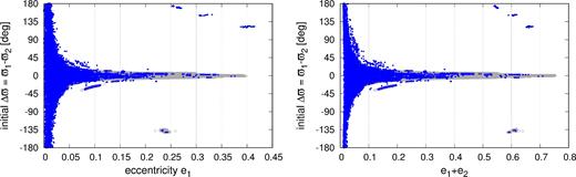
Solutions with L < 0.0145 d (grey dots) derived through optimization of the maximum likelihood function with the GEA. Blue dots are for configurations that result in MEGNO 〈Y〉 ∼ 2 integrated for 64 kyr, indicating regular solutions. Stable, high-eccentricity solutions are visible in small, isolated ‘clumps’, outside a region of Δϖ = 0.
Fig. 1 also illustrates the results of the stability analysis for the models gathered. Due to relatively large masses of ∼6 Earth masses, and close orbits, significant mutual perturbations could be possible. Therefore, for all solutions with L < Lmin we computed their MEGNO signatures for 64 kyr (∼1.8 × 10⁶ outermost orbits). Such an interval well covers the characteristic short-term dynamical time-scale associated with the 9:7 MMR. In the case of the Kepler-29, dynamically stable models may be found in similarly wide range of the parameter plane. Curiously, stable solutions that fit the TTV data exist for e1, 2 as large as 0.3–0.4. Besides the pin-like structure, we also found isolated islands of high-eccentricity solutions beyond the Δϖ = 0 axis. These models could be rather associated with Δϖ librating around π.
Therefore, even if the stability constraints are considered, we actually cannot choose a ‘proper’ or ‘best-fitting’ configuration of the system. More tight constraints are required. At the first step, such constraints may be imposed by a statistical eccentricity distribution expected for compact Kepler systems.
We preformed MCMC experiments to account for the physical limits of (x, y) elements. The results are illustrated in Fig. 2. It shows one- and two-dimensional projections of the posterior probability distribution for Gaussian prior set to (x, y) with zero mean and the variance equal to 0.1. Computations were performed in multi-CPU environment, making it possible to evaluate as much as 1024 000 iterations to avoid the autocorrelation effect. Each run composed of 256 emcee ‘walkers’ initiated in a small ball around low-L solutions found in the GEA search. The posterior is unimodal and centred close to (x, y) ≃ 0 with masses ∼6 M⊕ and ∼5 M⊕ for the inner and outer planet, respectively. The posterior distribution does not change its character, i.e. relatively well-determined peaks when the (x, y)-prior has the variance set to 0.05, 0.1, 0.25 and 0.33, yet the masses are strongly correlated. If the (x, y)-priors are uniform, masses and (x, y)-elements are not constrained.
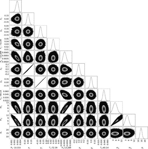
One- and two-dimensional projections of the posterior probability distribution for all free parameters of the TTV model. The MCMC chain length is equivalent to 1024 000 iterations initiated with 256 different instances in a small ball centred at the best-fitting model found with the GEA. The (x1, 2, y1, 2) prior is Gaussian with the zero mean and the variance equal to 0.10. Parameters Ti and Pi are expressed in days, masses mi are expressed in Earth masses (i = 1, 2), and the uncertainty correction term σf is given in minutes. Indices 1 and 2 are for the inner and outer planet, respectively. Contours are for the 16th, 50th and 84th percentile of samples in the posterior distribution. We removed about 10 per cent initial, burn-out samples.
For all (x, y) Gaussian priors, we found strong linear correlations between pairs of (x1, x2) and (y1, y2). These linear correlations could mean a tight alignment of apsidal lines which is a common dynamical feature of the low-order MMRs. This is likely a general effect discussed by Jontof-Hutter et al. (2016) for the first-order MMRs. It may be explained by the evolution of eccentricity vectors [eicos ϖi, eisin ϖi], which are not constrained individually, but their components are tightly correlated.
The results are illustrated in Fig. 3 for three planes of orbital parameters selected from samples with L < 0.0149 d (grey dots). The grey area is filled, as guaranteed by the MCMC sampling, hence we may be confident that the search covers all the relevant parameter space. Solutions with θmin < 1.53 (i.e. with full amplitude ∼1.53 of cos or sin ) are marked with blue filled circles. This experiment shows that solutions with antialigned apsides are preferred for small eccentricities ≃ 0.01, while models with librating critical angles and aligned apsides are found mostly for moderate and large eccentricities.
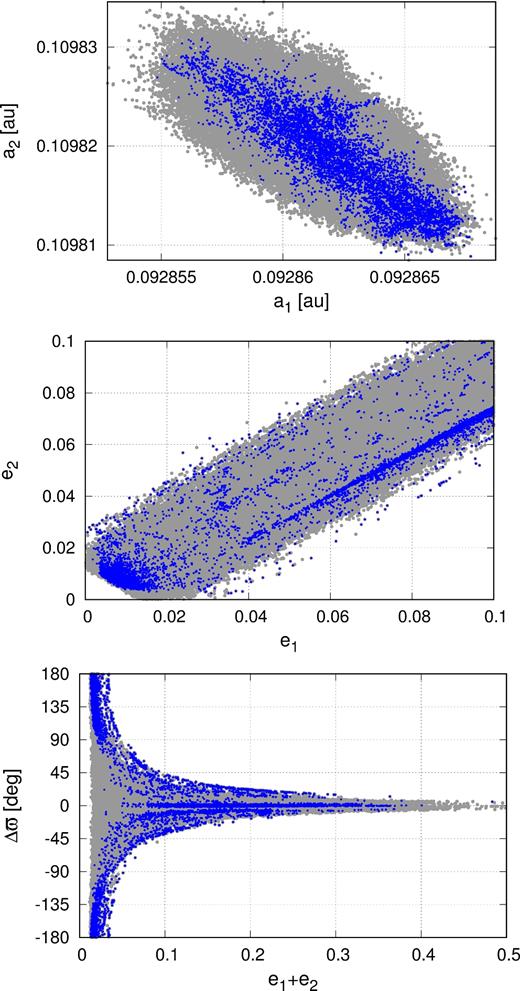
MCMC solutions with L < 0.0149 d (grey filled dots) and with at least one critical argument ϕj, j = 1, 2, 3 librating (blue filled dots). The Gaussian prior for (xi, yi, i = 1, 2) with the zero mean value and the variance equal to 0.1 has been set.
Curiously, the distribution of models in the (e1, e2)-plane forms a strip having a sharp ‘cut-off’ at small eccentricities region (e1 + e2 ∼ 0.01). This effect could be explained by measurable, mutual interactions of the planets. Since the total angular momentum must be conserved, it implies eccentricities variations in antiphase.
2.2 The resonant character of the system
We computed 2-dim dynamical maps in the neighbourhood of two representative best-fitting solutions to visualize the dynamical structure of the 9:7 MMR. First of these solutions is the result of the MCMC sampling for the variance of x1, 2, y1, 2 set to 0.1. Its parameters are given in Table 1 and the synthetic TTV signals are presented in Fig. 4. The top row of Fig. 5 shows dynamical maps in the (a1, e1)-plane for this model. All other orbital elements are kept at their best-fitting values. For each initial condition at the grid, the N-body equations of motion were integrated up to 36 kyr. This corresponds to ∼106 × P2, sufficient to detect short-term chaotic motions for the MMRs instability time-scale (e.g. Goździewski & Migaszewski 2014). As the dynamical maps show, the observational uncertainties of a1 and a2 ≃ 10−5 au are much smaller than the width of the 9:7 MMR, see Fig. 5. The best-fitting solution is found, somehow ironically, just in a narrow unstable structure which may be identified with the separatrix. The 9:7 MMR structure may be even better visible in the right-hand panel of Fig. 5 which is for the frequency map of the system and shows deviations of the ratio of mean motions f2/f1 ≡ n2/n1 (fundamental frequencies) from the exact 9/7 value. The 9:7 MMR spans the middle part of the map, depicted as wide grey/yellow strip of regular motions limited by vertical separatrices. In the middle of this strip, a boomerang-like structure appears with n2/n1 deviations from the 9/7 ratio as small as 10−6 and sharp borders coinciding with curved, narrow separatrices identified in the MEGNO map.
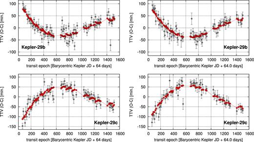
Synthetic TTVs of best-fitting low-eccentricity models for Kepler-29 (Table 1) overplotted on the TTV measurements (red lines are shown merely to guide the reader's eye). The left-hand column presents the fitting results for the data set from Rowe et al. (2015), while the right-hand column is for an example best-fitting model to the data set from Holczer et al. (2016), shown for a reference.
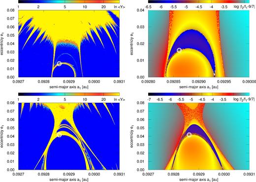
Dynamical maps for the best-fitting TTV models from the MCMC in a region of small eccentricities obtained with Gaussian priors imposed on (xi, yi) parameters with variances of 0.10 ( top row, osculating elements of this model at t0 = KBJD + 64 d are displayed in Table 1) and 0.25 (bottom row), respectively. Left-hand column: dynamical maps in terms of the MEGNO indicator, 〈Y〉 ∼ 2 indicates a regular (long-term stable) solution marked with blue colour, 〈Y〉 much larger than 2, up to ≳ 32 indicates a chaotic solution (orange/red). Integrations done for 36 kyr (roughly 1.2 × 10⁶P2). Right-hand column: deviation of the ratio of fundamental frequencies (mean motions) with respect to the nominal value for the 9:7 MMR, computed for interval spanning 1020 time steps of 0.5 d (≃ 4 × 10⁴P2).
Orbital parameters of a representative TTV model of the Kepler-29 system. The osculating epoch is t0=KBJD+64.0 d. The configuration is coplanar with inclinations I = 90° and nodal longitudes Ω = 0°. Mass of the star is 1.0 M⊙ (Rowe et al. 2015). Elements (x1, x2) and (y1, y2) are strongly correlated pairwise (see Fig. 2).
| Planet | Kepler-29 b | Kepler-29 c |
|---|---|---|
| mp (M⊕) | 5.7|$_{-1.9}^{+1.6}$| | 4.9|$_{-1.6}^{+1.4}$| |
| P (d) | 10.33 585|$_{-0.000\,32}^{+0.000\,39}$| | 13.292 92|$_{-0.000\,69}^{+0.000\,58}$| |
| x ≡ ecos ϖ | 0.0046 ± 0.062 | −0.009 ± 0.05 |
| y ≡ esin ϖ | 0.0154 ± 0.062 | 0.008 ± 0.05 |
| T (d) | 72.4200 ± 0.0041 | 65.1830 ± 0.0048 |
| a (au) | 0.092 8613 | 0.109 8205 |
| e | 0.0160 | 0.01169 |
| ω (deg) | 73.44 | 139.94 |
| |${\cal M}\,$|(deg) | −96.18 | 96.99 |
| σf (d) | 0.009 ± 0.001 | |
| L (d) | 0.0145 | |
We found that the critical angles ϕ1, 2, 3 are not fully adequate signatures of the 9:7 MMR since they may librate with large full amplitudes reaching 2π, even in the boomerang-like region characterized with almost exact 9/7 ratio of the orbital periods.
Yet a highly ordered evolution of (Δϖ, ϕ1) during first 36 kyr (∼106 outermost periods) is illustrated in the top row of Fig. 6 for three initial conditions selected at maps in Fig. 5, with the same elements as the best-fitting model, besides changed e1. The left-hand panel is for e1 = 0.006 (below the lower separatrix of the boomerang-like structure), e1 = 0.019 (close to the nominal solution, between the separatrices) and e1 = 0.026 (above the upper separatrix). In all these cases, a clear resonant behaviour of the system is apparent which we understand here as a strong correlation of the critical angles rather than low-amplitude librations of these critical arguments. The primary indication of the presence of the resonance are the dynamical maps, Fig. 5 and the particular, vertical structure, which is common for MMRs in the (a, e)-plane.
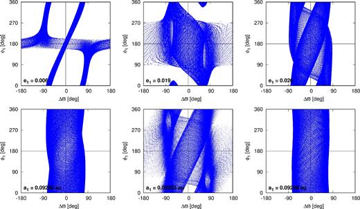
Evolution of critical angles (Δϖ, ϕ1) computed for six initial conditions from a dynamical map in Fig. 5. Integrations interval is 36 kyr. See the text for details.
There is also a clear difference between evolution of the critical angles inside and outside the 9:7 MMR structure. To show this, we integrated two configurations with a1 = 0.092 80 au and a2 = 0.092 98 au (the left- and the right-hand panels of the bottom row of Fig. 6, respectively) that are located outside the resonance. In contrast to highly correlated behaviour of the angles inside the vertical structure, illustrated in the top row of Fig. 6, in both these cases the evolution of the angles is not ordered in the sense explained above. Angle ϕ1 can be equal to 0 or π when Δϖ equals 0. The middle panel in the bottom row illustrates the resonant behaviour, however the initial a1 = 0.092 93 au, so the system is very close to the separatrix between resonant and non-resonant regions. Although the system evolves almost in a whole (Δϖ, ϕ1)-plane, similarly to the top row of Fig. 6, the angles are synchronized and when Δϖ = 0 or π, ϕ1 cannot be 0.
We also found clear semimajor axes oscillations, expected for systems in MMR, whose amplitude is a few times larger in the MMR region, when compared to solutions beyond the MMR structure (not shown here). Moreover, the curved thin chaotic borders encompassing the boomerang-like structure inside the MMR could be identified with separatrices of secondary resonances of the frequency of oscillation of the semimajor axes (the resonant frequency) with the frequency of librations of the secular angle Δϖ (Morbidelli & Moons 1993; Michtchenko & Ferraz-Mello 2001).
The bottom row in Fig. 5 is for the dynamical maps computed for MCMC derived models with the eccentricity priors set to 0.25. This prior leads to systematically larger osculating eccentricities, however the respective posterior distributions look similarly as in Fig. 2. Curiously, the best-fitting solution remains ‘glued’ to the unstable separatrix of the boomerang-like structure.
A problem of constraining the dynamical model of Kepler-29 is finally illustrated in Fig. 7 which shows a MEGNO map for osculating elements from a small island of stable solutions around (e1 ≃ 0.23, Δϖ ≃ −135°), see Fig. 1. Each point in this 〈Y〉 map has been integrated for 64 kyr, which guarantees the Lagrange stability for 10–100 times longer interval, hence for ∼10 Myr. The tested initial condition is found in an island in a kind of archipelago with eccentricities as large as 0.7. Fig. 1 displays a few isolated models of this type with large eccentricities.
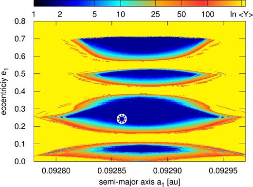
The MEGNO dynamical map for a TTV model in a region of large eccentricities (see Fig. 1) out of Δϖ = 0, computed for 64 kyr (∼2.5 × 10⁶P2). The MEGNO indicator, 〈Y〉 ∼ 2 indicates a regular (long-term stable) solution marked with blue colour, 〈Y〉 much larger than 2, up to ≳ 256 indicates a chaotic solution (light blue/red/yellow).
3 PERIODIC ORBITS
In the previous sections, we could not determine any unique model of the Kepler-29 system with both the observational and dynamical constraints. Therefore, we aim to impose additional constraints through the most likely convergent planetary migration of the system in the past. As it has been shown (Beaugé, Ferraz-Mello & Michtchenko 2003; Beaugé, Michtchenko & Ferraz-Mello 2006; Hadjidemetriou 2006; Migaszewski 2015), systems of two planets that undergo convergent migration evolve along families of periodic orbits. Although the cited papers are devoted to first-order MMRs, one could expect that also for a second-order MMR, like 9:7, periodic orbits play an important role. Therefore, we seek for families of periodic orbits of 9:7 MMR and show where the configurations that fit the TTV data locate with respect to them.
3.1 The representative plane of initial conditions
In order to address those issues, we apply the so called representative (symmetric) plane of initial conditions Σ (e.g. Beaugé & Michtchenko 2003) which makes it possible to illustrate global, qualitative features of the multidimensional and multiparameter planetary systems.
Before introducing the Σ-plane, we recall some essential facts about resonant configurations of two planets in coplanar orbits. Their dynamics may be reduced through the averaging over the fast angles to a two-degree-of-freedom Hamiltonian. This Hamiltonian possesses two first integrals, i.e. the total angular momentum C ≡ G1 + G2 and the so called spacing parameter K ≡ (p + q) L1 + p L2, where |$L_i \equiv \beta _i \, \sqrt{\mu _i \, a_i}$|, |$G_i \equiv L_i \, \sqrt{1 - e_i^2}$|, βi ≡ (1/m0 + 1/mi)−1 and μi ≡ k2(m0 + mi), i = 1, 2 (Michtchenko & Ferraz-Mello 2001; Beaugé & Michtchenko 2003).
The averaged Hamiltonian can be expressed through |$\overline{H} = \overline{H}(I_1, I_2, \sigma _1, \sigma _2; C, K),$| where the canonical variables are Ii = Li − Gi and σi = (1 + s) λ2 − s λ1 − ϖi with s ≡ p/q. It can be shown that |$\mathrm{\partial} \overline{H}/\mathrm{\partial} \sigma _i = 0$| for critical values of (σ1, σ2) = {(0, 0), (0, π), ( ± π/2, ±π/2), ( ± π/2, ∓π/2)}. Therefore, the equilibria of the averaged system, that are periodic configurations of the full three-body problem, do exist for these four pairs of angles. (Note that changing signs for both the angles simultaneously does not lead to any change in the Hamiltonian.) Such configurations are called apsidal corotation resonances (ACR). Here, we consider symmetric ACR only.
The representative (or characteristic) plane of initial conditions Σ is a plane of eccentricities. A point in this plane (e1, e2) determines semimajor axes a1, a2 through the first integrals C and K. The initial condition of a given system contains also angles σ1 and σ2 chosen from the critical set of (σ1, σ2) = {(0, 0), (0, π), ( ± π/2, ±π/2), ( ± π/2, ∓π/2)}. Each orbital configuration with angles (σ1, σ2) that circulate or librate around pairs of critical values given above must intersect this plane (Michtchenko & Ferraz-Mello 2001). Therefore, in order to study the dynamics of such systems globally, it is sufficient to consider the four sets of initial resonant angles (σ1, σ2) in the Σ-plane. However, the Σ-plane defined in this way is representative only for symmetric configurations, for which Δϖ = σ2 − σ1 equals 0 or π. There could, in principle, also exist asymmetric configurations with different libration centres (Beaugé et al. 2003). Since the majority of the best-fitting configurations of the Kepler-29 system are symmetric (apart from, possibly, a few islands with large eccentricities, Fig. 1), we limit our analysis to the symmetric configurations only.
Furthermore, instead of σ1, σ2 we choose their combinations, the secular angle Δϖ and one of the critical arguments of the 9:7 MMR, ϕ1 = −2 σ1, which are more convenient for an interpretation of their evolution. The representative angles at the Σ-plane are then (0, 0), (0, π), (π, 0) and (π, π), and the Σ-plane coordinates can be defined as (e1 cos Δϖ, e2cos ϕ1), where both cosines are equal to +1 or to −1.
Although the Σ-plane has been defined for the averaged Hamiltonian with two degrees of freedom, we can use the same concept also for the full three-body, non-averaged system. It is convenient to show orbital models that fit the observations with respect to the periodic orbits represented as equilibria of the averaged system.
3.2 TTV-constrained models in the Σ-plane
We narrowed the set of dynamically stable initial conditions, as illustrated in Fig. 3, by L < 0.0145 d. To map this set on the Σ-plane, we integrated the N-body equations of motion forward for 105 yr. Each time when ε ≡ ‖sin Δϖ‖ + ‖sin ϕ1‖ ≲ 0.02 (expressed in radians; for numerical reasons of limited integration time, we chose a small limit of ε = 0.02 for the intersection of the Σ-plane), osculating elements were transformed to coordinates at the Σ-plane and presented in the left-hand panel of Fig. 8. Usually, each initial configuration evolving in time results in more than one point at this plane. For the reduced system with two degrees of freedom one obtains: (i) one point at the Σ-plane if the system is in a stable equilibrium; (ii) two points if it is a stable periodic configuration of the reduced system (fixed point at the Poincaré cross-section); (iii) four points if the reduced system evolves along quasi-periodic orbit; (iv) a continuum of points for chaotic evolution. The full (non-averaged) system intersects the Σ plane in four groups of points if its reduced counterpart intersects the plane in four points.
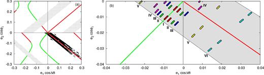
Panel (a): the best-fitting solutions from the TTV analysis (Figs 1 and 3) projected at the representative plane (black points). We consider a given configuration as crossing the plane if Δϖ and ϕ1 differ from the nominal values of 0 or π by less than one degree. Green and red curves denote families of stable and unstable periodic configurations of the N-body system, respectively. Grey symbols denote configurations for which the closest encounter of the planets in Keplerian orbits is smaller than 3 Hill radii (≈0.005 au). Panel (b): chosen configurations (whose parameters are listed in Table 2) projected at the representative plane in the same manner as for the whole statistics of systems presented in panel (a). Each configuration is plotted in different colour and labelled. Only bottom half of the Σ-plane is shown. The grey filled area shows qualitatively the black strip of points shown in panel (a).
As Fig. 8 shows, stable models that fit the TTV data form a strip at the Σ-plane along a line originating from (0, 0) and directed towards higher eccentricities in the quarter of the plane with Δϖ = 0 and ϕ1 = π. There are points in the (Δϖ, ϕ1) = (π, π)-quarter as well, but no configurations intersect the upper half of the Σ-plane (ϕ1 = 0).
The second critical component of Fig. 8 is a representation of families of the periodic orbits. Green and red solid curves show families of stable and unstable equilibria of the reduced system (periodic configurations of the full system), respectively. The periodic system returns to its initial state after a certain period P. For the periodic orbits in the 9:7 MMR, it covers nine revolutions of the inner planet, and seven revolutions of the outer planet. Then the planets starting for instance from their pericentres will be back in the pericentres after the period P. Also orbital elements |${\pmb {p}} = (a_1, a_2, e_1, e_2, \mathcal {M}_1, \mathcal {M}_2, \Delta \varpi )$| will retain their initial values. Angles ϖ1 and ϖ2 will change, since the system precesses as a whole. For a given point (e1, e2), we integrate the equations of motion and evaluate |$\delta = \Vert {\pmb {p}}(t=T) - {\pmb {p}}(t=0) \Vert$|. We search for such (e1, e2) (for a given C, K) that provides δ ≃ 0. In order to check the stability of a given periodic configuration, we integrate the system for ∼105 revolutions. A stable periodic configuration is preserved, while for unstable one, sooner or later the system evolves into different regions of the phase space.
Apparently, the best-fitting solutions appear along a family of unstable equilibria. We found this result somehow unexpected from the point of view of the formation of the system through the migration. Unstable periodic orbits in the proximity of the observationally constrained configurations may be also a factor provoking dynamical instability of the system. Although aligned configurations are, in general, not impossible to form within the migration formation scenario (e.g. Beaugé et al. 2003; Ferraz-Mello et al. 2003), the aligned configurations studied in the cited papers are related to the branch of stable equilibria. As shown in the previous section, geometrical parameters of the system like eccentricities and pericentre longitudes are not well constrained due to low signal-to-noise ratio, narrow observational window and features of the TTV method. This permits us to look for solutions fulfilling also the migration constraints.
As Migaszewski (2015) has demonstrated, two-planet systems that undergo convergent migration end up in exact periodic configurations. Nevertheless, that conclusion referred to the first-order resonances and might not be fully applicable to the second-order MMRs. We will discuss this further in this paper. After inspecting the O-C diagrams of Kepler-29 system (see Fig. 4), one can conclude that it cannot be related to exactly periodic configurations. In such a case, there would be no secular TTV signal of a period longer than the resonant period of ≃ 91 d. However, such a signal of a few-year period is clearly visible in the data. Therefore, the real Kepler-29 cannot be a strictly periodic configuration. Nevertheless, we show further that the migration is still very likely a way the system has been formed.
3.3 Particular solutions in the Σ-plane
The right-hand panel of Fig. 8 illustrates models selected from the set of solutions that well reproduce the observations. Those six models (Table 2) were chosen as qualitative representatives for all the statistics of the best-fitting models. Model I (red points) intersects the Σ-plane very close to the branch of stable equilibria and all four groups of points where the system intersects the Σ-plane lie in the (Δϖ, ϕ1) = (π, π) quarter. Model III (blue points) lies further from the stable branch than Model I, and its phase trajectory intersects both quarters with ϕ1 = π. Model II (green points) is an intermediate configuration between Models I and III. Its phase trajectory almost ‘touches’ the quarter with Δϖ = 0. Model VI (cyan points) lies in vicinity of the unstable branch of equilibria in the (0, π)-quarter and intersects only this quarter. Models IV (magenta points) and V (yellow points) are intermediate states between Models III and VI. The sequence of models from I to VI shows a transition between configurations very close to the branch of stable equilibria and configurations close to the branch of unstable equilibria.
Parameters of six selected models that fit the TTV measurements and exhibit different qualitative orbital behaviour (see the text for details). The osculating Keplerian elements are given at the epoch of t0 = BJKD + 64.0 d. The system is coplanar with I = 90° and Ω = 0°. Mass of the parent star is 1 M⊙.
| Model/pl | m (M⊕) | a (au) | e | ϖ (deg) | |$\mathcal {M}$| (deg) |
|---|---|---|---|---|---|
| I/b | 7.5173 | 0.092 8595 | 0.005 42 | 18.30 | −40.97 |
| I/c | 6.5125 | 0.109 8237 | 0.008 09 | −148.75 | −334.13 |
| II/b | 6.2177 | 0.092 8608 | 0.006 29 | 0.15 | −22.62 |
| II/c | 5.4607 | 0.109 8212 | 0.008 91 | −138.86 | −343.92 |
| III/b | 7.5940 | 0.092 8594 | 0.007 58 | 58.44 | −81.28 |
| III/c | 6.6879 | 0.109 8237 | 0.007 76 | 179.74 | 57.30 |
| IV/b | 7.2520 | 0.092 8609 | 0.010 68 | 9.75 | −31.75 |
| IV/c | 6.0265 | 0.109 8228 | 0.004 72 | −117.62 | −4.75 |
| V/b | 5.1439 | 0.092 8622 | 0.014 89 | 84.22 | −107.33 |
| V/c | 4.4826 | 0.109 8190 | 0.013 88 | 149.42 | 87.16 |
| VI/b | 5.9161 | 0.092 8578 | 0.017 90 | 155.65 | −181.05 |
| VI/c | 6.1775 | 0.109 8202 | 0.027 34 | 177.86 | 56.85 |
Fig. 9 shows the orbital evolution of the selected models at the (Δϖ, ϕ1)-plane. Both angles of Fit I librate around π, although the amplitude of ϕ1 libration is large. For the second model in the test sample (Fit II), the ϕ1 libration amplitude reaches 2π, while Δϖ librates with a moderate amplitude. Since the amplitude of ϕ1(t) is actually greater than 2π, we could classify the behaviour of this angle as circulation. Despite the formal rotation of ϕ1, the phase-space trajectory of Fit II intersects only one quarter of Σ −plane with (Δϖ, ϕ1) = (π, π). The next Fit III in the sample exhibits both critical angles rotating and two quarters of Σ −plane are intersected by the phase trajectory. Two other quarters are being avoided. Similarly, the phase trajectory of Fit IV intersects the same two quarters of Σ −plane. Yet the behaviour of the angles is different. For Fit IV, ϕ1 seems to librate but with an amplitude larger than 2π. The next system, Fit V, shows both angles circulating, however in this case Δϖ remains mainly around 0 during the evolution, only occasionally reaching π. The last model, Fit VI, has Δϖ librating around 0 and ϕ1 circulating.
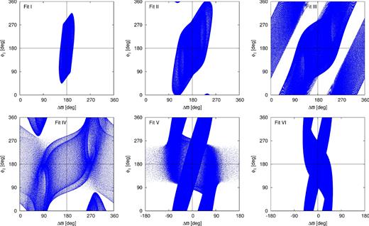
Evolution of example configurations that fit the data (see Table 2 for the masses and orbital parameters) presented at the (Δϖ, ϕ1)-diagram. The integration time is 105 yr.
Similarly to Fig. 8, Fig. 9 also reveals the transition between two different types of configurations (from Fit I to Fit VI). The sequence of the configurations can be also analysed in energy plots of the averaged system presented in Fig. 10. Mean orbital parameters of Fit I to Fit VI are displayed in Table 3.
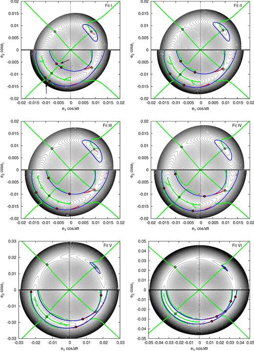
Energy levels (black curves) of the averaged system at the Σ-plane. Masses and the C and K integrals values are for the selected configurations (see Table 3 for the parameters). Each panel is for one of the six models chosen for the analysis. Blue curves are for energies of the nominal systems. Green and red curves denote periodic configurations of the averaged model, while black cross-circle symbols are for the periodic configurations of the N-body (unaveraged) model, i.e. equilibria of the averaged system. Big red symbols show intersections of the representative plane by the trajectories of the nominal systems.
Mean parameters of the selected configurations whose osculating Keplerian elements are given in Table 2.
| Solution/planet | m (M⊕) | a (au) | e | σ (deg) |
|---|---|---|---|---|
| I/b | 7.5173 | 0.092 8783 | 0.006 02 | 53.16 |
| I/c | 6.5125 | 0.109 8163 | 0.008 71 | 220.76 |
| II/b | 6.2177 | 0.092 8756 | 0.006 91 | 68.06 |
| II/c | 5.4607 | 0.109 8110 | 0.009 27 | 209.73 |
| III/b | 7.5940 | 0.092 8799 | 0.007 79 | 12.87 |
| III/c | 6.6879 | 0.109 8067 | 0.008 62 | −111.90 |
| IV/b | 7.2520 | 0.092 8714 | 0.011 26 | 58.13 |
| IV/c | 6.0265 | 0.109 8052 | 0.004 91 | 193.85 |
| V/b | 5.1439 | 0.092 8691 | 0.014 70 | −16.53 |
| V/c | 4.4826 | 0.109 8080 | 0.014 50 | −84.06 |
| VI/b | 5.9161 | 0.092 8795 | 0.017 24 | 89.52 |
| VI/c | 6.1775 | 0.109 8070 | 0.027 97 | 68.22 |
A given energy plot is constructed for values of the two integrals C and K computed for each studied system. The energy of each system is determined by the averaged Hamiltonian (see Appendix A). Energy levels are plotted in the Σ-plane. The energy level for the nominal system is plotted with blue solid curve, while black solid curves are for other values of the energy, from the maximum of the energy that corresponds to the stable equilibrium (black cross-circle symbol in the (π, π)-quarter of Σ-plane), down to smaller values. The energy levels are limited from the bottom by |$\overline{H}(e_1=0, e_2=0)$|. The levels could also be plotted for smaller values, although these levels would become subsequently denser and they would be placed further from the centre of the plane. Other three cross-circle symbols in the remaining quarters represent positions of the unstable equilibria.
Let us recall that Fig. 8 shows positions of equilibria of the averaged system (periodic orbits of the full, non-averaged N-body model of motion) computed not for one particular value of C, like in Fig. 10, but for a series of values. This leads to whole branches/families of equilibria shown with green and red curves for stable and unstable equilibria, respectively. On contrary, green and red curves in Fig. 10 represent periodic orbits of the averaged system, green are for stable, while red for unstable configurations. Big red/black symbols point where the nominal systems intersect the Σ-planes. The points of intersections can be compared with the ones in the right-hand panel of Fig. 8. Small differences are present between the results of the N-body and the averaged model, which may be easily explained. The averaged model is of the first-order with respect to the perturbation, which do not have to be necessarily small for such a compact two-planet system. Nevertheless, a sequence of models from Fit I (close to the stable equilibrium) to Fit VI (close to the unstable equilibrium) is apparent here as well.
A common feature of all the models is a close proximity of their nominal energy curves to the bifurcation of the branches of periodic orbits of the averaged system in the (π, π)-quarter (see the arrows in the top-left panel of Fig. 10). Moreover, the energy values are just below the critical energy of the saddle point in the (0, π)-quarter. Naturally, those two characteristics of the energy for the nominal systems are not independent one from another, since the structure of periodic orbits is determined by positions of the equilibria. This feature may be a ‘fingerprint’ of the migration scenario, which we discuss in the next section.
4 PLANETARY MIGRATION
After a series of simulations, we found the following properties of systems stemming from the migration. For small κ ≲ 10, moderate and high eccentricities (≳ 0.03) were possible to obtain, however Δϖ librates around π, which is opposite to the results of fitting the data. Additionally, such systems have always ϕ1 librating around π. Both the angles librate around π. For moderate κ ∼ 100, small eccentricities ≲ 0.01 are obtained and Δϖ spans the whole range, revealing both librations around π or circulations, which agrees with the statistics of models that fit the data.
Next, we tried to find configurations resulting from the convergent migration, which could form the sequence of six models analysed in the previous section. They should transform from one class of configurations (close to the stable equilibrium) to another class (close to the unstable equilibrium).
After a series of experiments, we found that three out of six models could be qualitatively reconstructed by a single migration simulation. The results of such a simulation are illustrated in Fig. 11. Its parameters as well as the initial orbital elements are given in the caption to this figure. Subsequent panels, from the top to the bottom, correspond to the period ratio, eccentricities, Δϖ and ϕ1 evolution in time. Shortly after the system reaches the 9:7 MMR, the eccentricities are excited, i.e. e1 oscillates in a range of [0.004, 0.008] and e2 ∈ [0.006, 0.01]. Both critical angles librate around π, Δϖ with very small amplitude <1°, while ϕ1 with much larger amplitude of ∼70°. Both the amplitudes increase in the first part of the simulation t < 125 kyr. If the migration has stopped for some reason at this stage of the evolution, Δϖ would librate with too small amplitude, when compared to the examples listed in Table 2 and also to the systems from the whole statistics of the TTV fits.
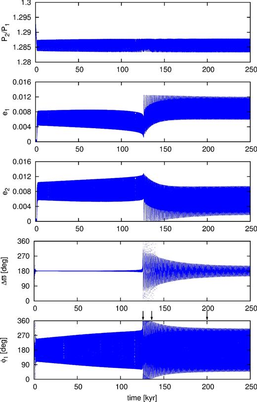
An example of the migration simulation which leads to systems similar to Kepler-29. Initial semimajor axes are a1 = 0.2 au and a2 = 0.237 23 au, eccentricities e1 = e2 = 0.0001, both arguments of pericentre and mean anomalies are set to 0. Planets masses are m1 = 5.1 M⊕ and m2 = 4.4 M⊕. Parameters of the migration τ0 = 12 kyr, T = 40 kyr, α = 1.3, κ = 130.
At t ∼ 125 kyr, the system switches into a different regime of motion. Both Δϖ and ϕ1 start to circulate, the ranges of the eccentricities oscillations also change. After ∼10 kyr since the transition (at t ∼ 135 kyr), the angles start to librate again with decreasing amplitudes. One should keep in mind, though, that it is not a generic situation. If T had a higher value (which would mimic slower disc dispersion), the system would leave the resonance eventually. If, on the other hand, T was smaller, the migration could stop before the transition between the two discussed regimes of motion.
More details about the evolution of a system trapped in 9:7 MMR could be found in our upcoming paper. Here, we only present an example showing that systems listed in Table 2 can be formed through the migration. A critical issue is the transition described above. It occurs if the energy of the migrating system reaches the bifurcation of the branches of periodic orbits (see the arrows in the top-left panel of Fig. 10).
We chose three moments of the simulation, t = 126, 136 and 200 kyr, respectively, and we integrated the N-body equations of motion for the three sets of the osculating Keplerian elements at those epochs. Snapshots of their evolution are presented at the (Δϖ, ϕ1)-diagrams in Fig. 12.
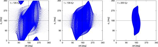
Evolution of example configurations stemming from the migration simulation illustrated in Fig. 11, presented at the (Δϖ, ϕ1)-diagram. The integration time is 105 yr.
The left-hand panel reminds the bottom-left panel of Fig. 9 (Fit IV) as well as the middle panel of Fig. 5 for the observational model close to the best-fitting solution in Table 1. Both the angles formally circulate, however, similarly to Fit IV, ϕ1 librates with the amplitude greater than 2π. The evolution of the angles is not independent one from another, since the phase trajectory avoids certain areas of the (Δϖ, ϕ1)-diagram. The right-hand panel of Fig. 12 reminds the top-left panel of Fig. 9 (Fit I). Both the angles librate and the amplitudes for the simulated system correspond well to the amplitudes for Fit I. The system in the middle panel can be interpreted as an intermediate state between the systems illustrated in the left- and right-hand panels of Fig. 12. The amplitude of ϕ1 libration reaches 2π, which corresponds to the behaviour of Fit II (the top middle panel of Fig. 9). The only difference between the simulated system and Fit II is the behaviour of Δϖ. Yet we also note that the evolution of critical angles for Fits V and VI is very similar to the observational models illustrated in the left- and right-hand panels of Fig. 6.
The examples stemming from the migration simulation ensure us that the Kepler-29 system could be formed by the planetary migration if its orbits are close to circular. On the other hand, the systems with higher eccentricities (and aligned orbits) which are also consistent with the TTV observations are less likely to be formed in this way. Nevertheless, the migration induced formation of the 9:7 MMR as well as other second-order and higher order resonances is a very complex mechanism. It needs to be studied in more detail in order to bring a definitive solution.
5 CONCLUSIONS
We analysed the TTV data from Rowe et al. (2015) of the Kepler-29 system with two low-mass planets of a period ratio very close to 9/7 (Jontof-Hutter et al. 2016). We confirmed that the masses of the planets are within a few Earth mass range, i.e. ∼6 M⊕ and ∼5 M⊕ for the inner and the outer planet, respectively. We demonstrated that, although the eccentricities as well as longitudes of pericentres are not well determined, the system is very likely in an exact 9:7 MMR. We found configurations with both aligned and antialigned apsides, that are long-term stable and fit the data equally well. The eccentricities may be as high as 0.3–0.4 for models with aligned orbits, while for antialigned configurations only low eccentric orbits are allowed by the observational and stability constraints.
We demonstrated that the critical angles of the resonant configurations do not necessarily librate. That also implies that the secular angle Δϖ may both rotate or librate, around 0 or π. The resonant nature of such systems can be verified at the frequency maps (right-hand column of Fig. 5) as well as at the (Δϖ, ϕ1)-diagrams (Fig. 9). The fundamental frequencies related to the mean motions are very close to the nominal value of 9/7 for the systems whose resonant angles rotate. Moreover, the evolution of the angles Δϖ and ϕ1 is correlated.
We showed that the best-fitting solutions with low eccentricities (both with aligned and antialigned apsides) are shifted with respect to the periodic orbits (equilibria of the averaged system) of 9:7 MMRs, and demonstrated that it is a natural outcome of the planetary migration. That holds even for configurations that lie close to the branch unstable periodic orbits for Δϖ = 0 (Fit IV). On the other hand, we showed that configurations with e ≳ 0.03 and Δϖ ∼ 0 are unlikely to be formed on the way of migration. Systems with e ≳ 0.03 and Δϖ ∼ π can form this way, but configurations of this sort do not fit the TTV observations. Therefore, we conclude that if the Kepler-29 system was formed through the smooth migration, its orbits are low eccentric e ≲ 0.03, but the behaviour of Δϖ and the resonant angles can be hardly determined on basis of the available TTV data.
Acknowledgments
We would like to thank the anonymous referee for helpful suggestions that helped us to improve the paper. We thank Ewa Szuszkiewicz, John Papaloizou and Zija Cui for discussions stimulating our interest in the Kepler-29 dynamics. This work has been supported by Polish National Science Centre MAESTRO grant DEC-2012/06/A/ST9/00276. KG thanks the staff of the Poznań Supercomputer and Network Centre (PCSS, Poland) for a generous support and computing resources (grant no. 195).
REFERENCES
APPENDIX A: ANALYTIC 9:7 MMR HAMILTONIAN
The secular and the resonant parts of the averaged Hamiltonian (equation 3) read as follows (Murray & Dermott 1999).
