


Abstract
We study the dynamical evolution of the putative gas clouds G1 and G2 recently discovered in the Galactic Centre. Following earlier studies suggesting that these two clouds are part of a larger gas streamer, we combine their orbits into a single trajectory. Since the gas clouds experience a drag force from background gas, this trajectory is not exactly Keplerian. Assuming the G1 and G2 clouds trace this trajectory, we fit for the drag force they experience and thus extract information about the accretion flow at a distance of thousands of Schwarzschild radii from the black hole. This range of radii is important for theories of black hole accretion, but is currently unconstrained by observations. In this paper, we extend our previous work by accounting for radial forces due to possible inflow or outflow of the background gas. Such radial forces drive precession in the orbital plane, allowing a slightly better fit to the G1 and G2 data. This precession delays the pericentre passage of G2 by 4–5 months relative to estimates derived from a Keplerian orbital fit; if it proves possible to identify the pericentre time observationally, this enables an immediate test of whether G1 and G2 are gas clouds part of a larger gas streamer. If G2 is indeed a gas cloud, its closest approach likely occurred in late summer 2014, after many of the observing campaigns monitoring G2's anticipated pericentre passage ended. We discuss how this affects interpretation of the G2 observations.
1 INTRODUCTION
Sgr A*, the black hole in the centre of our Galaxy, is our closest example of an accreting supermassive black hole. Even in this nearby example, important aspects about how gas makes its way to the black hole remain unknown. For example, the accretion rate at ∼100 Rs1 (inferred from radio observations) is less than ∼1 per cent of the accretion rate at the Bondi radius (∼105 Rs) inferred from X-ray observations (Quataert & Gruzinov 2000b). Thus, only a tiny fraction of the gas bound to the black hole makes its way to the event horizon.
Several models have been proposed to explain this reduction in accretion rate. Examples include ADIOS models, which expel most of the gas in a strong outflow (Blandford & Begelman 1999), CDAF models, which recycle gas outwards in large-scale convection cells while the gas remains gravitationally bound (Quataert & Gruzinov 2000a) and magnetically arrested models (MAD), in which magnetic forces inhibit radial inflow (e.g. Narayan, Igumenshchev & Abramowicz 2003). Tests at radii intermediate between the event horizon and the Bondi radius, ∼103–104 Rs are crucial to distinguish among these various accretion theories, yet there are few probes of this region. Recent infrared observations have identified low-mass gas clouds, G1 and G2, moving through this exact region. Measuring their interaction with the background gas could therefore provide important information about black hole accretion physics (e.g. Narayan, Özel & Sironi 2012).
Such interaction could take the form of a drag force, which would modify the orbits of the clouds and cause deviations from a Keplerian trajectory. These deviations are unfortunately too small to unambiguously identify in the published data for the individual clouds, which span only a few years. Since G1 and G2 are on strikingly similar, though slightly different, orbits about the black hole (Gillessen et al. 2012; Phifer et al. 2013; Pfuhl et al. 2015), we instead work with the assumption that G1 and G2 are part of a larger gas streamer (from, e.g., a partial tidal disruption; Guillochon et al. 2014), and therefore trace different parts of the same trajectory.
We therefore assume that G1 represents the future evolution of G2; this assumption makes specific predictions, testable on an ∼3–5 yr time-scale, or possibly (as we discuss in this paper) with data that are currently available.
First proposed by Pfuhl et al. (2015), this assumption that G1 and G2 follow the same trajectory effectively extends the length of observations by ∼13 yr and significantly expands our ability to constrain its long-term evolution. In McCourt & Madigan (2016) (hereafter MM16), we used this assumption to constrain the rotation axis of the accretion flow surrounding Sgr A*. We found a rotation axis similar to that of the Galaxy; this is consistent with the circumnuclear disc, with the Fermi bubbles, with a possible X-ray jet in the Galactic centre and with available constraints from the Event Horizon Telescope (see MM16 for references and details).
This paper builds on the analysis presented in MM16 by allowing for possible inflow or outflow in the background accretion flow. We show that the data favour inflow along the trajectory, which drives precession of the eccentricity vector and provides a slightly better fit to the data. This effect is equivalent to delaying G2's pericentre passage by ∼5 months from predictions based on a Keplerian fit to the orbit (e.g. Gillessen et al. 2013b; Phifer et al. 2013).
2 METHOD
As discussed in the introduction, we assume that G1 and G2 are part of a coherent gas streamer, with G1 preceding G2 by a time-lag of about ∼13 yr (which we fit for). We therefore assume the two clouds follow a single trajectory. This trajectory would be a Kepler orbit if the clouds moved through a vacuum, but deviates due to drag forces from the ambient gas in the accretion flow. We use the inferred changes in their orbits to probe the accretion flow around the supermassive black hole, Sgr A*. This analysis is discussed in Pfuhl et al. (2015) and again in MM16; we do not describe it in detail here.
We numerically integrate trajectories for a gas cloud starting from an initial condition, varying the parameters in the model for the accretion flow. We estimate the likelihood of each trajectory by comparing it against the astrometry and velocity data published in Gillessen et al. (2013a,b) and in Pfuhl et al. (2015). We maximize this likelihood over all free parameters for the accretion flow, using the emcee MCMC optimizer (Foreman-Mackey et al. 2013). Our methodology is described in detail in MM16 and our code is publicly available online.2
3 RESULTS
We compare our model results with astrometric and velocity data in Fig. 1. Due to uncertainty in the background model, we obtain a family of degenerate solutions which all fit the data, shown as a ‘bundle’ of thin black lines (we show the parameter distributions from our MCMC chain in the appendix). Our predictions would become far more specific if we were to adopt a particular accretion model, e. g. an ADAF (Narayan & Yi 1994). We do obtain a better fit to the data than MM16: the χ2 per degree of freedom (d.o.f.) improves to χ2/d.o.f = {3.1, 0.82} from {4.1, 2.8} when we allow for inflow in our model of the background medium. In both cases, the first number is a standard χ2 calculated using the uncertainties quoted in Gillessen et al. (2013a,b) and Pfuhl et al. (2015), and the second number is calculated including an additional systematic uncertainty derived self-consistently from the data (see equation 7 in MM16).
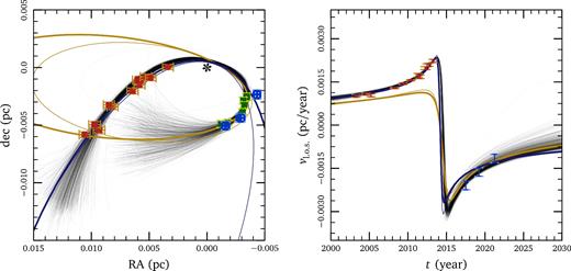
Left: comparison of our model results with astrometric data. Thin black lines show a random sample of models drawn from our MCMC chain. Red points indicate Br-γ observations of G2 from Gillessen et al. (2013b), while the green and blue points show the L-band and Br-γ observations of G1 from Pfuhl et al. (2015). Smaller, dark error bars correspond to those reported in the observational papers. Larger error bars include the systematic error found from our maximum-likelihood analysis (see MM16 for details). Coloured ellipses show Keplerian orbits fit to G1 (yellow) and G2 (blue). Thick lines show the fits we derived in MM16, and thin lines show the fits described in Gillessen et al. (2013b) and in Pfuhl et al. (2015); the differences between them provides a measure of the uncertainty in the fitting. The location of Sgr A* is marked with an asterisk. Right: comparison of our models with line-of-sight velocity. As in the astrometry plot, the smaller error bars are from Gillessen et al. (2013b) and Pfuhl et al. (2015), while the larger ones account for the systematic error determined by our maximum-likelihood analysis. The G1 data points (blue error bars) and Kepler fits (yellow curves) are shifted by 13 yr to compare with our models (cf. Pfuhl et al. 2015).
Fig. 2 compares the eccentricity vector precession in our simulations with the G1 and G2 data. This can be seen by either the argument of pericentre ω (top panel) or more directly by the rotation angle ie (bottom panel), defined in Madigan & McCourt (2016).3 Shaded regions show the 1σ and 2σ spread in our models; yellow curves show results from MM16 which do not include inflow or outflow, blue curves show results from our updated model. Models without inflow have almost no net precession; the implied precession derived from Kepler fits to G1 and G2 data (black error bars, or grey band) is much greater than can be accommodated in these models. Models with inflow can easily reproduce this precession, however (see Appendix A for a discussion connecting precession to inflow). We note that this is a crude comparison to the data since our model provides a better fit to the data than the separate Kepler fits used to infer observational values for ω or for ie; Fig. 2 nonetheless illustrates the key difference between our models and the models from MM16, which did not allow for inflow or outflow in the background: we find that inflow drives prograde precession of the orbit, thus enabling a better fit to the data.
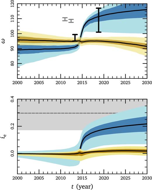
Precession in models with (blue) and without (yellow) inflow. Shaded regions indicate 1σ and 2σ quantiles. Top: argument of pericentre ω for the osculating orbit. Over the 30 yr shown, its evolution is strongly peaked at pericentre. Bottom: integrated effect of precession expressed as the rotation angle ie in radians (see footnote 3, or Madigan & McCourt 2016 for the definition). The grey band shows a crude estimate derived from Kepler fits to G1 and G2 in Pfuhl et al. (2015) and in Gillessen et al. (2013b). Models from MM16 (yellow) do not reproduce this precession.
Physically, prograde precession implies a delay in the pericentre passage of the orbit. Fig. 3 shows this explicitly, and demonstrates that the predicted pericentre time of G2's orbit is model dependent (even among models which fit the available data). Models with different precession rates can move the pericentre time by many months; this is far greater than the statistical uncertainty from fitting the data with any given model. Fitting a purely Keplerian orbit to the G2 data yields the earliest estimate of G2's pericentre passage in 2014 March–April4 (Gillessen et al. 2013b). The distribution shifts by several months if we include a drag force, peaking 2014 mid-June for models with no inflow, and 2014 early August for models with inflow.
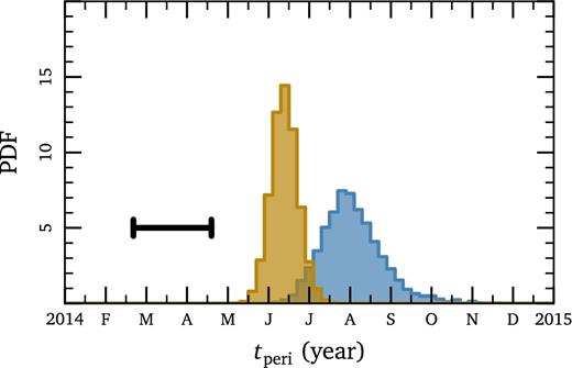
Pericentre times derived for G2. The prograde eccentricity vector precession seen in models with inflow (blue) implies a later pericentre time than models without inflow (yellow), as is expected. The error bar shows the pericentre time derived for a Kepler orbit, which is earlier by many months.
Witzel et al. (2014) report four new epochs of near-infrared imaging of G2 taken from 2014 March through early-August. They constrain the size of G2 in the L΄-band in each epoch, finding that it remains compact through the summer of 2014. Based on the pericentre time expected for a Keplerian orbit, they conclude that G2 has survived its closest approach to Sgr A*. We note however, that given the precession implied by comparing G1 and G2, the data in Witzel et al. (2014) could very well have been entirely taken pre-pericentre. If it proves possible to identify the pericentre passage observationally to within ∼ 2 months, which could definitively determine whether G2 is an ∼ Earth-mass cloud or a stellar-mass source. In principle, this test should be possible using existing data.5
We note that G1's pericentre time is also model dependent. However, the statistical uncertainty due to the limited data dwarfs the systematic differences between models. All models are consistent with G1 passing pericentre at essentially any time in 2001.
We find that our models generically prefer inflow (as opposed to outflow) of the background gas; inflow causes prograde precession near pericentre which better fits the orbits of G1 and G2 (we discuss how inflow and outflow influence orbits in the appendix). If most of the gas in the accretion flow ultimately moves outwards in a wind (as is likely to be the case; Narayan & Yi 1994; Blandford & Begelman 1999; Quataert 2004; Wang et al. 2013), this outflow cannot cover the entire range of angles. Since G2's orbit is misaligned with the rotation axis of the background gas, we find tentative evidence for a geometrically thick disc with an opening angle of at least 30|$^\circ$|–50|$^\circ$|, broadly consistent with a radiatively inefficient accretion flow. This is only a tentative result at the moment, however: the magnitude of the inflow is degenerate with other parameters and the effect may be model dependent. It is also possible that a different model, with a non-Keplerian rotation profile (e.g. Pen, Matzner & Wong 2003), could match the observational data without inflow. This result nonetheless demonstrates the potential power of using the G1 and G2 clouds to probe the Galactic centre accretion flow.
4 DISCUSSION
The G1 and G2 clouds are on strikingly similar, but slightly different, orbits around the supermassive black hole in our Galactic centre. We interpret these clouds as part of a larger gas streamer; the slight differences in their orbital parameters therefore represent evolution of the trajectory due to interaction with the background gas (Pfuhl et al. 2015; McCourt & Madigan 2016). If this picture proves correct, the ‘G-clouds’ can be used to probe the accretion flow feeding Sgr A* at distances of thousands of Schwarzschild radii, a critical range for accretion physics which is currently unconstrained by observations.
In this paper, we build upon the work in MM16, updating our accretion flow model to include a radial component due to inflow or outflow. Near pericentre, this radial component drives rapid precession of the orbit, effectively delaying the pericentre time by up to ∼5 months relative to predictions based on a Keplerian orbit (see Fig. 3). As in MM16, we find that we can only fit the data for G1 and G2 if the clouds are elongated and if the background accretion flow rotates. Uncertainties in the mass and shape of the cloud prevent a determination of the exact properties of the accretion flow; instead, we obtain a degenerate family of models which all fit the data. We furthermore neglect evolution in the size and shape of G2, which would magnify both the drag force on the cloud, and its expected anisotropy. This would in turn flatten the radial profiles we infer for the background density and velocity, and is essential for quantitative constraints on the Sgr A* accretion flow. While these changes may be of the same order as the inflow/outflow we consider in this paper, we do not expect them to change the sign of our results. This paper merely highlights that adding an extra, persistent radial force leads to qualitatively distinct precession of the orbit; this effect might be expected in an accretion flow, and appears to be consistent with the observations. We derive a rotation axis close to both the Galaxy's rotation axis and to the circumnuclear disc. This axis is consistent with that found in MM16.
We find that models with inflow better match the data; inflow causes prograde precession of the eccentricity vector near pericentre which is implied by comparing the orbits of G1 and G2, |$(\boldsymbol {e}_{\text{G}1} - \boldsymbol {e}_{\text{G}2})\cdot \boldsymbol {v}_{\text{G}2} > 0$| (see Appendix A for definitions and details). The magnitude of the inflow is degenerate with several other parameters however. We find tentative evidence for a geometrically thick accretion disc with an opening angle of at least 30|$^\circ$|–50|$^\circ$|, broadly consistent with radiatively inefficient accretion flow models. There are a number of observations that can test our model and our assumptions.
The pericentre time for G2 should be delayed by ∼5 months behind the prediction based on a Kepler orbit. Though the pericentre passage may be difficult to discern precisely from the data, such a test has the advantage that it could be performed immediately, and with existing data sets.
The post-pericentre evolution of G2's orbit should look like G1's in the coming ∼3–10 yr (though differences in mass, shape and size of the two gas clouds may translate to a slightly different evolution).6
G1's orbit should continue to circularize and reorient to align with the accretion flow axis. The time-scale for this is likely to be decades, however, unless G1 expands significantly.
‘Older’ clouds (those preceding G1, which have interacted with the accretion flow for a longer time), if they exist, should be less eccentric, have smaller semimajor axes and have angular momentum vectors increasingly aligned with the accretion flow.
A number of observing campaigns monitored the Galactic centre during February–May of 2014, when the cloud was predicted to pass pericentre. If G2 is in fact a gas cloud, however, its pericentre passage was likely several months afterwards, in late summer of 2014. Many observing campaigns unfortunately ended before this date.
Ponti et al. (2015) present X-ray flaring activity of Sgr A* using Chandra and XMM–Newton. They report no variation in the flaring rate during the spring 2014. Towards the end of the campaign however, they observed a series of five bright flares starting in late summer 2014, coinciding with a bright flare detected by Swift in 2014 September (Degenaar et al. 2015). Though these authors conclude the flares are not directly associated with G2's pericentre passage, we note that they coincide closely with the pericentre time implied by our model, shown in Fig. 3.
G1's pericentre passage is not well constrained by the data; it could have happened at any time in 2001. Unfortunately, Sgr A* was sparsely monitored around this time.
If the G-clouds are indeed ∼Earth-mass gas clouds, they are one of the only probes of the Galactic centre accretion flow at the critical range of radii of thousands of Schwarzschild radii. Continued monitoring of the G-clouds will yield constraints on the accretion flow surrounding our nearest super-massive black hole, and provide important insights into the unknown physics of low-luminosity AGNs in general.
Acknowledgments
AM thanks Breann Sitarski and the UCLA Galactic Center Group for insightful discussions during their workshop in 2015 December. AM was supported by UC Berkeley's Theoretical Astrophysics Center. MM was supported by NASA grant NNX15AK81G. RMO acknowledges the support provided by NSF grant AST-1313021. Resources were provided by the NASA High-End Computing (HEC) Program through the NASA Advanced Supercomputing (NAS) Division at Ames Research Center under grant SMD-15-6582.
Rs ≡ 2GM•/c2 is the Schwarzschild radius of a non-spinning supermassive black hole of mass M•. For a mass of M• ∼ 4.3 × 10⁶ M⊙ (Gillessen et al. 2009), Rs ∼ 4 × 10⁻⁷pc.
For a Keplerian orbit, the eccentricity vector |$\boldsymbol {e}$| points towards pericentre. Precession amounts to a rotation of the |$\boldsymbol {e}$| vector in the plane of the orbit. We define the direction for prograde precession as |$\boldsymbol {b}\equiv \boldsymbol {j}\times \boldsymbol {e}$|. The precession rate |$i_{\!\text{e}} ^{\prime }$| is defined to be |$\boldsymbol {b}\cdot \boldsymbol {e}^{\prime }$|, and |$i_{\!\text{e}} \equiv \int i_{\!\text{e}} ^{\prime } \text{d}t$|.
Note that due to its finite size, G2 should take about two months either side of this time to completely pass pericentre.
Since G2's orbit is not exactly aligned with Earth's line of sight to the galactic centre, we note that the time of G2's closest approach is not the same as the time when its line-of-sight velocity changes sign.
G1's passage through the accretion flow is likely modifying the flow as they are of similar mass at these radii. This will change the drag force experienced by G2 in its wake.
This is true in the limit of a Kepler orbit with constant τ||, not for an ellipse which evolves on a time-scale shorter than its orbital period.
The angular momentum vector of the accretion flow is defined as |$\boldsymbol {j} = \lbrace \sin {\theta } \cos {\phi }, \sin {\theta } \sin {\phi }, \cos {\theta }\rbrace$|.
REFERENCES
APPENDIX A: OBSERVATIONAL IMPLICATIONS OF NON-KEPLERIAN FORCES
When applied impulsively at pericentre, each component of the force influences |${\boldsymbol {j}}$| and |${\boldsymbol {e}}$| in a predictable way.
A tangential force |$\boldsymbol {f}_{\!\text{t}}$| (i.e. aligned with or against the direction of motion) torques the orbit parallel to its angular momentum; this changes the energy and angular momentum (or eccentricity) of the orbit, but not its orientation.
A component of the force out of the orbital plane |$\boldsymbol {f}_{\!\text{j}}$| produces a torque in the orbital plane; this rotates and reorients the orbit. This changes the directions of the orbit vectors |$\boldsymbol {j}$| and |$\boldsymbol {e}$|, but not their magnitudes.
Finally, a radial force |$\boldsymbol {f}_{\!\text{r}}$| at pericentre (in addition to the Keplerian force |$-GM_{\bullet }\boldsymbol {r}/r^3$|) drives precession of the eccentricity vector in the orbital plane. Such a force might result from a non-point-mass contribution to the gravitational potential (from, e.g., a stellar cusp), or from net inflow or outflow of a gaseous background.
Since the effects of drag forces are sharply concentrated near pericentre, Pfuhl et al. (2015) primarily constrained the tangential component of the force |$\boldsymbol {f}_{\!\text{t}}$|. MM16 included out-of-plane forces |$\boldsymbol {f}_{\!\text{j}}$| by allowing the background to rotate, and found a slightly better fit to the data. In this paper, we add a purely radial component of the drag force |$\boldsymbol {f}_{\!\text{r}}$|, as might result from a net inflow or outflow of the background; this completes all three possible components of the drag force.
A1 Drag force due to accretion flow
The first term in equation (A4) describes precession of the eccentricity vector |$\boldsymbol {e}$| due to a radial, non-Keplerian force |$\boldsymbol {f}_{\!\text{r}}$|. Though this term oscillates in sign over an orbital period (∝ cos ψ), it does not average away because it is sharply peaked at pericentre where cos ψ = 1. The second term in equation (A4) describes an oscillation of the eccentricity vector |$\boldsymbol {e}$| over the orbital period due to the perpendicular component of torque τ||. This term results from fitting Kepler elements to a slightly non-Keplerian orbit; the osculating Kepler ellipse rocks slightly back and forth along the true trajectory. Though this term averages away over long time-scales,7 it may dominate the first term at any one time, especially for lower eccentricities. As vr ∝ sin ψ, this term reverses sign at pericentre and at apocentre, a distinctly different signature from the first |$\boldsymbol {f}_{\!\text{r}}$| term.
In Fig. A1, we show that eccentricity vector precession rate is very strongly peaked in the ∼year surrounding pericentre, justifying the impulse approximation discussed here.
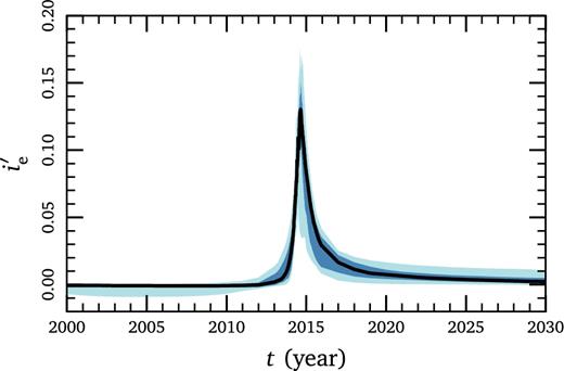
Eccentricity vector precession rate |$i_{\text{e}}^{\prime }=\boldsymbol {b}\cdot \boldsymbol {e}^{\prime }$| in radians per year (see equation A4) for models with inflow. It is strongly peaked at pericentre, justifying the impulse approximation described here. Shaded regions indicate 1σ and 2σ quantiles.
The orbit vectors |$\boldsymbol {j}$| and |$\boldsymbol {e}$| are constant in a Keplerian potential, but evolve in response to a non-Keplerian force. Measuring time evolution in the magnitude or direction of |$\boldsymbol {j}$| and |$\boldsymbol {e}$| thus directly relates to components of the non-Keplerian force.
APPENDIX B: ACCRETION FLOW PARAMETERS
Fig. B1 shows the probability distributions for the parameters in our MCMC model. Our results are as follows.
The rotation axis of the accretion flow, described in polar (θ) and azimuthal (ϕ) coordinates,8 is essentially unchanged from what we found in MM16, θ ∼ (105 ± 16)° and ϕ ∼ (−51 ± 23)°. In Kepler coordinates (as defined in Lu et al. 2009), our best-fitting accretion flow axis corresponds to (i, Ω) = (75° ± 16°, 51° ± 23°). For reference, we show the Galactic rotation axis in orange and the circumnuclear disc axis in green. This result depends on the perpendicular torque |$\boldsymbol {\tau }_{\perp }$|, which results from forces out of the orbital plane. This prediction is therefore relatively insensitive to radial inflow or outflow in the model.
We find a marginal detection of inflow of the accretion flow, with frad < 0. With our simplified model for the background, the data do not allow outflow along the orbit trajectory. The magnitude of the inflow parameter, |frad|, is degenerate with the size and shape of the cloud. The rotation parameter fkep approximately fixes |$\boldsymbol {\tau }_{\perp }$|, while the inflow parameter frad influences fr. Since both fr and |$\boldsymbol {\tau }_{\perp }$| are fixed with the data, the parameters are fkep and frad approximately linearly degenerate.
Since G2 has a nearly radial orbit, inflow reduces the Mach number of the cloud relative to its background. This significantly weakens our constraint on the strength of the magnetic field. While MM16 found a tight relationship between the field strength β and by density α, we find very low field strengths (β ≫ 1) are allowed if the inflow velocity is well matched to G2's velocity (frad ∼ −1). This is exacerbated by the simplicity of our model, in which all velocities scale exactly |$\propto \sqrt{G M_{\bullet }/r}$|.
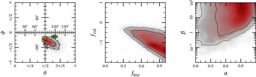
Probability distribution functions of the parameters in our model, determined using a maximum-likelihood analysis. Lines indicate 1σ and 2σ quantiles from the best-fitting solution. Left: the rotation axis of the accretion flow in polar angle, θ, and azimuthal angle, ϕ. As a comparison, we overplot the rotation axis of the Galaxy (orange) and that of the circumnuclear disc (green). Middle: the parameters frad and fkep which describe the strength of the inflow and rotation velocity of the accretion flow relative to the local circular Kepler velocity. Negative frad indicates an inflow solution. Right: the slope of the density profile of the accretion flow, α and the magnetic β of the plasma are strongly degenerate with respect to one another as both control the magnitude of the drag force.
APPENDIX C: KEPLER ELEMENTS
In Fig. C1, we plot the time evolution of the Kepler elements. Blue curves show the evolution in models with inflow; yellow curves show those without inflow from MM16. The top panels show eccentricity and semimajor axis of the best-fitting trajectories. Models with inflow result in less energy evolution before pericentre than in models without, because inflow reduces the relative velocity of the cloud with respect to the background. As the change in angular momentum is the same in both models, both semimajor axis and eccentricity evolve more slowly. The bottom panels show the change in orbital plane with time. Models with and without inflow show similar evolution. This is to be expected as changes in (i, Ω) are driven by the component of the force out of the orbital plane |$\boldsymbol {f}_{\!\text{j}}$|. Including a radial component |$\boldsymbol {f}_{\!\text{r}}$| in our model does not directly affect this. In contrast, the evolution in the angle of pericentre ω is very different in models with and without inflow (see top panel of Fig. 2). This is due to precession of the eccentricity vector.
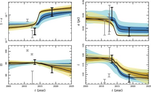
Time evolution of the Kepler elements in models with (blue) and without (yellow) inflow. Shaded regions indicate 1σ and 2σ quantiles. Observational estimates for G1 and G2 are shown with error bars (G1 estimates are placed 12.8 yr in advance of G2's as we treat their orbits as a single trajectory). In black, we show those derived from the same Br-γ data set used in our fits (Gillessen et al. 2013a,b; Pfuhl et al. 2015); in grey are those derived from the L΄ data (Phifer et al. 2013). We note that these data are slightly inconsistent. The top panels show evolution in eccentricity e and semimajor axis a. There is less energy evolution in models with inflow; both a and e decrease less in these models than those without inflow. The middle panels show the evolution in the orbital plane (i, Ω). Models with and without inflow evolve similarly as this is determined by the component of the force out of the orbital plane |$\boldsymbol {f}_{\!\text{j}}$|.
We also plot the derived Kepler elements for G1 and G2. In black, we show those derived from the same Br-γ data set used in our fits (Gillessen et al. 2013a,b; Pfuhl et al. 2015); in grey are those derived from the L΄ data (Phifer et al. 2013). We note that comparing Kepler elements is a very indirect comparison. If G1 and G2 are indeed gas clouds, their path is evolving on a time-scale much less than an orbital period. Fitting Kepler elements to the data, while instructive, does not provide an accurate test for theoretical modelling.
