Wide- and contact-binary formation in substructured young stellar clusters

Dorval, J.; Boily, C. M.; Moraux, E.; Roos, O.

doi:10.1093/mnras/stw2880

Abstract

We explore with collisional gravitational N-body models the evolution of binary stars in initially fragmented and globally subvirial clusters of stars. Binaries are inserted in the (initially) clumpy configurations so as to match the observed distributions of the field-binary-stars’ semimajor axes a and binary fraction versus primary mass. The dissolution rate of wide binaries is very high at the start of the simulations, and is much reduced once the clumps are eroded by the global infall. The transition between the two regimes is sharper as the number of stars N is increased, from N = 1.5 k up to 80 k. The fraction of dissolved binary stars increases only mildly with N, from ≈15 per cent to ≈25 per cent for the same range in N. We repeated the calculation for two initial system mean number densities of 6 per pc³ (low) and 400 per pc³ (high). We found that the longer free-fall time of the low-density runs allows for prolonged binary–binary interactions inside clumps and the formation of very tight (a ≈ 0.01 au) binaries by exchange collisions. This is an indication that the statistics of such compact binaries bear a direct link to their environment at birth. We also explore the formation of wide (a ≳ 5 × 10⁴ au) binaries and find a low (≈0.01 per cent) fraction mildly bound to the central star cluster. The high-precision astrometric mission Gaia could identify them as outflowing shells or streams.

methods: numerical

1 INTRODUCTION

The properties of stellar populations at birth hold a key to their long-term evolution as clusters or associations. Whether a stellar system will remain bound or undergo rapid dissolution hinges on the global star formation efficiency, the phase-space statistics of the stars, and the demographics of the type of stars involved (single or multiple; see e.g. Portegies Zwart, McMillan & Gieles 2010 for a synthetic review). The properties of binary stars in dense stellar associations in particular may shed light on the discovery of multiple star-formation episodes in rich stellar clusters (Anderson et al. 2009). For instance, binary stars enhance strong dynamical interactions which in turn may speed-up evolution off the main sequence and thus boost enrichment of the interstellar medium through winds (e.g. Tailo et al. 2015). Tight binaries of short-lived massive stars may evolve to produce exotic stellar remnants including black hole progenitors (Bacon, Sigurdsson & Davies 1996; Davies et al. 2009).

That gravitational dynamics should play a role early-on in the life of a star cluster is often illustrated by comparison of a low-density environment of irregular geometry such as the Taurus Aurigae region, to the more symmetrically shaped and denser Orion Nebula Cluster (ONC, e.g. Da Rio, Tan & Jaehnig 2014). Another example comes from APO Galactic Evolution Experiment spectroscopic observations of NGC1333 showing that main-sequence stars have much larger velocity vectors than candidate stellar cores, a strong indication that the velocity field develops on the same Myr time-scale as star formation (Foster et al. 2015). Thus the assembly of a cluster as a whole may proceed over time in a hierarchical fashion, and undergo a phase of dynamical relaxation to virial equilibrium. The rapid, global merging of substructures would bring stars together at a different stage of their formation (as in NGC1333), while inducing a shift from a clumpy Taurus-like profile to a more regular one. A simple but important question is how the internal dynamics of such complex configurations may affect the characteristics of a population of binary stars.

Many authors have explored this question through optimized initial conditions (Kroupa & Burkert 2001; Marks & Kroupa 2012) or fractal configurations evolved with N-body integrators (Goodwin & Whitworth 2004; Allison et al. 2009; Parker, Goodwin & Allison 2011; Parker & Meyer 2014). A recurring feature of all these studies is that the binary fraction drops over time regardless of their components (masses), due, e.g., to close star–star encounters or heating from the external galactic tidal field (though in specific cases, such as supervirial substructured systems, the binary fraction may be constant, see e.g. Moeckel & Clarke 2011). Another common result is that large-separation, weakly bound binaries are preferentially destroyed during dynamical evolution. Vesperini & Chernoff (1996) explored the fate of binaries in violently relaxing uniform systems. Comparing the internal velocity dispersion of the pairs and that of the cluster, they showed their soft binaries were destroyed, though it had no significant impact on the global structure of the cluster.

Parker & Meyer (2014) pointed out that the distribution of semimajor axes a of the field population is a strong function of the primary's mass: at fixed a, low-mass binaries carry less binding energy so the distribution cuts off at shorter separation (∼20 au) than for binaries with a more massive primary (∼300 au). Their study of fractal initial conditions shows that gravitational dynamics enhances the dissolution of low-mass systems. This then provides a clue to account for the larger relative fraction of heavy stars in binaries, such as seen in a compilation by Raghavan et al. (2010).

We note that hydrodynamical calculations of star formation have found young heavy stars to be preferentially hosted in dense clumps (Maschberger et al. 2010). Furthermore, it is not clear yet whether binary populations should be tailored according to the system total mass because of the limited range of M ∼ 10² to ∼10³ M_⊙ of these studies (Kroupa & Burkert 2001; Parker et al. 2011; Parker & Meyer 2014). Recall that the intensity of the tidal field is a prime agent of binary heating. A trend with mass may be expected on the ground that the drive to equilibrium of more massive systems leads to deeper potential wells (e.g. Aarseth, Lin & Papaloizou 1988; Boily, Athanassoula & Kroupa 2002). A steep potential will give rise to strong tidal fields which may disrupt bound subsystems (Boily et al. 2004; Renaud, Gieles & Boily 2011). A definitive assessment of this effect is difficult to reach because the results are a strong function of the system's initial-mass distribution and kinetic-energy content (Boily et al. 2002; Caputo, de Vries & Portegies Zwart 2014).

In this contribution, we revisit this issue but through initial conditions built from the self-consistent Hubble–Lemaître (HL) fragmentation of a star cluster (Dorval et al. 2016). The clumpy mass profile has both a self-consistent velocity field and built-in mass segregation (more massive stars on average in more massive clumps). We ask how the characteristics of the binaries evolved from such models compared with those of the well-sampled field-binary population (Duquennoy & Mayor 1991; Raghavan et al. 2010). A basic expectation is that evolution of massive binaries in dense clumps will enhance mass segregation while boosting the dissolution of the wider binaries on a very short time-scale (e.g. Bacon et al. 1996; Aarseth 2003; Marks, Kroupa & Oh 2011).

In Sections 2 and 3, we recall the basic procedure to obtain initial conditions for stellar dynamics and how the binary population was created. We present our data sets and main results in Section 4. In Section 5, we discuss the formation of very tight binaries (separation a of the order of 10⁻² au) on a few Myr time-scale. We sum up our findings and address open questions in Section 6.

2 INITIAL CONDITIONS FROM HUBBLE–LEMAîTRE FRAGMENTATION

2.1 Initial setup

Dorval et al. (2016) pointed out that fragmentation modes of self-gravitation developed in expanding coordinates lead to substructured mass distributions that have characteristics similar to star-forming regions (i.e. fragments mass function, stellar contents). This ‘cosmological’ HL expansion phase is interpreted as global pressure support mimicking the action of turbulence and magnetic fields, which both delay the large-scale collapse of the self-bound system (e.g. Mac Low & Klessen 2004), yet allow for small-scale density enhancements to grow. A self-consistent fragmented state is reached when the expansion stops (Dorval et al. 2016; see Fig. 1). That configuration is then used as initial condition to explore the stellar dynamical evolution. The initial HL expansion parameter |${\cal H}_{\rm o} > 0,$| so the vector field is simply |$\boldsymbol {v} = {\cal H}_{\rm o} \boldsymbol {x}$|⁠, with the positions |$\boldsymbol {x}$| drawn from a uniform sphere. For the current work, we performed a large set of runs of HL fragmentation, listed in Table 1.

Figure 1.

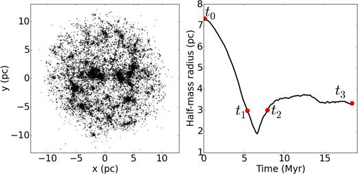
Left-hand panel: spatial distribution of a Hubble–Lemaître fragmented model. Right-hand panel: evolution of the half-mass radius over time. The times labelled as t₀–t₃ are the system configurations used in Section 4 for analysis. The model presented here is scaled for the lowest of the two initial stellar densities, 6 stars per pc³, has an initial half-mass radius of 7 pc, and is evolved up to 18 Myr. The denser model, starting with 400 stars per pc³, has the same aspect and evolution, with an initial half-mass radius of 1.8 pc and is evolved up to 2.3 Myr.

Open in new tab Download slide

Table 1.

Open in new tab

Summary of simulations. Starting from an HL fragmented configuration, a binary population was injected to complete the spontaneous binaries, reaching an overall binary fraction of 0.42. Densities within half-mass radius are shown at t = 0 and time of deepest collapse.

Name	N	Sampling	ρ_h,0 (pc⁻³)	ρ_h,max (pc⁻³)
R1.5h	1500	40	400	1.7 × 10³
R5h	5000	10	400	4.0 × 10³
R20h	20 000	10	400	1.4 × 10⁴
R80h	80 000	1	400	7.1 × 10⁴
R1.5l	1500	40	6	13
R5l	5000	10	6	79
R20l	20 000	10	6	192
R80l	80 000	1	6	10³

Name	N	Sampling	ρ_h,0 (pc⁻³)	ρ_h,max (pc⁻³)
R1.5h	1500	40	400	1.7 × 10³
R5h	5000	10	400	4.0 × 10³
R20h	20 000	10	400	1.4 × 10⁴
R80h	80 000	1	400	7.1 × 10⁴
R1.5l	1500	40	6	13
R5l	5000	10	6	79
R20l	20 000	10	6	192
R80l	80 000	1	6	10³

Table 1.

Open in new tab

Summary of simulations. Starting from an HL fragmented configuration, a binary population was injected to complete the spontaneous binaries, reaching an overall binary fraction of 0.42. Densities within half-mass radius are shown at t = 0 and time of deepest collapse.

Name	N	Sampling	ρ_h,0 (pc⁻³)	ρ_h,max (pc⁻³)
R1.5h	1500	40	400	1.7 × 10³
R5h	5000	10	400	4.0 × 10³
R20h	20 000	10	400	1.4 × 10⁴
R80h	80 000	1	400	7.1 × 10⁴
R1.5l	1500	40	6	13
R5l	5000	10	6	79
R20l	20 000	10	6	192
R80l	80 000	1	6	10³

Name	N	Sampling	ρ_h,0 (pc⁻³)	ρ_h,max (pc⁻³)
R1.5h	1500	40	400	1.7 × 10³
R5h	5000	10	400	4.0 × 10³
R20h	20 000	10	400	1.4 × 10⁴
R80h	80 000	1	400	7.1 × 10⁴
R1.5l	1500	40	6	13
R5l	5000	10	6	79
R20l	20 000	10	6	192
R80l	80 000	1	6	10³

2.2 Simulations

Each model was set up with stars drawn from the L₃ single star initial mass function (IMF) of Maschberger (2013). The L₃ IMF matches the better-known Kroupa (2001) and Chabrier (2003) functional forms but with fewer free parameters. We set a lower truncation mass of 0.1 M_⊙ and a maximum of 30 M_⊙, for an average mass of 0.5 M_⊙. This choice of truncation values allows us to take into account the impact of massive stars on the dynamics, while keeping the vast majority of stars on the main sequence for up to 18 Myr, the maximum simulation runtime. Simulations were therefore performed without stellar evolution. All phase-space coordinates were scaled to standard Hénon N-body computational units (Heggie 1975; Heggie & Mathieu 1986). In those units, G is set to unity, the total system energy E = −1/4, system mass M = 1, and global 1D velocity dispersion |$\sigma = 1/\sqrt{3}$| (exact for single-mass models). The initial velocity field of the HL fragmentation was set to |$\tilde{H}_{\rm o} = 1.2$| (dimensionless computational units). All simulations were run for t = 30 units of time.

The crossing time t_cr sets a reference time-scale with which to apprehend the state of the models. If we define r_h as the three-dimensional half-mass radius of a self-bound structure of internal velocity dispersion σ, its crossing time t_cr reads

\begin{equation} t_{\rm {cr}} \equiv \frac{2 r_{\rm h}}{\sigma }, \end{equation}

(1)

and the two-body relaxation time-scale, t_r, follows from (e.g. Meylan & Heggie 1997)

\begin{equation} \frac{t_{\rm r}}{t_{\rm {cr}}} \simeq \frac{0.138}{2} \left( \frac{r_{\rm h}}{r_{\rm g}}\right)^{1/2} \, \frac{N}{\ln (0.4N) }. \end{equation}

(2)

Here, r_g = 2 ≈ few × r_h is the gravitational radius of the structure of N stars. Importantly, these definitions apply equally to the system as a whole as to substructures inside it. This will be useful later, when we discuss the early evolution of binaries (Section 4). With equations (1) and (2), a cluster of N = 1.5 k single-mass stars has a relaxation time of ≈34 units. However, collisional effects of star–star interactions are much enhanced by the presence of a mass function. Then, the effective time for mass segregation, t_ms, scales roughly with 〈m〉/m_max × t_r ≃ t_r/60 for the current mass function. Therefore in such a small N = 1.5 k model, diffusion effect cannot be neglected over the course of the integration. We may reduce the impact of mass segregation by increasing N by a factor of ≈60 to N = 80 k. In doing so, we aim to catch the global dynamics more adequately, and highlight differences with systems that evolve collisionally throughout. We cover this range of membership from 1.5 k to 80 k with two intermediate values of 5 k and 20 k.

All integrations were done with the stellar dynamics code nbody6 (Aarseth 2003; Renaud et al. 2011; Nitadori & Aarseth 2012) for the efficient treatment of tight binaries. We analyse in the next section the population of binary stars in HL configurations before turning to their time evolution.

3 THE BINARY POPULATION

In this section, we first introduce our binary-detection algorithm. We then address the origin of spontaneous binaries, before adding ‘by hand’ a second population, with the aim to create a global population that recovers important characteristics of binaries (separations, binary fractions) observed in the galactic field.

3.1 Detecting the binaries

Binaries are detected as bound pairs satisfying a density criterion. For each star, the closest neighbours are found using a KD tree (Press et al. 2007), a data structure that allows neighbour searches with algorithmic complexity ∝log (N). Bound pairs are identified from the list of neighbours and the binary parameters derived for a subset of the pairs with the largest binding energy. The mean density of the two components, defined as

\begin{equation*} \rho _{\rm {binary}} \equiv \frac{m_1 + m_2 }{4\pi a^3/3 }\,, \end{equation*}

where a is the binary semimajor axis, is then compared to the local neighbour density obtained through the KD tree for 6–10 neighbours¹ (Casertano & Hut 1985). If the density ratio exceeds a threshold D,

\begin{equation} \frac{ \rho _{\rm {binary}} }{ \rho _{\rm {local}} } > D, \end{equation}

(3)

the pair is registered as a binary. If D is chosen too low, a lot of ephemeral binaries are found, while a high value picks only the closest binaries, ignoring wider, yet stable, systems. After testing with reference ensembles of binaries, we settled for D = 10 as yielding the best compromise. Other authors, e.g. Parker et al. (2009) and Lomax et al. (2015), have used close hybrids of the criteria that we have implemented.

Stars can be found to be part of several binaries at once, which happens more often for massive stars as they clear the density threshold more easily. When this happens, the algorithm selects from such connected systems only the pairs exhibiting the lowest (most negative) binding energy.

Star–star interactions which take place during the HL expansion phase speed up the internal evolution of small substructures (or clumps). The global expansion, on the other hand, brings about correlations in phase-space coordinates due to the predominantly radial motion of the stars. As a result, stars may pair up in the time-dependent potential if their mutual binding energy becomes negative (see Appendix A and Kouwenhoven et al. 2010; Moeckel & Clarke 2011 who discuss this in the context of dissolving clusters). We refer to this population as spontaneous binaries. There is a trade-off between the creation of spontaneous binaries during expansion, and their destruction/heating when they sit near or inside a clump. Wide binaries may survive for several internal periods if they form in low-density regions where the tidal field is weaker. Inspection of several simulations suggests that roughly 10 per cent of stars end up in wide binaries. Their properties as a subpopulation will be addressed statistically through numerical experiments.

In the analysis of the computer models, we refer to the binary fraction f_b as the ratio

\begin{equation*} f_{\rm b} \equiv \frac{ B }{ S + B} \end{equation*}

where S is the number of single stars, B the number of binary stars, and we will not consider multiple stars of higher rank (triples, quadruples, …: see e.g. Goodwin, Whitworth & Ward-Thomson 2004 and Hubber & Whitworth 2005 for a general extension to an arbitrary rank).

3.2 Spontaneous binary fraction versus primary mass

Several studies have found a strong correlation between the binary fraction f_m and the primary mass m of a binary system (for compilations, see e.g. fig. 17 of Bate 2012 and fig. 12 of Raghavan et al. 2010).² Since heavy stars tend to drive the formation of clumps in HL models, by attracting stars to themselves, it is natural to expect the HL procedure to give rise to a correlation of that nature.

The spontaneous binary fractions found in HL models for logarithmic primary-mass bins are plotted as light grey lines on Fig. 2. The shaded area shows the 1σ dispersion for these distributions. The fraction increases rapidly with primary mass, and is in close agreement with the data for primaries of mass higher than 2 M_⊙, when f_m exceeds 50 per cent. However, the HL models show a significant deficit of low-mass primary binaries in comparison to observational data.

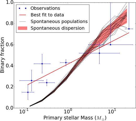
$Observational data of binary fractions (dots with uncertainties) as a function of primary mass. The data are taken in increasing primary mass from the following: Close et al. (2003); Basri & Reiners (2006); Fischer & Marcy (1992); Ward-Duong et al. (2015); Raghavan et al. (2010); Patience et al. (2002); Preibisch et al. (1999); Mason et al. (1998). The red line is a best-fitting linear relation. The thin curves and 1σ dispersion shaded area are the results for a population of spontaneous binaries obtained from HL models. The bins have a logarithmic width of about log(2).$

Figure 2.

Observational data of binary fractions (dots with uncertainties) as a function of primary mass. The data are taken in increasing primary mass from the following: Close et al. (2003); Basri & Reiners (2006); Fischer & Marcy (1992); Ward-Duong et al. (2015); Raghavan et al. (2010); Patience et al. (2002); Preibisch et al. (1999); Mason et al. (1998). The red line is a best-fitting linear relation. The thin curves and 1σ dispersion shaded area are the results for a population of spontaneous binaries obtained from HL models. The bins have a logarithmic width of about log(2).

Open in new tab Download slide

The high binary fraction for heavy primaries can be explained, at least in part, by considering the mass segregation occurring in the clumps during their formation. Dorval et al. (2016) have shown that massive stars tend to sink to the centre of clumps. These high-mass stars are more likely to capture another star to form a binary through a three-body interaction as they sit in denser environments (Spitzer 1987). A heavy star also creates a deeper potential well wherein to trap a fly-by star at the onset of HL fragmentation. There is indirect evidence for the three-body binary formation process to draw from mass-segregated clumps, because these binaries have a mean mass ratio q = m₂/m₁ that is significantly larger than expected from random pairing. The mean value of q for binaries with a primary star in the range 15–30 M_⊙ is indeed 0.21 ± 0.11, whereas random pairing yields a mass ratio of 0.02 ± 0.02 for that mass range. Due to mass segregation inside clumps, massive stars are more likely to pair up with moderately heavy companions rather than light ones.

3.3 Spontaneous semimajor axis distribution

The distributions of semimajor axes a and orbital periods are the main parameters used to characterize binary populations. Up to this point, the distances were given in computational N-body units. To convert the models to physical scales, we matched their stellar number density within the half-mass radius to that of observed clusters. King et al. (2012) compiled data for several young clusters and gave their stellar densities within half-mass radii, with high values reaching 400 stars per pc³, typical of the ONC, and low densities of ∼6 stars per pc³, more akin to the Taurus region. These are the two reference values used to build up our data set of numerical models. The time conversion gives a total duration of the simulations of 2.3 Myr for the high-density clusters and 18 Myr for the low-density ones.

In practice, the spontaneous binaries develop a bell-shaped distribution of separation centred on ∼2000 au for a high-density HL model, and ∼7000 au for a low-density one (see the broken curve on Fig. 4). This is much wider than the averaged value of ∼50 au for the Galactic field population (Duquennoy & Mayor 1991; Raghavan et al. 2010), where separations of ∼1 au or lower are not uncommon. It is none the less shorter than the 10⁴–10⁵ au peak found in N-body simulations of dissolving clusters (Kouwenhoven et al. 2010; Moeckel & Clarke 2011; see also the discussion in Appendix A).

Hydrodynamical calculations by Bate (2012) show that orbital energy dissipated in the early stages of formation may cause binaries with an ∼10 au separation to shrink to a ∼ 0.5 au in the course of t ∼ 1 Myr. Analytical arguments by Stahler (2010) and Korntreff, Kaczmarek & Pfalzner (2012) would have external drag forces from residual gas drive a tight binary to merge completely. Kroupa & Burkert (2001) have shown that stellar collisions alone cannot bring a narrow distribution of semimajor axes to the full width of observed values. Other authors, such as Parker & Meyer (2014) investigated the evolution of a binary population identical to the field but embedded in clumpy, fractal clusters (Goodwin & Whitworth 2004) to test the robustness of the field population, while Vesperini & Chernoff (1996) introduced binaries with a binding energy inverse power-law, favouring weakly bound pairs.

A full spectrum of separations is desirable for comparison with data and theoretical models but is not a natural outcome of the HL fragmentation.

A trick was used to add binaries to the fragmented HL initial conditions. We follow Parker & Meyer (2014) to ease comparison with their setup, by supplementing the population of spontaneous binaries with one that matches the field galactic populations at small a. In doing so, we should also constrain the statistical weights with mass so as to redress the deficit of small-mass primaries (Fig. 2).

3.4 Complete separation distribution: procedure

The addition of new binaries to the HL distribution is not straightforward, as the phase space coordinates of stars in an HL fragmented system are the consequence of the numerical evolution during the expansion (no known functional distribution function). A practical and coherent method builds the extra binary population before the HL expansion phase.

3.4.1 Binary parameter distributions

When introducing binaries in the system, primary masses are picked to account for the observed decrease in binary fraction with decreasing primary mass (see Fig. 2). Secondary masses are then randomly chosen in the remainder of the population. The resulting mass-ratio distribution is generally flat, slightly peaking at high mass ratios, mostly from low-mass stars paired with other low-mass stars. This has no bearing on our study, as the mass-ratio distribution has a negligible impact on the processing of a binary population (see Parker & Reggiani 2013).

Eccentricities are drawn from a flat distribution, which is consistent with observed populations; see section 5.1.4 of Duchêne & Kraus (2013). This distribution is not expected to be substantially affected over a few Myr of dynamical evolution (Kroupa 1995b) and evolves to a thermalized profile on a longer time-scale (e.g. Kroupa 2008).

Finally, binary separations and periods are drawn from Raghavan et al. (2010). To account for the excess of (spontaneous) binaries at large separations, a reduced statistical weight is used to lower their impact on the final distribution. For simplicity and to limit the number of parameters in this work, we chose to apply the same distribution of separations to all binaries. In future work, one would like to factor in the fact that observations show that the distribution changes with the primary mass (see Duchêne & Kraus 2013; Parker & Meyer 2014).

A binary is generated by a Monte Carlo method, then replaced by a point mass equal to the sum of its components, and the HL expansion carried out with a subset of such fused binaries. Once the system has fragmented, the fused binaries are split and their two components recovered along with their set internal parameters. The barycenter of the new binary follows the orbit of the original point mass.

There are drawbacks to the implementation of the method; the main ones are as follows: (1) The HL fragmentation develops with fewer stars than in the final system, after the splitting. Therefore, fewer spontaneous pairs may form than might have otherwise. (2) Some spontaneous pairs form at the end of the HL phase with one fused binary as a component. Many of these spontaneous binaries (we found ≈50 per cent) are no longer classified as bound pairs once the massive point mass is split into the binary. Thus, the value of a and the amplitude of the peak of the statistics for spontaneous binaries after the split is hard to fix or predict. These two caveats make the insertion of binaries a complex statistical process, which leaves some freedom in the final distribution at the characteristic scale of the spontaneous population (few 10³ au). Nevertheless, the final distribution comes close to the one sought, with differences (i.e. a relative excess of wide binaries) we may attribute to the formation history of the system.

3.4.2 Results for N = 20 k models

The procedure outlined in the previous subsection was tested on a set of 20 identical low-density models (≈6 stars per pc³; see Section 3.3) of 20 k stars. The resulting binary fraction is plotted on Fig. 3 as a function of the primary mass. The deficit of low-mass primaries was bridged, while the fraction for high-mass primaries was slightly reduced (from 0.85 down to 0.75 for a primary mass of ≈20 M_⊙; note the increased scatter). This is the effect mentioned in Section 3.4 of splitting fused spontaneous binary components with a heavy primary. (Several of these heavy spontaneous binaries with large separation no longer satisfy equation 3). A few massive binaries were introduced to compensate for this effect, which remains relatively small. The values derived for this range of primary masses remain in complete agreement with observational data. Extensive numerical exploration of binary tidal heating has been performed by one of us (Roos 2013). Binaries were put on highly eccentric orbits in cuspy Dehnen (1993) potentials, thus experiencing large variations in the tidal force. It was found that the binary binding energy varied by ≈50 per cent or more only when the semimajor axis a > 100 au. No binary–single stars or binary–binary interactions were included. The conclusion from this study is that binaries with axis a shorter than 100 au should rarely unbind due to tidal heating. Further tests with nbody6, and the results of the next section, largely confirm this. With that in mind, and in view of the computational costs, we truncated the binary population at a = 1 au. This choice allows us to recover the range found in the SPH calculations of Bate (2012), so a closer parallel can be made with his setup.

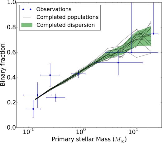
$Binary fraction as a function of primary mass. The results displayed are the average of 20 realizations for 20 k particles models; the shade indicates 1σ deviations. Short semimajor axis binaries were injected to complete the spontaneous population (compare with Fig. 2).The bins have a logarithmic width of about log(2).$

Figure 3.

Binary fraction as a function of primary mass. The results displayed are the average of 20 realizations for 20 k particles models; the shade indicates 1σ deviations. Short semimajor axis binaries were injected to complete the spontaneous population (compare with Fig. 2).The bins have a logarithmic width of about log(2).

Open in new tab Download slide

We show on Fig. 4 in short-dashed red the full spontaneous binary population (with a peak value at a ≈ 7000 au), prior to the procedure to split fused binaries. The distribution of separations for the fused binaries is shown as the long-dashed curve, with a dip around a ≈ 10 000 au. Finally, the splitting procedure is carried out, and the result shown as the solid curve. The grey shade is the expectation value for the parametrized Gaussian distribution of Raghavan et al. (2010). Discrepancies with this distribution are only significant for binaries with a > 4000 au. The peak of the spontaneous population, still visible after the splitting procedure, introduces an excess of binaries for (roughly) 4000 < a < 20 000 au. Note how the excess of binaries in that range has been halved by the splitting procedure, dropping from a maximum of ≈370 to ≈170. For separations larger than a > 10⁶ au, the binaries are not identified by the density threshold algorithm and are dropped from consideration. Since none of them are likely to survive for a long period of time given the density of the system, this will have no bearing on our conclusions.

Figure 4.

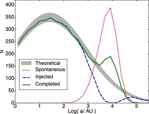
Distribution of binary separations for the completion of a population in a low-density model. Spontaneous binaries before splitting are shown in short-dashed red, the population injected in the system in long-dashed blue, and the resulting measured distribution in the completed system in green. The observational separation distribution from Raghavan et al. (2010) is shown as a grey area, taking into account Poisson dispersion.

Open in new tab Download slide

4 EVOLUTION OF BINARY POPULATIONS

A system bound gravitationally will resist external tidal forces if it sits within its Roche radius (Binney & Tremaine 2008, section 8; Renaud et al. 2011). For binary stars, the condition for boundedness is given by equation (3) with D = 3 and setting the mean density ρ_bin over the full Jacobi volume. Thus, the question of how much the mean background density rises and compares to the mean density of the binary has important consequences for the further evolution of the binary. The situation is made more complicated if the host's potential changes rapidly, on the dynamical time-scale t_cr of equation (1).

Let us first recall the results of the collapse of a homogeneous sphere of N identical stars. In this case, the sphere collapses by a factor C before it rebounds and evolves towards equilibrium (Aarseth et al. 1988; Boily et al. 2002). The ratio of minimum radius achieved during collapse, to the initial system radius, is a 1/3 power-law of N, so C ∝ N^−1/3. If the total mass is conserved during the collapse, the mean background density scales as ρ ∝ C⁻³ and so reaches a peak value max (ρ) ∝ N. Based on this analysis, one would expect a strong relation between the system total mass |$M = N \overline{m}$| and the rate of destruction of binary stars, especially those of large semimajor axis a, if and when a cluster undergoes a phase of collapse.

Various simulations were performed: their parameters are summarized in Table 1. Runs with N ranging from 1500 to 80 000 were sampled in such a way that ensemble-averaging gave roughly the same Poissonian standard deviations in each case.

4.1 Results

We show on Fig. 5 the evolution of the binary fraction in HL fragmented systems as a function of time. The time when the systems rebound from the global infall, t ≈ 10 units, is marked with a vertical dotted line on each frame. The binary fraction decays in each case during the course of evolution, regardless of their membership N or initial density. All systems display two different regimes of binary destruction, before and after the bounce from global collapse. Before the bounce, binaries are destroyed at a higher average rate, more so for the more massive systems (large N). After the bounce (t > 10), the slopes all flatten out and binaries are continuously destroyed, but at a lower rate. For example, the high-density N = 80 k simulation removes 2.5 per cent of its binaries per time unit before the collapse; this rate goes down to 0.25 per cent afterwards. Similarly, the low-density N = 80 k run has 1.7 per cent before the collapse and 0.16 per cent thereafter.

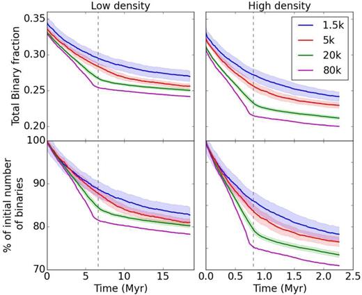
$Top panels: total binary fraction over time for different cluster memberships. Lower panels: total number of binary over time compared to initial number in each system, in percentage. The vertical dashed line indicates the time of deepest collapse.$

Figure 5.

Top panels: total binary fraction over time for different cluster memberships. Lower panels: total number of binary over time compared to initial number in each system, in percentage. The vertical dashed line indicates the time of deepest collapse.

Open in new tab Download slide

We interpret these findings as follows. In the first stages of evolution, the rate of binary destruction is driven by the two-body relaxation in the small clumps of the HL configuration. To see this, Fig. 5, bottom row, graphs the relative fraction of surviving binaries for each model. The linear slope is virtually identical up to t ≈ 5 units. The internal dynamics of clumps is independent of the larger system in which they are embedded. As collapse proceeds, larger N systems develop a deeper global potential well: this is easier to see for t → 10 as the curves fan out. The range, of about 10 per cent, accrued at t = 10 between runs of different N, is almost unchanged at the end of the simulations, at t = 30 units. The rate of binary destruction post-bounce is practically the same for all N, though note that it remains higher for the high-density calculations (the final count of binaries drops from ≃80 per cent at low density to ≃70 per cent at high density).

There is a clear tendency for the pre- and post-collapse transition to be sharper as N increases. We interpret this in the light of equations (1) and (2). We note that the N = 1.5 k models are dominated by two-body interactions, when the mass-segregation time-scale drops to ∼1 time units, and not by the overall collapse motion that drives density upwards, destroying binaries. At the other end of the spectrum, the N = 80 k models have a global mass-segregation time-scale >30 time units. These models, like all the others, are initially dominated by two-body interactions in their clumpy substructures. However, the later evolution sees the overall collapse motion take over. It is the imprint of that global infall which allows the density to peak at higher values (cf. Table 1) and laminate binaries more efficiently around that time. Since the rebound is of short duration, the strong tidal field drops quickly as we shift in the post-bounce phase.

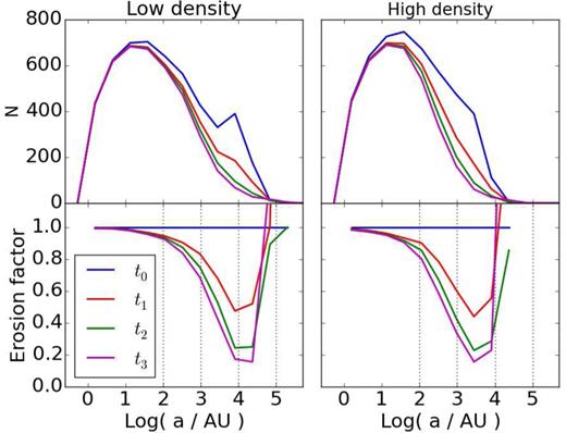
To determine whether the evolution affects binaries differently according to their mass, we show on Figs 6 and 7 the binary fraction in relation to the primary mass. Results are shown at four different times, and for all runs of N. The top row of each figure is the binary fraction f_m and the bottom row the percentage of binaries with respect to the initial distribution.

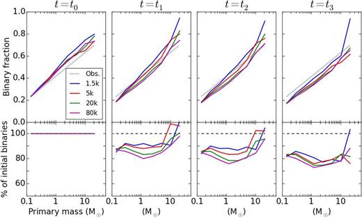
$Top panels: the binary fraction in logarithmic bins for the primary masses. The dotted line is the linear fit to observations shown on Fig. 2. Bottom panels: the number of binaries in each primary-mass bin is shown as a percentage of the initial number (t = 0). The horizontal dashed line is 100 per cent. The data are from low-density models.$

Figure 6.

Top panels: the binary fraction in logarithmic bins for the primary masses. The dotted line is the linear fit to observations shown on Fig. 2. Bottom panels: the number of binaries in each primary-mass bin is shown as a percentage of the initial number (t = 0). The horizontal dashed line is 100 per cent. The data are from low-density models.

Open in new tab Download slide

Figure 7.

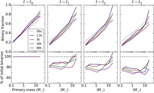
Same key as Fig. 6. The data are from high-density models.

Open in new tab Download slide

This representation highlights which binaries are the most processed in the system. The panels for t = t₁ and t₂ are for times immediately before and after the bounce (cf. Fig. 1). The dynamical evolution within the clumps and during the collapse impacts preferentially light-primary binaries; binaries with a more massive primary (say, >5 M_⊙) survive better. We stress that the trends are indicative and at the ∼20 per cent level in all cases. Bearing this caveat in mind, inspection of the different cases does suggest that the results for low-N runs are more the result of the internal dynamics of clumps, where star–star interactions would favour the ejection/destruction of low-mass binaries. Note how the low-N models in fact form additional high-mass binaries during infall, since the binary fraction exceeds 100 per cent at t = t₁ and t₂. This is not so for the N = 20 k and 80 k models, which we interpret as being due to the stronger tidal fields in these models which stops new binaries from forming. It is interesting that despite the deeper infall achieved by these large-N models, the trend of increased survival with primary mass is not eradicated: this would have been the case had the external (global) tidal field clearly dominated the binary destruction. Instead, we find that the strong fields do not erase memory of the early evolution phase of the clumpy distribution.

The results for the later time t = t₃ displayed coincides with the end-time of the simulations. At that point, all models have reached equilibrium and the binaries have been processed dynamically in such a way that the binary fraction decreased monotonically for all primary masses. It is worth noting that the low-density models (Fig. 6) have evolved for a physical time t ≈ 18 Myr, while the high-density ones (Fig. 7) up to t ≈ 3 Myr only. This may explain the greater scatter among the different runs for these models (they have more intense tidal fields but have less time to act on the binaries). We also note that the peak at high primary mass, clearly visible at t = t₂, is still apparent at t = t₃, except for the case N = 80 k, which is the model with the highest density and the strongest tidal field. We interpret this as indicating that the wide binaries have had time to be split, while this process is yet incomplete in the other models. This view is backed up from inspection of the low-density runs at t = t₃ on Fig. 6, where all the peaks seen at t = t₂ have been flattened, save the runs with N = 1.5 k. We believe that the more stochastic low-N runs may have produced more wide-binary escapers due to their shallower potential well. These would therefore not be processed collisionally in the final cluster and survive in isolation.

4.2 Semimajor axis distributions

The evolution of the distribution of semimajor axes a in a binary population hinges on its dynamical environment. Several analytical and numerical studies (Heggie 1975; Kroupa 1995a,c; Vesperini & Chernoff 1996; Heggie, Trenti & Hut 2006; Parker et al. 2009, 2011) have shown that wide, weakly bound binaries are preferentially disrupted, thus sculpting the distribution towards tighter, more bound binaries. This evolution is shown on Fig. 8, which graphs the distribution histograms as a function of semimajor axis a. The distributions are plotted for four various times, membership N and both the values of initial density. The averaged distribution computed from the models with N = 1.5 k is shown as a dotted line and serves as reference. To ease the comparison between models with different N, all histograms were normalized to the reference initial profile at t = 0 (e.g. the area under the curve is the same for all the models).

Figure 8.

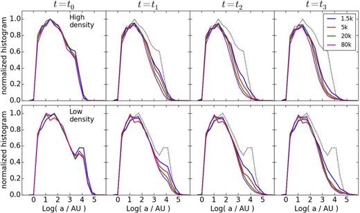
Histograms of semimajor axes for the binary population at four different times and for four different cluster membership. The dotted black line shows the distribution of N = 1.5 k models at t = 0 as a reference for the initial distributions. High-density models are in the top row, while low-density models are in the bottom row. The reference times are taken from Fig. 1.

Open in new tab Download slide

We first distinguish between high- and low-density models. The overall behaviour of the models is the same, with a rapid dissolution of large semimajor axis binaries, a ∼ 10³ au or more. This takes place prior to the bounce, when t < t₁, but is a continued trend from the start of the computations to the end. As anticipated, high-density models (top row on Fig. 8) process the binary population more efficiently, reaching deeper in the short-axis range, down to a ∼ 20 au, compared to a ∼ 100 au for the low-density models. This can be gauged qualitatively by the gap that opens up between the dotted line and the histograms.

The system mass (or membership N) has little influence on the evolution of the histograms; however, as the collapse factor C increases with N, the larger N models process significantly wider a ∼ 10³ au binaries; this is true regardless of the initial density (high or low). Note that, here too, the N = 1.5 k models stand out, in the sense that their wide binary population is less efficiently processed.

Having identified the mean initial density as the main driver for binary population evolution, we wish to quantify the rate of survival of binaries. We define the erosion factor as the ratio, in each semimajor axis bin, of the current number of binaries to the initial population. This allows us to asses easily the processing power of the system at all separations. The idea was borrowed from Marks et al. (2011) and Marks & Kroupa (2012) who introduced an analytic operator acting on a binary population to mimic its evolution in a host star cluster. The erosion factor is bound to the interval [0, 1], and equals 1 when all binaries of a given semimajor axis a are retained (zero when they are all destroyed).

We measure the quantities of binaries in separation bins over time to define the erosion factor for our simulations. It is displayed for the four reference times and for N = 20 k simulations on Fig. 9 (bottom panels). The model with initially high density heats up and splits binaries of (relatively) shorter semimajor axis during the collapse, and beyond: the most dramatic phase of evolution between times t₀ and t₂. During that interval, nearly 80 per cent of binaries with a > 1000 au are split. There is comparatively little evolution from t₂ to t₃, which covers the remaining half of the runtime. The run of the erosion factor with a and its time-evolution are very similar when comparing the runs of models with high- and low initial density. The most striking difference is the shift of the minimum value of the erosion factor, from a semimajor axis a ≈ 3000 au, to larger axes a ≈ 10 000 au in the case of low-density models. The extent of the shift, a factor of 4, is consistent with the scaling of the mean separations between stars l ∝ ρ^−1/3; we compute for high- and low-density systems

\begin{equation} \frac{l_{\rm {low}}}{l_{\rm {high}}} = \left( \frac{\rho _{\rm {high}}}{\rho _{\rm {low}}}\right)^{1/3} = \root 3 \of {\frac{400}{6}} \simeq 4. \end{equation}

(4)

Figure 9.

Top panels: histogram of semimajor axis at four different times for the N = 20 k models. Bottom panels show the erosion factor, the ratio between the sizes of the initial binary population and the one at a given time, in each primary-mass bin.

Open in new tab Download slide

This fact alone implies that the evolution of fragmented mass profiles through a relaxation phase is driven mostly by stellar encounters. The same conclusion applies for the evolution of the fractal models of Parker et al. (2011).

4.3 Tidal shocks

We noted how larger N simulations tend to iron out a larger fraction of binaries (see Fig. 8). The weak trend with increasing N implies that both star–star interactions (including multiple stars) and global tidal forces both boost the heating up and unbinding of binaries. The shift seen on Fig. 7 is small but systematic: from 15 per cent for N = 1.5 k to 25 per cent for N = 80 k of all binary stars are destroyed at the bounce (t ≈ 10 units). To get a better appreciation for the trend (or lack thereof) with N, let us compute the energy transferred to a binary star by the tidal field. At the end of the collapse, the stars move on mostly radial orbits at high velocities. Since they cross a dense region in a short time, we make use of the tidal shock approximation developed by Spitzer (1958, see also Boily et al. 2004; Binney & Tremaine 2008, section 8).

Taking inspiration from the tidal shock suffered by a cluster crossing the galactic disc, we can get an estimation of tidal heating on a binary crossing the dense centre of the system at the time of deepest collapse. Binney & Tremaine (2008) define the change of specific binding energy ΔE_s of a self-gravitating system of size a, mass μ, crossing a spherical volume of projected surface density Σ ≈ rρ at radial velocity V_r, as

\begin{equation} \Delta E_{\rm s} = \frac{14 \pi ^2 G^2 \Sigma ^2 a^2}{3 V_{\rm r}^2}\,. \end{equation}

(5)

We seek out the scaling of this relation with the number of stars N, keeping the system's initial mean density ρ(0) constant. This implies that the total mass M ∝ N. The expectation from the analysis of fragmentation modes is that the radius at the bounce r = R_o/N^1/3. The projected density at the bounce therefore scales as Σ ≈ M/πr². Ignoring mass-loss and the energy dissipated by binary disruption, we can estimate the magnitude of the square radial velocity |$V_{\rm r}^2$| from the relation

\begin{equation} 3 V_{\rm r}^2 \approx \frac{2G M}{r} \propto \frac{N}{N^{-1/3} R_{\rm o}}. \end{equation}

(6)

Substituting in (5) and replacing r by the semimajor axis a, we find

\begin{equation} \Delta E_{\rm s} = \frac{14\pi G^2(M / \pi r^2)^2 a^2}{ 2GM / r } \propto \frac{G M \, a^2}{r^3} \propto \frac{GM}{R_{\rm o}^3} N a^2\,. \end{equation}

(7)

The binding energy per unit mass of a binary star is E_s = −Gμ/2a. The relative energy imparted to the binary by the shock is therefore

\begin{equation} \frac{\Delta E_{\rm s} }{E_{\rm s}} \approx \frac{7\pi M}{\mu R_{\rm o}^3} a^3 N \,. \end{equation}

(8)

We chose to keep the initial mean system density constant, so that the ratio |$M/( \mu R_{\rm o}^3)$| is independent of N. The final scaling reads

\begin{equation} \frac{\Delta E_{\rm s}}{E_{\rm s}} \propto a^3 N \,. \end{equation}

(9)

An increase in membership N implies more significant heating of the binary star. If we set ΔE_s/E_s = 1, then an increase of N → 10 × N should have the same relative effect on a binary of semimajor axis a → a/10^1/3 ≈ a/2.15. By implication, the peak of the distributions seen on Fig. 8 should shift from a ≈ 40 au to a ≈ 40/3.76 = 10.64 au, as we work up from N = 1.5 k to 80 k calculations. This shift is not seen on the figure. What we see, on the other hand, is that large-N systems tend to deplete more efficiently the wide binaries, so that at the same stage of evolution, the richer systems have a binary distribution that falls off more quickly at large separations. We attribute the weak dependence on N to the approximation of a static background mass distribution.³ In reality, the whole structure moves on the same short dynamical time-scale of equation (1) and hence the effective surface density Σ is much reduced if the system as a whole begins to re-expand. We suspected that the choice of fixed initial density may be the reason for the undetectable shift of the peak on Fig. 8. Our choice of initial conditions implies that the system size R_o ∝ M^1/3; had we chose instead to use an empirical relation such as R_o ∝ M^1/5 for stellar clusters (Larsen 2004), we would have found a scaling of ΔE_s/E_s ∝ a³N^7/5. The same rise in N as before would have produced a shift from ≈40 to 6.5 au in the peak of the distribution, and this is still too large to go undetected.

5 EXTREME TIGHT AND WIDE BINARIES

As mentioned in Section 3.2, Bate (2012) has found several examples of binaries reducing their separation over time through stellar encounters, from ∼10 au down to ≲0.5 au. Tighter systems were hindered by numerical resolution issues. The regularized treatment of close encounters (which allows us to integrate up to machine precision) of the code nbody6 means that the same collisional process will be at play in the calculations that we have performed. Since no binaries with semimajor axis a shorter than 1 au were inserted in the initial conditions, we focus first on the statistics of binaries that evolved to a < 1 au. In the second part of this section, we will explore the formation and the evolution of very wide (a > 10⁴ au) binaries, many of which end up loosely bound to the stellar cluster as a whole.

5.1 Tight binaries

Several binaries with a < 1 au were detected at the end of the low-density simulations. By comparison, almost none developed in the high-density runs. Their properties are summarized in the left-hand panel of Fig. 10. The data are taken from N = 20 k runs but similar statistics were obtained for the other setups. The top row shows the binary's mass as a function of semimajor axis, while the bottom row on that figure graphs the distance of their barycentre to the centre of the cluster. Open circles denote binaries that already existed at t = 0, and became tighter over time, while filled circles are new binaries that formed in the course of the simulation. Inspection of these new, tight binaries shows that both of their components were part of binaries originally inserted in the system. Thus all new tight binaries shown on Fig. 10 are the results of strong binary–binary interactions leading to splitting or exchange. (None of the original binaries that survived to the end of the simulation had a < 1/2 au.)

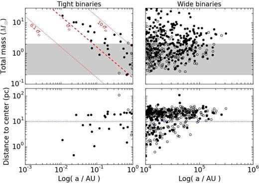
$Left-hand panels: total binary mass (top) and distance to centre of the cluster (bottom) versus the semimajor axis for binaries tighter than 1 au at the end of the simulation. Right-hand panels: same layout for binaries wider than 104 au. The greyed area in the top panels shows the 90 per cent probability range of a binary total mass from random pairing given the present IMF. The red dashed line in the top-left panel shows the relation for constant $v^2_\infty \sigma _{\rm {coll}} \equiv \sigma _0$; it is bounded by two dotted curves that have 10σ0 (above) and 0.1σ0 (below). The horizontal dotted line in the bottom panel indicates the boundary between the ejecta (distance to centre >10 pc) and the central system. Open circles are binaries which already existed at t = 0. The data are from 10 simulations of N = 20 k stars with initial mean density of 6 per pc3.$

Figure 10.

Left-hand panels: total binary mass (top) and distance to centre of the cluster (bottom) versus the semimajor axis for binaries tighter than 1 au at the end of the simulation. Right-hand panels: same layout for binaries wider than 10⁴ au. The greyed area in the top panels shows the 90 per cent probability range of a binary total mass from random pairing given the present IMF. The red dashed line in the top-left panel shows the relation for constant |$v^2_\infty \sigma _{\rm {coll}} \equiv \sigma _0$|⁠; it is bounded by two dotted curves that have 10σ₀ (above) and 0.1σ₀ (below). The horizontal dotted line in the bottom panel indicates the boundary between the ejecta (distance to centre >10 pc) and the central system. Open circles are binaries which already existed at t = 0. The data are from 10 simulations of N = 20 k stars with initial mean density of 6 per pc³.

Open in new tab Download slide

The statistics of these events should be compared with expectations based on estimated collision rates. The time-scale for direct collisions between particles in a self-gravitating system depends on the degree of gravitational focusing of the colliding bodies (Binney & Tremaine 2008, section 7.5.8, equation 7.195a). This is given quantitatively by the Safronov number |$\Theta = v_\star ^2/4\sigma ^2 = G M / (4\sigma ^2 a)$|⁠, where we have replaced the surface escape velocity v_⋆ of a single star by the unbinding velocity v² = GM/a of a binary of total mass M and separation a. To obtain an estimate of Θ, we looked at typical clump parameters from the N = 20 k R20l models: an average membership of N_c ∼ 50 stars and mean half-mass radius r_h ∼ 0.2 pc yield an internal velocity dispersion (subtracting the binaries’ internal motion) σ ∼ 0.5 km s⁻¹. Setting a binary mass M > 2 M_⊙ and semimajor axis a = 1 au yields Θ ≃ 3700 ≫ 1. The collisional rate |$\tau _{\rm {coll}}^{-1}$| for binary disruption is then

\begin{eqnarray} \tau _{\rm {coll}}^{-1} &=& 16 \sqrt{\pi } n \sigma a^2 \Theta \nonumber \\ &=& 8\times 10^{-4} {\rm \,Myr}^{-1} \frac{n}{700\, {\rm pc}^{-3}} \frac{0.5\, {\rm km\,s}^{-1}}{\sigma } \frac{a}{{\rm au}} \frac{M}{2\, {\rm M}_{\odot }} \end{eqnarray}

(10)

with n the stellar number density ∼700 pc⁻³. This rough estimate of the collision rate should be interpreted as a lower limit because in practice a > 1 au and many binaries have a total mass >2 M_⊙. We find |$\tau _{\rm {coll}}^{-1} \sim 8\times 10^{-4}$| collisions per clump per Myr. Since on average ≃ 150 clumps are formed in each R20l run, and assuming that the collision rate is constant throughout the 6 Myr infall time, we expect hard encounters of order O(1) per 10⁴ stars. If most of these interactions lead to the disruption of the binaries, some others will result in exchange and tighter components.

These statistics are in good agreement with the identification in the 10 N = 20 k runs of a total of 24 binaries with a < 0.6 au, for an average of 2.4/5000 ≈ 0.05 per cent of all binary stars (f_b ≈ 1/3 at t = 0). The very tight binaries each have a combined mass exceeding 2 M_⊙ with a low mass ratio q, ranging from 0.01 up to 0.2. It is important to mention that main-sequence binary stars with a separation a ≲ 0.02 au would be contact binaries when both members are solar-type or more massive stars. Clearly the evolution of such objects (and in fact their formation process) calls for hydrodynamical effects that were not included in our study. It is therefore remarkable that contact binaries should form strictly through gravitational scattering on such short time-scales.

These results apply to runs with initial mean number density of 6 per pc³. The same analysis carried out for the higher density models give a different outcome. For these models, the initial density is larger by a factor ∼60 and the velocity dispersion by a factor ∼2, for all stars. From equation (11), we find a collisional rate ∼30 times higher than previously. If direct collisions were the main channel for the formation of tight binaries, the number of events should increase in the same proportions. However, inspection of the simulations yielded only four tight binaries, each with a semimajor axis a ≳ 0.1 au. Thus the rate of formation of tight binaries drops to 0.4 per 5000 binaries, or 0.008 per cent, a six-fold decrease. We argue that two factors hinder the formation of these objects in high-density environment. First, Geller & Leigh (2015) pointed out that exchange encounters between single stars and binaries are not instantaneous (see also Hut & Bahcall 1983). The process can be perturbed by other stars, so modifying the outcome of the collisions. This is also true for binary–binary collisions: casual inspection of the time series of (tight) binary stars showed that their mean separation keeps evolving throughout the evolution of the model, which suggests that the binaries are part of a small-N hierarchical system. It is reasonable to expect that more hierarchical systems will develop in a higher density environment (involving more stars) and so the exchange process may never have time to take place.

Secondly, the binary exchange cross-section is sensitive to the impact velocity. The lack of a detailed theoretical framework on binary–binary collisions makes it difficult to pin down statistical expectations with precision. In the case of a disruptive encounter between a binary + single stars, extensive analytical work by Mikkola (1983, 1984a,b) and numerical scattering experiments (e.g. Heggie, Hut & McMillan 1996; Fregeau et al. 2004) lead to a rough estimate of the effective scattering cross-section σ_coll in relation to the mass and separation of identical binaries:

\begin{equation} \sigma _{\rm {coll}} \propto \frac{m_t a}{v_\infty ^2}\,. \end{equation}

(11)

In this equation, σ_coll is the effective collisional cross-section for disruption in binary–single interactions, and v_∞ is the relative velocity at infinity (prior to the collision) ≈ the clump velocity dispersion. Taking v_∞ ≈ σ = constant independent of mass and binary separation, we may use equation (11) to relate binary mass M to separation a and cross-section σ_coll. Hut & Bahcall (1983) and Hut (1983) gave analytical expressions for the exchange cross-sections, which scales as the above scattering cross-section at low velocities, but becomes steeper for higher velocities:

\begin{equation} \sigma _{\rm {ex}} \propto \frac{m_t a}{v_\infty ^6}\,. \end{equation}

(12)

As the encounter velocity increases, it becomes harder and harder to perform a successful exchange. The two initial mean densities that we picked may therefore cover the transition from low- to high-velocity regimes, and reduce the number of tight binaries created to just a handful.

Going back to Fig. 10, we plot the relation |$v^2_\infty\, \sigma _{\rm {coll}} \equiv \sigma _0$| of equation (11) as straight red lines on the top-left panel. Two dashed curves bracket a curve in full type, each with a value of σ_coll differing by a multiplicative factor of 10 (increasing from the lower curve, up). The large separations between the curves and the clustering of data points along the dashed curve indicate how a single value of σ₀ effectively cuts through the diagram in two well-delimited regions. Thus, the trend of binary mass increasing as M ∝ 1/a for the most tight binaries is consistent with a constant product of |$\sigma _0 = v^2_\infty \sigma _{\rm {coll}}$| at the time of formation.

5.2 Wide binaries

The formation of wide ‘spontaneous’ binaries during the HL fragmentation process naturally leads one to expect that more wide binaries will form in the post-collapse evolution of the system, when expanding streams of stars emerge from the compact bounce to form a tenuous halo. We already noted how the erosion factor on Fig. 9 shoots up for large semimajor axes, exceeding unity at the later stages of evolution in both high- and low-density calculations. This implies either that a subset of wide binaries got softer over time, or that new binaries of separation >10⁴ au formed during the virialization phase. If we compare the numbers for axes a > 5.10⁴ au ≃ 0.25 pc and for all 10 R20l models, then there were 120 binaries more in this range at the end of the simulations, right after the bounce, at time t = t₂. Of those 120, some 40 new binaries formed in the expanding volume, while 80 are soft binaries that became softer as a result of collisional evolution, the well-known Heggie–Hills law (Heggie 1975; Hills 1975). While these numbers of very wide binaries are very low indeed, a ratio of 120 per 10 × 20 k stars (0.06 per cent), they are still significant because they would be associated with neighbouring star-forming regions, and may yet register as correlations in phase-space coordinates.

The right-hand panels of Fig. 10 graph the basic properties of this subset of extreme wide binaries. We selected all binaries with separations exceeding 10⁴ au, the largest semimajor axes that were found in the initial conditions. Hence, all data points shown here are the result of some evolutionary mechanism. The horizontal dotted line on Fig. 10 marks a distance of 10 pc as the separation between the central equilibrium cluster and the volume where weakly bound ejecta orbit. Close to ≈60 per cent of wide binaries are escaping the main clusters or are very weakly bound to it. Therefore, most of them would be lost to the tidal field in a real cluster environment.

We stress that the semimajor axis a of an individual binary star is not a monotonous function of time. Fig. 11 graphs the evolution of six perturbed binaries, three tight and three wide binaries. Tight binaries mostly suffer strong interactions early on, before the collapse, inside a clump. This would take place most likely at the centre of the clump, where the density is higher. What happens next is hard to predict, as the pair can then be ejected from the system by this interaction (e.g. the first binary, top panel); or sink at the centre of the cluster and remain there (second binary, middle frame); or follow the bulk of the ejecta, falling once through the core and then leaving the system without further strong interactions (third binary, bottom row). Most wide binaries experience several strong interactions. Many of these take place around the time of the collapse, as they orbit through the dense core of the cluster. These repeated strong interactions will lead to heating and result in binary splitting. That is also why no (spontaneous) wide binary was found in the dense clump cores of the initial HL configuration; instead, they form in the low-density interclump space. Practically all wide binaries had a first strong interaction during the densest phase of the infall (t₁ < t < t₂).

Figure 11.

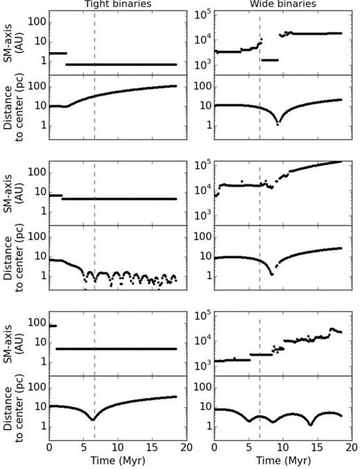
Evolution of individual binaries semimajor axis and distance to centre over time in the low-density 20 k particles models. The vertical dashed line marks the moment of deepest collapse t ≃ (t₁ + t₂)/2.

Open in new tab Download slide

6 DISCUSSION AND CONCLUSIONS

6.1 Discussion

In this paper, we have shown with numerical experiments that the dissolution of binary stars proceeds at a much higher rate in initially clumpy configurations. The two-body relaxation time of clumps of typical membership N_c = 50 is about six times shorter than the global free-fall time of the subvirial star-forming volume. As a result, binaries are destroyed at a rate ≈10 times higher in clumps than in the later stages of evolution, when clumps have merged and a cluster of stars achieves dynamical equilibrium. We have also highlighted that the transition between clumpy and equilibrium states is much sharper when N ≳ 10⁴: in such rich star-forming regions, the binary dissolution rate is well approximated with a linear relation in both the regimes. When N ≲ 10⁴, we find a more gradual transition (Fig. 5). These findings compare well with those from e.g. Parker et al. (2011) based on fractal models, where the mass segregation by collisional evolution was found also to be very significant early-on.

We presented in Section 4 an argument suggesting that the deeper gravitational potentials achieved through infall by larger N models should lead to the destruction of tighter binaries and hence a shift in the peak of the distribution of separations (see Figs 6 and 7). The net effect of increasing N from 1500 to 80 000, however, results mainly in a factor of ≈2 increase in the fraction of wide (a > 300 au) binaries being destroyed. Tighter binaries are largely unaffected. In particular, the peak in the initial distribution of separations at a ≃ 50 au is essentially unchanged. Consequently, the slope of the separation distribution for wide binaries steepens with N (i.e. the Gaussian shape is more skewed in richer models) in the early stages of the life of a cluster. This effect is offset slightly by the formation of new very wide binaries in the post-collapse evolution, when several stars move on radial, weakly bond orbits (see also Kouwenhoven et al. 2010; Moeckel & Clarke 2011). We have found the formation of wide a > 10⁴ au binaries to be statistically very similar regardless of the initial system density or membership, when set at the same evolutionary stage. One important difference is the higher speed achieved by outflowing wide binaries formed in denser systems. Runs with initial mean number density of 6 per pc³ developed outflows of velocities ≈2–3 km s⁻¹; denser runs with 400 per pc³ reached velocities twice as large. Proper motion studies may pick up this bulk motion. In terms of distance D, proper motion p, and timeline Δt_p, one finds a minimal velocity for detection v_p such that

\begin{equation} v_{\rm p} \gtrsim \frac{1}{2}\times 10^{-3} \frac{p}{1\mu ^{\prime \prime }} \frac{D}{100\, \mathrm{pc}} \frac{\text{yr}}{\Delta t_{\rm p}} \mathrm{km}\,\mathrm{s^{-1}} \. \end{equation}

(13)

The Gaia spacecraft's resolution reaches down to ≈26 μas at magnitude 15 (V band), with a five-year timeline and could detect such outflows out to a distance of ∼600 pc. Well-known star-forming regions such as the Orion Nebula or ρOphiucus are possible targets for such outflows. Brighter, young stars should allow a more precise determination of v_p and possibly set new constraints on the formation history of rich open clusters.

We also noted that very tight binaries (a ≲ 0.01 au) formed as a result of binary–binary exchange collisions, when a new binary is formed as a result of the collision between two existing ones. The process begins in the clumps at the start, and carries on throughout the duration of the runs. Statistically we found that ≈0.05 per cent of all binaries end up with a semimajor axis a < 0.6 au. While these are low-number statistics, these events are important because they involve the most massive stars of the models, and their rapid formation (on a time-scale of ∼1 Myr) has direct implication for the formation by merger of very massive stars/contact binaries. The shortest axis system that we found had a ≃ 0.01 au and a total mass of 18 M_⊙ (see Fig. 10). We observed similar trends in all the simulations, but noted that virtually no such tight binaries form in high-density runs. One important factor contributing to this situation is the increased collision velocities and (therefore) reduced effective interaction cross-sections in denser regions (the Safronov number Θ drops by a factor of ≈4). Another possibility comes from inspection of the time series of events from a subset of the runs, when we observe that the semimajor axis of very tight (a < 0.1 au) binaries continues to evolve right until the end of the simulations. This is a strong indication that these binaries are members of a compact hierarchical system. The very formation of the tight binaries may involve not just a pair of binaries, but a more complex situation involving a small number of stars (see e.g. Leigh & Geller 2013; Geller & Leigh 2015). We feel unable to disentangle the web of possible formation channels with confidence given the limited statistics of our sample of simulations. All calculations reported here where performed with a stellar IMF truncated at 30 M_⊙ and without stellar evolution. This brings up issues for the later stages of evolution when the system age exceeds 10 Myr. It will be important in future investigations of that formation scenario to include a full stretch of the stellar IMF and perform the time evolution of the stars simultaneously with the dynamics.

6.2 Conclusions

The main findings of this paper are as follows.

The HL fragmented systems host a population of ‘spontaneous’ wide binaries that form from phase-space correlations. The distribution of separations a of that population is bell-shaped with a peak shifting from a ≃ 2000 to 8000 au as the system mean density is decreased. The multiplicity fraction of that population increases with the mass of the primary, and matches the trend observed in the field for primaries of mass >2 M_⊙.
We presented a method allowing us to add to the spontaneous population a subpopulation of binaries in such a way that the final, total distribution of semimajor axis a and multiplicity fraction f_b matches targeted trends. We have implemented a version recovering the field distribution of Raghavan et al. (2010).
The clumps process binaries up to 10 times faster than a relaxed spherical configuration, while the deeper potential of large-N runs reached during the merging and relaxation phase means that about twice as many binaries are dissolved in rich open clusters as there are in small N ≲ 5000 systems.
Very tight and massive binaries, with semimajor axis a down to 0.01 au, and total mass up to 15 M_⊙, are formed first inside the clumps through exchange binary–binary interactions (cf. Fig. 10). Such tight binaries continue to form and evolve as the clumps merge and the star cluster relaxes to equilibrium. These binaries would form contact systems on a time-scale ∼1 Myr with an occurrence frequency of 0.2 binaries per 10 k stars per Myr.
Very wide binaries, of separation a up to 2.10⁵ au, are formed in the low-density volumes of ejected stars during the relaxation phase of the runs. The mean velocities of ≈2–6 km s⁻¹ of these stars mean that they are ideal targets for proper-motion studies by the Gaia programme.

Acknowledgments

We thank the anonymous referee for a constructive report which led to significant improvements of the paper. We also thank B. Goldman. M. Giersz, and E. Vesperini for discussions. We also gratefully acknowledge financial support from Institut National des Sciences de l'Univers through grant AO2011-684316.

1

Varying the number of neighbours in this range has no strong effect on the detection rate.

2

It should be noted that selection effects may at least in part explain such correlations; see e.g. De Rosa et al. (2014).

3

The original treatment by Spitzer fixed a thin (vertically mixed) disc crossed by a stellar cluster at high speed.

REFERENCES

Aarseth

S. J.

,

2003

,

Gravitational N-Body Simulations

.

Cambridge Univ. Press

,

Cambridge

, p.

430

Google Scholar

Google Preview

OpenURL Placeholder Text

WorldCat

Aarseth

S. J.

,

Lin

D. N. C.

,

Papaloizou

J. C. B.

,

1988

,

ApJ

,

324

,

288

Crossref

Search ADS

Allison

R. J.

,

Goodwin

S. P.

,

Parker

R. J.

,

de

Grijs R.

,

Portegies

Zwart S. F.

,

Kouwenhoven

M. B. N.

,

2009

,

ApJ

,

700

,

L99

Crossref

Search ADS

Anderson

J.

,

Piotto

G.

,

King

I. R.

,

Bedin

L. R.

,

Guhathakurta

P.

,

2009

,

ApJ

,

697

,

L58

Crossref

Search ADS

Bacon

D.

,

Sigurdsson

S.

,

Davies

M. B.

,

1996

,

MNRAS

,

281

,

830

Crossref

Search ADS

Basri

G.

,

Reiners

A.

,

2006

,

AJ

,

132

,

663

Crossref

Search ADS

Bate

M. R.

,

2012

,

MNRAS

,

419

,

3115

Crossref

Search ADS

Binney

J.

,

Tremaine

S.

,

2008

,

Galactic Dynamics

, 2nd edn.

Princeton Univ. Press

,

Princeton, NJ

Google Scholar

Google Preview

OpenURL Placeholder Text

WorldCat

Boily

C. M.

,

Athanassoula

E.

,

Kroupa

P.

,

2002

,

MNRAS

,

332

,

971

Crossref

Search ADS

Boily

C. M.

,

Nakasato

N.

,

Spurzem

R.

,

Tsuchiya

T.

,

2004

,

ApJ

,

614

,

26

Crossref

Search ADS

Caputo

D. P.

,

de

Vries N.

,

Portegies

Zwart S.

,

2014

,

MNRAS

,

445

,

674

Crossref

Search ADS

Casertano

S.

,

Hut

P.

,

1985

,

ApJ

,

298

,

80

Crossref

Search ADS

Chabrier

G.

,

2003

,

PASP

,

115

,

763

Crossref

Search ADS

Close

L. M.

,

Siegler

N.

,

Freed

M.

,

Biller

B.

,

2003

,

ApJ

,

587

,

407

Crossref

Search ADS

Da

Rio N.

,

Tan

J. C.

,

Jaehnig

K.

,

2014

,

ApJ

,

795

,

55

Crossref

Search ADS

Davies

B.

,

Figer

D. F.

,

Kudritzki

R.-P.

,

Trombley

C.

,

Kouveliotou

C.

,

Wachter

S.

,

2009

,

ApJ

,

707

,

844

Crossref

Search ADS

De

Rosa R. J.

et al. ,

2014

,

MNRAS

,

437

,

1216

Crossref

Search ADS

Dehnen

W.

,

1993

,

MNRAS

,

265

,

250

Crossref

Search ADS

Dorval

J.

,

Boily

C. M.

,

Moraux

E.

,

Maschberger

T.

,

Becker

C.

,

2016

,

MNRAS

,

459

,

1213

Crossref

Search ADS

Duchêne

G.

,

Kraus

A.

,

2013

,

ARA&A

,

51

,

269

Crossref

Search ADS

Duquennoy

A.

,

Mayor

M.

,

1991

,

A&A

,

248

,

485

Fischer

D. A.

,

Marcy

G. W.

,

1992

,

ApJ

,

396

,

178

Crossref

Search ADS

Foster

J. B.

et al. ,

2015

,

ApJ

,

799

,

136

Crossref

Search ADS

Fregeau

J. M.

,

Cheung

P.

,

Portegies

Zwart S. F.

,

Rasio

F. A.

,

2004

,

MNRAS

,

352

,

1

Crossref

Search ADS

Geller

A. M.

,

Leigh

N. W. C.

,

2015

,

ApJ

,

808

,

L25

Crossref

Search ADS

Goodwin

S. P.

,

Whitworth

A. P.

,

Ward-Thompson

D.

,

2004

,

A&A

,

423

,

169

Crossref

Search ADS

Goodwin

S. P.

,

Whitworth

A. P.

,

2004

,

A&A

,

413

,

929

Crossref

Search ADS

Heggie

D. C.

,

1975

,

MNRAS

,

173

,

729

Crossref

Search ADS

Heggie

D. C.

,

Mathieu

R. D.

,

1986

, in

Hut

P.

,

McMillan

S. L. W.

, eds,

Lecture Notes in Physics, Vol. 267, The Use of Supercomputers in Stellar Dynamics

.

Springer-Verlag

,

Berlin

, p.

233

Google Scholar

Google Preview

OpenURL Placeholder Text

WorldCat

Heggie

D. C.

,

Hut

P.

,

McMillan

S. L. W.

,

1996

,

ApJ

,

467

,

359

Crossref

Search ADS

Heggie

D. C.

,

Trenti

M.

,

Hut

P.

,

2006

,

MNRAS

,

368

,

677

Crossref

Search ADS

Hills

J. G.

,

1975

,

AJ

,

80

,

809

Crossref

Search ADS

Hubber

D. A.

,

Whitworth

A. P.

,

2005

,

A&A

,

437

,

113

Crossref

Search ADS

Hut

P.

,

1983

,

ApJ

,

268

,

342

Crossref

Search ADS

Hut

P.

,

Bahcall

J. N.

,

1983

,

ApJ

,

268

,

319

Crossref

Search ADS

King

R. R.

,

Parker

R. J.

,

Patience

J.

,

Goodwin

S. P.

,

2012

,

MNRAS

,

421

,

2025

Crossref

Search ADS

Korntreff

C.

,

Kaczmarek

T.

,

Pfalzner

S.

,

2012

,

A&A

,

543

,

A126

Crossref

Search ADS

Kouwenhoven

M. B. N.

,

Goodwin

S. P.

,

Parker

R. J.

,

Davies

M. B.

,

Malmberg

D.

,

Kroupa

P.

,

2010

,

MNRAS

,

404

,

1835

Kroupa

P.

,

1995a

,

MNRAS

,

277

,

1491

Crossref

Search ADS

Kroupa

P.

,

1995b

,

MNRAS

,

277

,

1507

Crossref

Search ADS

Kroupa

P.

,

1995c

,

MNRAS

,

277

,

1522

Crossref

Search ADS

Kroupa

P.

,

2001

,

MNRAS

,

322

,

231

Crossref

Search ADS

Kroupa

P.

,

2008

, in

Aarseth

S. J.

,

Tout

C. A.

,

Mardling

R. A.

, eds,

Lecture Notes in Physics, Vol. 760, The Cambridge N-Body Lectures

.

Springer-Verlag

,

Berlin

, p.

181

Google Scholar

Google Preview

OpenURL Placeholder Text

WorldCat

Kroupa

P.

,

Burkert

A.

,

2001

,

ApJ

,

555

,

945

Crossref

Search ADS

Larsen

S. S.

,

2004

,

A&A

,

416

,

537

Crossref

Search ADS

Leigh

N. W. C.

,

Geller

A. M.

,

2013

,

MNRAS

,

432

,

2474

Crossref

Search ADS

Lomax

O.

,

Whitworth

A. P.

,

Hubber

D. A.

,

Stamatellos

D.

,

Walch

S.

,

2015

,

MNRAS

,

447

,

1550

Crossref

Search ADS

Mac

Low M.-M.

,

Klessen

R. S.

,

2004

,

Rev. Mod. Phys.

,

76

,

125

Crossref

Search ADS

Marks

M.

,

Kroupa

P.

,

2012

,

A&A

,

543

,

A8

Crossref

Search ADS

Marks

M.

,

Kroupa

P.

,

Oh

S.

,

2011

,

MNRAS

,

417

,

1684

Crossref

Search ADS

Maschberger

T.

,

2013

,

MNRAS

,

429

,

1725

Crossref

Search ADS

Maschberger

T.

,

Clarke

C. J.

,

Bonnell

I. A.

,

Kroupa

P.

,

2010

,

MNRAS

,

404

,

1061

Crossref

Search ADS

Mason

B. D.

,

Gies

D. R.

,

Hartkopf

W. I.

,

Bagnuolo

W. G.

Jr,

ten

Brummelaar T.

,

McAlister

H. A.

,

1998

,

AJ

,

115

,

821

Crossref

Search ADS

Meylan

G.

,

Heggie

D. C.

,

1997

,

A&AR

,

8

,

1

Crossref

Search ADS

Mikkola

S.

,

1983

,

MNRAS

,

203

,

1107

Crossref

Search ADS

Mikkola

S.

,

1984a

,

MNRAS

,

207

,

115

Crossref

Search ADS

Mikkola

S.

,

1984b

,

MNRAS

,

208

,

75

Crossref

Search ADS

Moeckel

N.

,

Clarke

C. J.

,

2011

,

MNRAS

,

415

,

1179

Crossref

Search ADS

Nitadori

K.

,

Aarseth

S. J.

,

2012

,

MNRAS

,

424

,

545

Crossref

Search ADS

Parker

R. J.

,

Meyer

M. R.

,

2014

,

MNRAS

,

442

,

3722

Crossref

Search ADS

Parker

R. J.

,

Reggiani

M. M.

,

2013

,

MNRAS

,

432

,

2378

Crossref

Search ADS

Parker

R. J.

,

Goodwin

S. P.

,

Kroupa

P.

,

Kouwenhoven

M. B. N.

,

2009

,

MNRAS

,

397

,

1577

Crossref

Search ADS

Parker

R. J.

,

Goodwin

S. P.

,

Allison

R. J.

,

2011

,

MNRAS

,

418

,

2565

Crossref

Search ADS

Patience

J.

,

Ghez

A. M.

,

Reid

I. N.

,

Matthews

K.

,

2002

,

AJ

,

123

,

1570

Crossref

Search ADS

Portegies

Zwart S. F.

,

McMillan

S. L. W.

,

Gieles

M.

,

2010

,

ARA&A

,

48

,

431

Crossref

Search ADS

Preibisch

T.

,

Balega

Y.

,

Hofmann

K.-H.

,

Weigelt

G.

,

Zinnecker

H.

,

1999

,

New Astron.

,

4

,

531

Crossref

Search ADS

Press

W. H.

,

Teukolsky

S. A.

,

Vetterling

W. T.

,

Flannery

B. P.

,

2007

,

Numerical Recipes: The Art of Scientific Computing

, 3rd edn.

Cambridge Univ. Press

,

New York

Google Scholar

Google Preview

OpenURL Placeholder Text

WorldCat

Raghavan

D.

et al. ,

2010

,

ApJS

,

190

,

1

Crossref

Search ADS

Renaud

F.

,

Gieles

M.

,

Boily

C. M.

,

2011

,

MNRAS

,

418

,

759

Crossref

Search ADS

Roos

O.

,

2013

,

Master's thesis, Master thesis (unpublished)

Spitzer

L.

Jr

1958

,

ApJ

,

127

,

17

Crossref

Search ADS

Spitzer

L.

,

1987

,

Dynamical Evolution of Globular Clusters

.

Princeton Univ. Press

,

Princeton, NJ

Google Scholar

Google Preview

OpenURL Placeholder Text

WorldCat

Stahler

S. W.

,

2010

,

MNRAS

,

402

,

1758

Crossref

Search ADS

Tailo

M.

et al. ,

2015

,

Nature

,

523

,

318

Crossref

Search ADS

PubMed

Vesperini

E.

,

Chernoff

D. F.

,

1996

,

ApJ

,

458

,

178

Crossref

Search ADS

Ward-Duong

K.

et al. ,

2015

,

MNRAS

,

449

,

2618

Crossref

Search ADS

APPENDIX A: PHASE-SPACE CORRELATIONS

The global, isotropic expansion of a uniform self-gravitating body is found by integrating the equations of motion with an initial velocity field

\begin{equation} \boldsymbol {v} = \mathcal {H}\,\boldsymbol {x}, \end{equation}

(A1)

where |$\mathcal {H}$| is the HL parameter, a monotonically decreasing function of time. We want to show that the two-body correlation function defined around phase-space coordinates |${\rm d} \boldsymbol {x}^3 {\rm d} \boldsymbol {v}^3$| must peak when the HL expansion nears |$\mathcal {H} \rightarrow 0$|⁠. Let m₁ and m₂ be two stars of coordinates |$\boldsymbol {x}_1, \boldsymbol {x}_2$|⁠, respectively; their relative velocity follows from (A1) as

\begin{equation*} \boldsymbol {v}_{1,2} = \mathcal {H} (\boldsymbol {x}_1 - \boldsymbol {x}_2) \equiv \mathcal {H}\,\boldsymbol {l}. \end{equation*}

With the definition of the reduced mass μ = m₁m₂/M and total mass M = m₁ + m₂, the binding energy per mass of the stars reads

\begin{equation} E = - \frac{G \mu }{ || \boldsymbol {x}_1 - \boldsymbol {x}_2 || } + \frac{1}{2} \, \boldsymbol {v}_{1,2}^2 = - \frac{G\mu }{l} + \frac{1}{2} \mathcal {H}^2 l^2 \,. \end{equation}

(A2)

The binding energy E < 0 provided that |$l^3 < 2\,G \mu / \mathcal {H}^2$|⁠. If we use as characteristic separation the mean distance in the homogeneous sphere of radius R(t) (which encloses all the stars), then for a total of N stars one may write l ≈ R/N^1/3 and take |$m_1 = m_2 = \overline{m} = M / N$|⁠; then |$\mu = \overline{m}^2/N$| and the condition E < 0 becomes

\begin{equation*} R(t)^3 < \frac{2G\overline{m}}{\mathcal {H}^2}\,. \end{equation*}

In practice, R(t) reaches a maximum value in a finite time interval since the system as a whole is bound. Because |$\mathcal {H} \rightarrow 0$|⁠, there must be a time interval during which the inequality is (on average) everywhere satisfied. We anticipate most ‘spontaneous’ binary stars to form during that time interval.

The calculation presented above predicts that virtually all stars should end up in binaries of separation ≈l = R(τ)/N^1/3 (t = τ being the time when |$\mathcal {H} = 0$|⁠). This is not so in practice because the velocity field around t = τ is not the Hubble flow of equation (A1), but is approximately a Gaussian field due to the formation of clumps (cf. Dorval et al. 2016). Because of density enhancements, where the tidal field would be stronger, only a subfraction of stars eventually form wide binaries; we found about 10 per cent in a typical simulations.

This situation is different from the one addressed by Kouwenhoven et al. (2010) and Moeckel & Clarke (2011). These authors found very wide binaries to form in the tenuous haloes of dissolving supervirial star clusters. Kouwenhoven et al. (2010) found a formation rate of a few per cent for these wide binaries and a separation distribution peaking at about 10⁵ au. We also found a peaked distribution but with a peak value of about 10⁴ au or less (see Section 3.3). Inspection of HL fragmented configurations showed that the interclump distance is typically of the order of 10⁵ au or more, which may explain why binary stars of such wide separations do not form (they are disrupted by the tidal field of clumps).

We want to outline the basic procedure that would lead to the identification of all bound pairs (including multiple stars) for a general case. Let us work with the one-body phase-space distribution function |$f(\boldsymbol {x}, \boldsymbol {v}, t)$|⁠; the game, then, is to ride one of the stars (say, m_i) and seek out any other one that may lead to E < 0. To do so, one may define a Heaviside operator, |$H_e( \boldsymbol {x}- \boldsymbol {x}_i, \boldsymbol {v} - \boldsymbol {v}_i)$| such that H_e = 1 whenever E < 0 and H_e = 0 otherwise. For instance, if we set t = τ (no time integration or averaging) and sum over all pairs once only, we compute N_b pairs, so

\begin{equation*} N_b = \sum _{j=1}^N \sum _{i > j} H_e( \boldsymbol {x}_j- \boldsymbol {x}_i, \boldsymbol {v}_j - \boldsymbol {v}_i) f(\boldsymbol {x}_i, \boldsymbol {v}_i - \boldsymbol {v}_j, t). \end{equation*}

In integral form, this formalism would allow us to perform Monte Carlo draws from any functional form for the distribution function f. Binney & Tremaine (2008), section 7.5.8, give a numerical example for the case when |$f = \overline{\rho }(\boldsymbol {x},t) / \overline{m} \, \tilde{f}(\boldsymbol {v},t)$|⁠, with |$\overline{\rho }(\boldsymbol {x},t) / \overline{m} =$| constant and the velocity d.f. |$\tilde{f}(\boldsymbol {v},t)$| is a Maxwellian.

Download all slides

Month:	Total Views:
January 2017	4
February 2017	18
March 2017	9
April 2017	4
May 2017	5
June 2017	6
July 2017	1
August 2017	2
September 2017	2
October 2017	5
November 2017	2
January 2018	4
February 2018	7
March 2018	6
April 2018	1
May 2018	4
July 2018	3
August 2018	3
September 2018	2
November 2018	4
December 2018	3
February 2019	4
March 2019	5
May 2019	2
June 2019	2
July 2019	2
September 2019	2
October 2019	5
November 2019	1
December 2019	2
February 2020	6
March 2020	1
April 2020	5
May 2020	7
June 2020	7
July 2020	9
August 2020	7
September 2020	6
October 2020	4
November 2020	4
December 2020	1
January 2021	1
February 2021	3
March 2021	10
April 2021	6
June 2021	3
July 2021	5
August 2021	13
September 2021	2
October 2021	1
November 2021	8
December 2021	4
January 2022	1
February 2022	6
March 2022	6
April 2022	1
May 2022	3
June 2022	5
July 2022	11
August 2022	13
September 2022	17
October 2022	6
November 2022	5
December 2022	7
January 2023	4
February 2023	3
March 2023	3
April 2023	5
May 2023	5
June 2023	3
July 2023	4
August 2023	3
September 2023	2
October 2023	1
November 2023	8
December 2023	10
January 2024	4
February 2024	6
March 2024	2
April 2024	9
May 2024	3
June 2024	4
July 2024	16
August 2024	4
September 2024	6
October 2024	6
November 2024	6
December 2024	4
January 2025	6
February 2025	6
March 2025	11
April 2025	1
May 2025	3

Article Contents

Wide- and contact-binary formation in substructured young stellar clusters

Abstract

1 INTRODUCTION

2 INITIAL CONDITIONS FROM HUBBLE–LEMAîTRE FRAGMENTATION

2.1 Initial setup

2.2 Simulations

3 THE BINARY POPULATION

3.1 Detecting the binaries

3.2 Spontaneous binary fraction versus primary mass

3.3 Spontaneous semimajor axis distribution

3.4 Complete separation distribution: procedure

3.4.1 Binary parameter distributions

3.4.2 Results for N = 20 k models

4 EVOLUTION OF BINARY POPULATIONS

4.1 Results

4.2 Semimajor axis distributions

4.3 Tidal shocks

5 EXTREME TIGHT AND WIDE BINARIES

5.1 Tight binaries

5.2 Wide binaries

6 DISCUSSION AND CONCLUSIONS

6.1 Discussion

6.2 Conclusions

Acknowledgments

REFERENCES

APPENDIX A: PHASE-SPACE CORRELATIONS

Citations

Views

Altmetric

Email alerts

Astrophysics Data System

Citing articles via

Latest

Most Read

Most Cited

Article Contents

Wide- and contact-binary formation in substructured young stellar clusters Free

Abstract

1 INTRODUCTION

2 INITIAL CONDITIONS FROM HUBBLE–LEMAîTRE FRAGMENTATION

2.1 Initial setup

2.2 Simulations

3 THE BINARY POPULATION

3.1 Detecting the binaries

3.2 Spontaneous binary fraction versus primary mass

3.3 Spontaneous semimajor axis distribution

3.4 Complete separation distribution: procedure

3.4.1 Binary parameter distributions

3.4.2 Results for N = 20 k models

4 EVOLUTION OF BINARY POPULATIONS

4.1 Results

4.2 Semimajor axis distributions

4.3 Tidal shocks

5 EXTREME TIGHT AND WIDE BINARIES

5.1 Tight binaries

5.2 Wide binaries

6 DISCUSSION AND CONCLUSIONS

6.1 Discussion

6.2 Conclusions

Acknowledgments

REFERENCES

APPENDIX A: PHASE-SPACE CORRELATIONS

Citations

Views

Altmetric

Email alerts

Astrophysics Data System

Citing articles via

Latest

Most Read

Most Cited

This Feature Is Available To Subscribers Only

Wide- and contact-binary formation in substructured young stellar clusters