


Abstract
We study the resonant relaxation (RR) of an axisymmetric, low-mass (or Keplerian) stellar disc orbiting a more massive black hole (MBH). Our recent work on the general kinetic theory of RR is simplified in the standard manner by the neglect of ‘gravitational polarization’ and applied to a razor-thin axisymmetric disc. The wake of a stellar orbit is expressed in terms of the angular momenta exchanged with other orbits, and used to derive a kinetic equation for RR under the combined actions of self-gravity, 1 PN and 1.5 PN general relativistic effects of the MBH and an arbitrary external axisymmetric potential. This is a Fokker–Planck equation for the stellar distribution function (DF), wherein the diffusion coefficients are given self-consistently in terms of contributions from apsidal resonances between pairs of stellar orbits. The physical kinetics is studied for the two main cases of interest. (1) ‘Lossless’ discs in which the MBH is not a sink of stars, and disc mass, angular momentum and energy are conserved: we prove that general H-functions can increase or decrease during RR, but the Boltzmann entropy is (essentially) unique in being a non-decreasing function of time. Therefore, secular thermal equilibria are maximum entropy states, with DFs of the Boltzmann form; the two-ring correlation function at equilibrium is computed. (2) Discs that lose stars to the MBH through an ‘empty loss cone’: we derive expressions for the MBH feeding rates of mass, angular momentum and energy in terms of the diffusive fluxes at the loss-cone boundaries.
1 INTRODUCTION
Dense star clusters orbit massive black holes (MBHs) in galactic nuclei. Within the sphere of influence of the MBH, the inverse-square Newtonian gravity of the MBH is the dominant force on a star when its speed is non-relativistic. Were cluster self-gravity to be neglected completely, every star would orbit the MBH in a closed Keplerian ellipse. The orbits are not closed when the small perturbation due to self-gravity is taken into account; in addition to oscillations over the (fast) Kepler orbital time, the orbital elements of the ellipses also evolve over longer time-scales. This long-term behaviour is called secular evolution, for which there is a well-developed theory in planetary dynamics (Murray & Dermott 1999). In contrast to a planetary system, a low-mass star cluster orbiting an MBH is a many-body system, for which both the dynamics and the statistical mechanics are important. In Sridhar & Touma (2016a,b), hereafter referred to as Papers I and II, respectively, we presented a general theory of the secular evolution of these systems.
Let us consider a stellar system of size R with N ≫ 1 stars, each of mass m⋆, orbiting an MBH of mass M• . The typical Kepler orbital period, Tkep = 2π(R3/GM•)1/2, is the shortest time-scale in the problem. In common with other large N stellar systems, a Keplerian system may, in the first approximation, be treated in the ‘collisionless’ limit, N → ∞ and m⋆ → 0, while M = Nm⋆ is held constant. In this limit each star moves like a massless test particle that is acted upon by the MBH and the smooth mean gravitational field of the stellar system. For a low-mass stellar system, the total mass in stars, M = Nm⋆, is much smaller than M• ; the mass ratio, ε = M/M• ≪ 1, is an important small parameter. The Keplerian orbital elements of every stellar orbit evolve over secular times, Tsec = ε−1Tkep. In Paper I, we exploited the fact that there are two different time scales, Tkep and Tsec ≫ Tkep; thus, we began with the collisionless Boltzmann equation (CBE; Binney & Tremaine 2008), valid for a general stellar system, and averaged it over the fast Kepler orbital phase using the method of multiple time-scales. This resulted in a reduced description where each star is replaced by a Gaussian ring, which is a Keplerian ellipse whose eccentricity, inclination, apsidal angle and nodal longitude evolve over times Tsec, whereas the semi-major axis remains constant. The distribution function (DF) of Gaussian rings obeys a secular CBE, and hence many conclusions followed from general considerations: a secular Jeans theorem can be used to construct a rich variety of secular collisionless equilibria with greater ease than in the full, non-averaged dynamics; the linear instability of these equilibria is also simpler to study; and an arbitrary initial condition may be expected to undergo ‘violent’ (collisionless) relaxation to some coarse-grained secular equilibrium state, over times |${\sim }\, {\rm \text{a}\, few\,} T_{\rm sec}$|.
When N is large but finite, as is the case in practice, a collisionless equilibrium state is realized only in an approximate sense. The small graininess inherent in the sampling of such a state will make the stellar system evolve in time due to gravitational ‘collisions’ between the stars. Two-body encounters between stars enable exchanges of both energy and angular momentum with a coherence time of the order of the orbital time Tkep. The incoherent sum of many such encounters results in kinetic evolution over the two-body relaxation time Trelax = ε−2NTkep : some stars gain energy and increase their orbital radii while those that lose energy go into more tightly bound orbits, leading to a gravothermal catastrophe (Binney & Tremaine 2008). However Trelax is usually greater than the Hubble time for galactic nuclei of interest. Rauch & Tremaine (1996) proposed a more efficient process, called resonant relaxation (RR), which can be thought of as driven by gravitational interactions between pairs of Gaussian rings. Since the Keplerian energies (equivalently the semi-major axes) of Gaussian rings are conserved, they can only exchange angular momentum. This has a coherence time ∼ Tsec which is longer than the coherence time (Tkep) of two-body relaxation. The incoherent sum of many such encounters results in kinetic evolution over the RR time Tres = NTsec = εTrelax , which can be shorter than the Hubble time for galactic nuclei of interest.1 RR leads to a genuine equilibrium within a Hubble time (which can be expected to evolve very slowly due to two-body relaxation). In Paper II we presented a first-principles theory of RR, which is based on the rigorous kinetic theory of Gilbert (1968).
Gilbert's theory applies to general stellar systems and is based on a systematic 1/N expansion of the BBGKY hierarchy of equations:2 the O(1) secular theory describes collisionless mean-field dynamics, and the collisional theory emerges at O(1/N). In order to derive a theory for RR in Paper II, we orbit-averaged Gilbert's kinetic equations by using the method of multiple scales that was introduced in Paper I. A resonantly relaxing stellar system can be thought of as passing through a sequence of quasi-stationary, collisionless equilibria. The RR theory of Paper II places no restriction on either the spatial geometry or the orbital structure of the stellar system, so both of these could evolve with time. Scalar and vector RR are naturally treated on par as contributions arising from the apsidal and nodal resonances between stellar orbits. But this very generality of our theory of RR required a formulation in terms of the abstract, yet compact, Poisson-Bracket notation. The goal of the present work is to make concrete this abstraction and derive explicit formulae that describe the physical kinetics of an astrophysically interesting system.
The model stellar system must be as simple as possible, so we are able to see in explicit form how the kinetic theory works; the system must also be realistic enough to describe interesting physical phenomena such as the feeding of mass, energy and angular momentum to the MBH. Hence, we begin by considering stellar systems whose DFs possess high spatial symmetry. The simplest three-dimensional DFs are those corresponding to spherical, non-rotating systems. These could be reasonable approximations to the stellar nuclei of many galaxies, and it is important to work out their RR kinetics and the rates at which mass and stellar orbital energy are fed to the MBH. However, for the simplest case of a non-spinning (Schwarzschild) MBH, the inflow of stars cannot carry, by symmetry, a net angular momentum. This limitation can be overcome only by relaxing the requirement of complete spherical symmetry: one could introduce some net rotation in the DF or/and consider a spinning (Kerr) MBH. But an exactly spherical and rotating system is somewhat unnatural, and the exclusion of Schwarzschild MBHs seems rather extreme. Hence, it is useful to study RR in non-spherical and rotating DFs. This can be done – and it is important to do so – but it comes at the expense of working with a more complicated orbital structure. We need a simpler system in order to display the physical kinetics of RR as transparently as possible. Our choice is an axisymmetric Keplerian disc of stars confined to a plane, with the spin of the MBH (when it is non zero) directed perpendicular to the disc plane. We note that this limits our study to scalar RR.
Discs are naturally rotating and we may expect RR to feed angular momentum, in addition to mass and energy, to the MBH through a loss cone. Discs around compact objects are ubiquitous in the Universe; a two-dimensional system is, of course, an idealization of a realistic disc but it is often useful in the study of disc dynamics (Binney & Tremaine 2008). In particular, the exploration of the (secular) statistical mechanics of two-dimensional Keplerian discs by Touma & Tremaine (2014) brings important insights into the nature of secular thermal equilibrium, whereas a corresponding detailed study does not exist for three-dimensional systems. They consider both axisymmetric discs and non-axisymmetric discs. In this paper, we make a beginning by providing the kinetic theory of the approach to secular thermal equilibrium of razor-thin axisymmetric discs.
In Section 2, we recall the salient results of Papers I and II for a general Keplerian system orbiting an MBH. This generality is necessary because we introduce in Section 3 the ‘Passive Response Approximation’ (PRA) in the context of RR (the PRA is a standard simplification of the kinetic equations for plasmas and gravitating systems, wherein gravitational polarization is ignored). From Section 4 onward we specialize to the case of a razor-thin axisymmetric disc. The wake produced by a stellar orbit is expressed in terms of the angular momenta exchanged between two stellar orbits, now viewed as two gravitationally interacting Gaussian rings. In Section 5 we obtain an explicit form of the collision integral and use this to write the RR kinetic equation in the ‘conservation’ form. The kinetic equation is then cast in the Fokker–Planck form and the diffusion coefficients identified. The collision integral, the RR probability current density and the diffusion coefficients get contributions only from orbits that are in apsidal resonance. Formulae for the total mass, energy and angular momentum of the stellar disc are derived. In Section 6, we consider a ‘lossless’ stellar disc – a disc in which there is no loss of stars to the MBH. We demonstrate that the kinetic equation conserves total mass, angular momentum and energy, and prove an H-theorem on the non-decreasing nature of the time evolution of the Boltzmann entropy. Therefore, RR drives the system towards a stationary state of maximum entropy, which is a secular thermal equilibrium described by a DF of the Boltzmann form. The RR probability current density vanishes at equilibrium, but particle correlations do not. We calculate the two-ring correlation function at secular thermal equilibrium. In Section 7, we consider the disc with a loss cone and derive explicit formulae for the rates at which mass, angular momentum and energy are fed to the MBH. Conclusions follow in Section 8.
2 SECULAR THEORY OF KEPLERIAN STELLAR SYSTEMS
Here, we provide a brief review of some of the results of Papers I and II, which are needed later for elaborating the RR of axisymmetric discs. We consider a model system composed of N ≫ 1 stars, each of mass m⋆, orbiting an MBH of mass M• . The stellar system is Keplerian when the dominant gravitational force on the stars is the inverse-square Newtonian force of the MBH. An isolated and only mildly relativistic system is Keplerian when its total mass in stars, M = Nm⋆, is much smaller than M• ; then the mass ratio ε = M/M• ≪ 1 is a natural small parameter. The limiting case of negligible stellar self-gravity, ε → 0 , reduces to the Kepler problem of each star orbiting the MBH independently on a fixed Keplerian ellipse. An orbit is then conveniently described in six-dimensional phase space, in terms of the evolution of its Delaunay action-angle variables {I, L, Lz; w, g, h}. The three actions are |$I\,=\,\sqrt{GM_\bullet a\,}\,$|, |$L\,=\, I\sqrt{1-e^2\,}$| the magnitude of the angular momentum and Lz = L cos i the z-component of the angular momentum. The three angles conjugate to them are, respectively, w the orbital phase, g the angle to the periapse from the ascending node and h the longitude of the ascending node. The Kepler orbital energy Ek(I) = −1/2(GM/I)2 depends only on the action I. Hence, when ε = 0, all the Delaunay variables except w are constant in time; w itself advances at the (fast) rate 2π/Tkep = (GM•/a3)1/2.
When ε ≪ 1 and non-zero, the self-gravity is small but its effects build up over long times. Secular theory seeks to describe the average behaviour of quantities over (secular) times Tsec = ε−1Tkep , by averaging over the fast phase w. It should be noted that the stellar system must be stable on the fast time Tkep in order for the secular description to make sense (see footnote 4 of Paper I). Since w is no longer present in the secular theory, its conjugate action I is a conserved quantity; hence the semi-major axis of every stellar orbit is constant in time. Then, the stellar system can be described as a self-gravitating system of N Gaussian rings. Each ring is a point in five-dimensional ring space with coordinates |${\cal R}\equiv \lbrace I, L, L_z; g, h\rbrace$|, representing a Keplerian ellipse of given semi-major axis, eccentricity, inclination, periapse angle and nodal longitude. A ring can deform over secular times Tsec , under the combined action of mutual self-gravity between the rings, secular relativistic corrections and external gravitational fields (which can vary over times Tsec). This is represented by an orbit |${\cal R}(\tau )$|, with I = constant, parametrized by the slow time variable τ = ε(time).
2.1 Collisionless dynamics
2.2 Resonant relaxation
No-loss boundary conditions: when the MBH is not considered to be a sink of stars, the set of N rings is a closed system and the ring DF is normalized as |$\int F({\cal R}, \tau )\,{\rm d}{\cal R}=\ 1\,$|. Subject to this normalization |$F({\cal R}, \tau )$| can take any positive value at any location in |${\cal R}$|-space; in other words, the domain of F is all of |${\cal R}$|-space. Similarly, the domain of the wake function |$W({\cal R}\,\vert \,{\cal R}^{\prime }, \tau )$| is all of |${\cal R}$| and |${\cal R}^{\prime }$| spaces.
- Empty loss-cone boundary conditions: a star that comes close enough to the MBH will be either torn apart by its tidal field or swallowed whole by it. We can only require that at some initial time τ0,At later times τ > τ0, we will have |$\int F({\cal R}, \tau )\,{\rm d}{\cal R}\,\le \, 1\,$|. The loss of stars at small distances from the MBH can be simply modelled by an absorbing barrier: we assume that a star is lost to the MBH when its pericentre distance is smaller than some fixed value rlc, the ‘loss-cone radius’. When the loss cone is empty, stars belonging to the cluster must necessarily have pericentre radii a(1 − e) larger than rlc . Hence the domain of |$F({\cal R}, \tau )$| is restricted to regions of |${\cal R}$|-space in which I and L are large enough:(20)\begin{equation} \int F({\cal R}, \tau _0)\,{\rm d}{\cal R}\,=\, 1,\quad \mbox{initial normalization.} \end{equation}The boundary conditions on the ring DF and wake functions are(21)\begin{eqnarray} &&{I_{\rm lc} < I \quad \mbox{where}\quad I_{\rm lc} \,=\, \sqrt{GM_\bullet r_{\rm lc}}}\nonumber \\ &&{L_{\rm lc}(I) < L \,\le \, I, \quad \mbox{where}\quad L_{\rm lc}(I) \,=\, I_{\rm lc}\left[\,2 \,-\, \left(\frac{I_{\rm lc}}{I}\right)^2\,\right]^{1/2}.} \end{eqnarray}(22)\begin{eqnarray} F({\cal R}, \tau ) &=& 0\quad \mbox{for $I \le I_{\rm lc}\,$ and $\,L \le L_{\rm lc}(I)$,}\nonumber \\ W({\cal R}\,\vert \,{\cal R}^{\prime }, \tau ) \,&=& 0\quad \mbox{for $I, I^{\prime } \le I_{\rm lc}\,$ and $\,L \le L_{\rm lc}(I)$, $\,L^{\prime } \le L_{\rm lc}(I^{\prime })$.} \end{eqnarray}
Equation (15) for W and the kinetic equation for F – either equations (10)–(11) and (18) or (19a)–(19c) – together with suitable boundary conditions are the fundamental equations governing RR.
3 PASSIVE RESPONSE APPROXIMATION
We recall from equation (12), and the discussion following it, that the full RR kinetic theory applies to systems that evolve in a quasi-stationary manner through a sequence of secularly stable (collisionless) equilibria. This property is inherited by the above PRA integral expressions for wakes of various orders. Here F should be regarded as a slowly varying function of τ΄, with time-scale ∼ Tres ≫ Tsec ; this fact is used later in Section 4.2, to simplify in a standard manner the time integral for W(1).
The PRA has a history in both plasma physics and stellar dynamics. The Landau (1936) equations for electrostatic plasmas is a PRA of the equations of Balescu (1960) and Lenard (1960). The general collisional theory for stellar systems, which was initiated by Gilbert (1968), was simplified by Polyachenko & Shukhman (1982) through a PRA applied to systems with integrable mean-field Hamiltonians. They computed the integral for the irreducible part of the two-particle correlation function and showed that only the resonant part contributes to the kinetic evolution. They also proved an H-theorem and derived a Fokker–Planck equation for spherical stellar systems. There has been some work on the applications of the kinetic equation (in either the Gilbert form or the Polyachenko–Shukhman form) but we do not review this literature. Even in the more tractable PRA form, the Polyachenko–Shukhman kinetic equation applies to inhomogeneous systems, and computing interactions between realistic stellar orbits can be complicated. Further simplification can be achieved through a local approximation (Chandrasekhar) by assuming that stars encounter each other on constant velocity orbits. Then one descends from the Polyachenko–Shukhman equation to the familiar description of classical two-body relaxation given in Binney & Tremaine (2008).
The PRA wake is given in equation (26a) as a formal time integral over the histories of the two ring orbits |${\cal R}(\tau ^{\prime })$| and |${\cal R}^{\prime }(\tau ^{\prime })$| in the quasi-statically deforming secular equilibrium, |$F({\cal R}, \tau )$|. The formalism is general and does not require that the secular Hamiltonian, |$H({\cal R}, \tau )$|, be integrable (at fixed τ). However, matters simplify when the secular Hamiltonian is integrable (at fixed τ), because we can proceed with the calculation of the time integral using techniques similar to Polyachenko & Shukhman (1982). In the rest of this paper we apply the PRA equations to the RR of razor-thin axisymmetric discs.
4 WAKES IN A RAZOR-THIN AXISYMMETRIC DISC
A razor-thin (flat) disc corresponds to the idealized case when all N rings are confined to the xy plane. The angular momentum of every ring points along |$\pm \hat{z}$|, so a ring is specified by its semi-major axis, angular momentum and apsidal longitude. Ring space is three-dimensional: we write |${\cal R}= \lbrace I, L, g\rbrace$|, where L stands for the angular momentum which can now take both positive and negative values ( − I ≤ L ≤ I ), and g is the longitude of the periapse.7 Earlier formulae apply with |${\rm d}{\cal R}\equiv {\rm d}I\,{\rm d}L\,{\rm d}g$|. Ring space is topologically equivalent to |${R}^3$|, with I the radial coordinate, |$\arccos {(L/I)}$| the colatitude, and g the azimuthal angle.
4.1 Collisionless limit
All axisymmetric perturbations of F(I, L) give rise to nearby axisymmetric equilibria.
When (∂F/∂L) does not change sign anywhere in |${\cal R}$|-space, the DF is neutrally stable to modes of all m (where m is the azimuthal wavenumber).
Other stability results for F(I, L) are: non-rotating discs described by DFs that are even functions of L with empty loss cones (F/L non-singular when L → 0 ) are likely to be unstable to m = 1 modes (Tremaine 2005); Mono-energetic counter-rotating discs dominated by nearly radial orbits are prone to non-axisymmetric loss-cone instabilities of all m (Polyachenko, Polyachenko & Shukhman 2007).
4.2 Wake function
The physical meaning of these expressions is the following: ΔL/N is the net change in the specific angular momentum of ring |${\cal R}$|, due to the torques exerted on it by ring |${\cal R}^{\prime }$|. We recall from equation (13) that W/N is one of three components of the perturbation to the DF, resulting from the Rostoker–Gilbert gedanken experiment with rings. Then equation (44a) is just the standard PRA expression for the net change in the DF at any location |${\cal R}$|. The wake is proportional to the angular momentum exchanged between the rings.
The form of equations (44a) and (44b) for the wake, together with some of the symmetry properties of Ψ, allows us to draw some general conclusions. We recall from Paper I the ‘bare’ ring–ring interaction potential, Ψ, has the following symmetries:
P1: Ψ is a real function which is even in both L and L΄ .
P2: The apsidal longitudes g and g΄ occur in Ψ only in the combination |g − g΄|.
P3: Ψ is independent of both g and g΄ when one of the two rings is circular (i.e. when L = ±I or L΄ = ±I΄ or both).
P4: Ψ is invariant under the interchange of the two rings. This can be achieved by any of the transformations: {I, L}↔{I΄, L΄} , or g↔g΄ or both. In explicit form we have: Ψ(I, L, g, I΄, L΄, g΄) = Ψ(I΄, L΄, g, I, L, g΄), Ψ(I, L, g, I΄, L΄, g΄) = Ψ(I, L, g΄, I΄, L΄, g), which implies that Ψ(I, L, g, I΄, L΄, g΄) = Ψ(I΄, L΄, g΄, I, L, g).
We verify here that the wake satisfies some essential properties.
- The PRA wake function given by equations (44a) and (44b) must satisfy the two consistency conditions of equations (30). The first one states that there is no net mass in the wake of ring |${\cal R}^{\prime }$|. Since ΔL = ∂{ }/∂g, we have\begin{equation*} \int W({\cal R}, {\cal R}^{\prime }, \tau )\,{\rm d}{\cal R}\,=\, -\int {\rm d}I\,{\rm d}L \frac{\mathrm{\partial} F}{\mathrm{\partial} L}\int _0^{2\pi }{\rm d}g\,\Delta L \,=\, 0. \nonumber\end{equation*}The second identity requires that the net wake at any location |${\cal R}$|, due to all the rings, must vanish. Since ΔL = ∂{ }/∂g = −∂{ }/∂g΄ by property P2, we have\begin{equation*} \int W({\cal R}, {\cal R}^{\prime }, \tau )F({\cal R}^{\prime }, \tau )\,{\rm d}{\cal R}^{\prime } \,=\, -\frac{\mathrm{\partial} F}{\mathrm{\partial} L}\int {\rm d}I^{\prime }\,{\rm d}L^{\prime }\,F(I^{\prime }, L^{\prime }, \tau ) \int _0^{2\pi }{\rm d}g^{\prime }\,\Delta L \,=\, 0. \end{equation*}
When one of the two rings is circular, P3 implies that Ψ is independent of g and g΄. Hence ΔL = −ΔL΄ = 0 and |$W({\cal R}\,\vert \,{\cal R}^{\prime }, \tau ) = W({\cal R}^{\prime }\,\vert \,{\cal R}, \tau ) = 0$|. In other words, a circular ring neither produces a wake nor feels the wake of another ring.
5 KINETIC EQUATION FOR A RAZOR-THIN AXISYMMETRIC DISC
5.1 Collision integral
F1: the Cm are real functions that are even in L and L΄.
F2: the Cm are even in m: i.e. Cm = C−m .
F3: when either L = ±I or L΄ = ±I΄ or both, then Cm = 0 for all m ≠ 0.
F4: Cm(I, L, I΄, L΄) = Cm(I΄, L΄, I, L).
5.2 Kinetic equation
K1: K is a non-negative function.
K2: K(I, L, I΄, L΄) is an even function of L and L΄.
K3: when either L = ±I or L΄ = ±I΄ or both, then K = 0.
K4: K(I, L, I΄, L΄) = K(I΄, L΄, I, L) is invariant under the interchange (I, L) ↔ (I΄, L΄).
We now make an estimate of the RR time-scale implied by the Fokker–Planck equation (63). From equation (62c) we estimate that D ∼ K/NΩ , where we have used the fact that the DF is normalized as given in equation (54). From equation (56) for the kernel K in terms of the Fourier coefficients Cm, we have K ∼ Ψ2 . Using the definition of Ψ given in equation (3b), K ∼ (GM•/a)2 where a is a typical semi-major axis. The precession frequency Ω ∼ (GM•/a3)1/2 because time has been measured in terms of the slow time variable τ = εt. Then the diffusion coefficient D ∼ (GM•)3/2/Na1/2 . The RR time-scale, Tres , can be estimated by requiring that over times, δτ ∼ εTres, the typical value of 〈(δL)2〉 ∼ L2 ∼ GM•a . Then equation (65) gives Tres ∼ 〈(δL)2〉/εD ∼ (N/ε)(a3/GM•)1/2 ∼ N(Tkep/ε) = NTsec , as expected.
5.3 Mass, angular momentum and energy
We define the mass, angular momentum and energy of the stellar disc below. In Section 6 we will prove that these quantities are, as expected, conserved when there is no loss of stars to the MBH; hence the normalization of the DF f, given in equation (54), is valid for all τ. However, when stars are lost to the MBH this normalization is valid only at some initial time τ = τ0. At later times τ > τ0, we will have ∫ dI dL f(I, L, τ) < 1 , and the mass, angular momentum and energy of the stellar disc will be different; this fuelling of the black hole is treated in Section 7.
6 PHYSICAL KINETICS OF A RAZOR-THIN LOSSLESS DISC
Here, we study the general properties of a stellar disc when there is no loss of stars to the MBH. The domain of the DF f(I, L, τ) is the maximum allowed: −I ≤ L ≤ I and I ≥ 0 , shown as the shaded region in Fig. 1 lying between the boundaries L = ±I that mark the prograde and retrograde circular orbits. In the shaded region f can take any non-negative value, subject to the normalization of equation (54). Below we verify conservation of disc mass, angular momentum and energy. We also prove an H-theorem on the increase of the Boltzmann entropy and discuss secular thermal equilibrium.
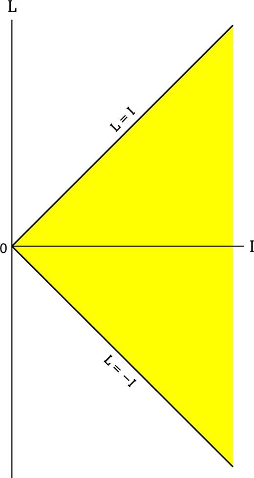
The region lying between the two diagonal lines (L = ±I) is the domain of the DF, f, when there is no loss of stars to the black hole. The upper and lower boundaries correspond to prograde and retrograde circular orbits, respectively; the current J vanishes on these boundaries.
6.1 Conserved quantities
6.2 H-theorem
6.3 Secular thermal equilibrium
The irreducible parts of the two-ring correlation function of equation (84) are proportional to β, and they vanish in the high temperature limit, which is consistent with the discussion following equation (48). Then the two-ring correlation function of equation (84) approaches its mean-field value, (4π2)−1feq(I, L)feq(I΄, L΄).
By a stability criterion proved in Paper I (mentioned in Section 4.1) these very hot DFs are dynamically stable to all axisymmetric and non-axisymmetric secular perturbations, because (∂feq/∂L) has the same sign as the constant γ, for all I and L.
Thermal stability of feq to axisymmetric perturbations can be studied by linearizing the kinetic equation (57) about feq. The thermal stability problem for non-axisymmetric perturbations is an important problem that needs to be formulated by going back to the PRA kinetic equation (28).
7 BLACK HOLE FUELLING RATES
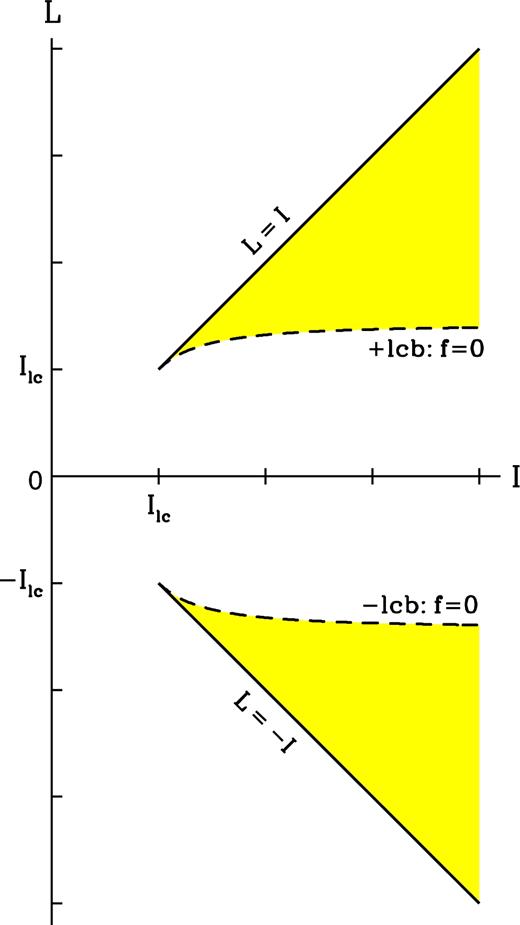
The domain of the DF, f, when stars are lost to the black hole through an empty loss cone. The domain is the union of the two disjoint wedge-like regions that are symmetric about the I-axis. The tip of the upper wedge is at I = L = Ilc and the tip of the lower wedge is at I = −L = Ilc. The DF vanishes on the dashed lines corresponding to prograde (+) and retrograde (−) loss-cone boundaries (‘lcb’).
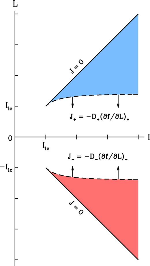
The probability current density J(I, L, τ) at the boundaries. J = 0 on the upper and lower boundaries marking the prograde and retrograde circular orbits. J = J+(I, τ) ≤ 0 on the +lcb, and J = J−(I, τ) ≥ 0 on the −lcb.
Equations (96), (98) and (101) give the rates at which RR feeds mass, angular momentum and energy to the MBH in simple and readily interpretable forms in terms of the currents of stars that pass through the loss-cone boundaries in (I, L) space. The boundary currents are diffusive in nature and given by equations (92a) and (92b), with the diffusion coefficients determined self-consistently by the DF as given in equations (93a) and (93b).
8 CONCLUSIONS
Our goal in Papers I through III is to formulate a theoretical framework describing the secular dynamics and statistical mechanics of a low-mass (or ‘Keplerian’) stellar system orbiting a MBH. In Papers I and II we derived the equations governing the collisionless and collisional (‘RR’) evolution, respectively, of general Keplerian systems. Here, in Paper III, we have simplified the RR kinetic equation and applied it to understand the physical kinetics of razor-thin axisymmetric Keplerian stellar discs.
RR evolution is driven by |$F^{(2)}_{\rm irr}({\cal R}, {\cal R}^{\prime }, \tau )$|, the ‘irreducible part of the two-ring correlator’, which measures the ring–ring correlations that develop over time, due to mutual stochastic torquing. This is conveniently calculated in terms of a related quantity, |$W({\cal R}\,\vert \,{\cal R}^{\prime }, \tau )$|, the ‘wake of |${\cal R}^{\prime }$| at |${\cal R}$|’, which has a nice physical interpretation as the linear collisionless response of the stellar system to the act of removing any one ring and re-introducing it into any specified ring orbit which arrives at |${\cal R}^{\prime }$| at time τ . Even though the equation governing W is simpler than the one governing |$F^{(2)}_{\rm irr}$|, it is still a linear, partial integro-differential equation in six variables. Our first result in this paper is the introduction of the ‘PRA’, which is an iterative scheme by which successive approximations to the wake can be generated. The lowest-order PRA ignores the effects of the gravitational polarization of the wake on its own evolution. The wake is then expressed as a time integral over the mutual interactions between two rings, over their entire past orbital histories (equation 26a). This can be used to derive the PRA kinetic equation (i.e. 29a–29c), which applies to a general Keplerian system; this equation can be thought of as the secular analogue of equations (1)–(3) of Polyachenko & Shukhman (1982).
We then applied the PRA to razor-thin axisymmetric discs described by DFs of the form F(I, L, τ). Equations (44a) and (44b) show that the PRA wake takes a simple form: with |${\cal R}= (I, L, g)$| and |${\cal R}^{\prime } = (I^{\prime }, L^{\prime }, g^{\prime })$|, we have |$W({\cal R}\,\vert \,{\cal R}^{\prime }, \tau ) = - (\mathrm{\partial} F/\mathrm{\partial} L)\,\Delta L$|, where |$\Delta L({\cal R}, {\cal R}^{\prime })$| is the angular momentum change experienced by a ring at |${\cal R}$| due to the torque exerted on it by the ring at |${\cal R}^{\prime }$| during the entire past history of their interaction. This form has a simple physical interpretation: W is the perturbation to F, accounting for the gain and loss of rings in an elemental volume around |${\cal R}$|, due to torquing by |${\cal R}^{\prime }$|. The wake can be decomposed into a ‘resonant’ and a ‘non-resonant’ part (equations 50a–50c), where the resonance referred to is between the apsidal precession rates of pairs of stellar orbits. Only the resonant part of the wake contributes to the collision integral, and determines RR evolution. This is physically reasonable, because we expect the accumulated mutual torque between two rings to average to zero when they are not resonant.
We then derive the PRA kinetic equation governing the RR evolution of F. This is given in equations (57) and (58) in the ‘conservation’ form’, where the probability density current of the RR flow in (I, L) space is seen to get contributions only from the resonant orbits. Since the I of every ring is constant, the current density is directed only along the L direction. The PRA kinetic equation can also be put in a self-consistent Fokker–Planck form, equation (63), with the diffusion coefficients determined self-consistently by the DF, as given by equations (64), (62b) and (62c).11 The nice thing about the Fokker–Planck form is the ready interpretation of the diffusion coefficients in terms of the average characteristics, per unit time, of the random changes in the specific angular momentum of a ring (see equation 65).
The broad features of the physical kinetics of RR were studied for the two major cases of interest, corresponding to the two different boundary conditions under which the kinetic equation is to be solved. These are (a) ‘Lossless’ discs in which the MBH is not a sink of stars (Section 6), and (b) discs which feed stars to the MBH through an ‘empty loss cone’ (Section 7). We obtained the following results.
Since the MBH does not consume stars, total disc mass, angular momentum and energy are all conserved. A general H-function can either increase or decrease during RR, but the Boltzmann entropy is (essentially) unique in being a non-decreasing function of time. It follows that maximum entropy states are also states of secular thermal equilibrium, and their DFs have the Boltzmann form, investigated by Touma & Tremaine (2014) for the limit in which all rings share the same semi-major axis. As a bonus we get a formula for the two-ring correlation function at equilibrium.
A star that comes close enough to the MBH will be either torn apart by its tidal field or swallowed whole by it. The stochastic evolution of the orbital angular momenta during RR evolution can make a star lose enough angular momentum for its pericentre to come closer than some minimum distance from the MBH; then the star is counted as lost to the MBH within a Kepler orbital period (which is essentially instantaneous when compared with secular or RR time-scales). This is modelled by an ‘Empty loss-cone’ boundary condition in (I, L) space, through which stars are lost to the MBH (see Figs 2 and 3). Equations (96), (98) and (101) give the rates at which RR feeds mass, angular momentum and energy to the MBH. These are given in terms of the currents of stars that pass through the loss-cone boundaries. The boundary currents are diffusive in nature and given by equations (92a) and (92b), with the diffusion coefficients determined self-consistently by the DF and given in equations (93a) and (93b).
All of these properties are valid for axisymmetric discs, allowing for 1 PN and 1.5 PN general relativistic effects on apsidal precession, as well as the gravity of an arbitrary axisymmetric external potential.
Having established an overall picture of the physical kinetics, it is necessary to compute and understand how RR affects orbits of different semi-major axes and eccentricities. Below are three interesting ways in which the present work can be taken forward:
Touma & Tremaine (2014) solved for maximum entropy equilibria of self-gravitating Keplerian discs, in the case when all stars have the same semi-major axis. Both axisymmetric and non-axisymmetric secular thermal equilibria were included. They found that a significant fraction of the axisymmetric equilibria were not really states of maximum entropy but saddle points, and are thermodynamically12 unstable to bifurcations favouring lopsided discs at the same energy and angular momentum. The symmetry breaking equilibria were solved for numerically and found to be generically rotating. The axisymmetric equilibria which were thermodynamically unstable were also found to be dynamically unstable, in the sense of the linearized ring CBE (whereas thermodynamic stability implies dynamical stability, thermodynamic instability does not imply dynamical instability). When followed into the non-linear regimes through numerical simulations, the dynamical instabilities saturated and relaxed into lopsided, uniformly precessing configurations. To be able to describe complex processes such as these requires (i) using the methods of Paper I to first construct generic lopsided and rotating collisionless equilibria which are also dynamically stable, and (ii) generalizing the approach of the present work to derive a kinetic equation for the RR of these broken-symmetry equilibria.
The RR kinetic theory of Paper II applies to general stellar distributions, and needs to be developed for fully three-dimensional systems. The simplest are spherical systems around a non-spinning MBH, whose orbital structure is as simple as the axisymmetric discs we studied in this paper. The difference now is that we need to consider the gravitational interactions between pairs of mutually inclined stellar orbits. This adds to the technical complexity of Fourier expansions, but the physical kinetics of RR can be expected to be as simple as it is for two-dimensional axisymmetric discs: we expect to find a kinetic equation of the Fokker–Planck form, with an H-theorem and secular thermal equilibrium of the Boltzmann form for a lossless system, and diffusive loss-cone feeding of mass and energy to the MBH.
Three-dimensional axisymmetric systems are naturally rotating, and we expect RR to feed the MBH with mass, energy and angular momentum. It is also fortuitous that the secular dynamics of these systems is completely integrable with I, Lz and H(I, L, Lz, g) being three isolating integrals (Sridhar & Touma 1999; Sambhus & Sridhar 2000).
Acknowledgments
We are grateful to Jerome Perez, Stephane Colombi and the Institut Henri Poincaré for hosting us when a part of this work was done. We thank Scott Tremaine for comments on an earlier draft.
The typical angular momentum (per unit mass) of a test ring is |$L\sim \sqrt{GM_\bullet a}$| where a is its semi-major axis. The torque experienced by the test ring, due to all the other rings, is |${\cal N}\sim (Gm_\star /a)N^{1/2}$|. Acting over a coherence time Tsec, this causes a change in L of the order of |${\cal N} T_{\rm sec}$|. Over longer times t ≫ Tsec the net change in L is |${\sim\, }{\cal N} T_{\rm sec}(t/ T_{\rm sec})^{1/2}$|, which is of the order of L when t ∼ NTsec = Tres.
The BBGKY hierarchy applies to many-body systems and has been used to derive the well-known Boltzmann equation for dilute gases and the Balescu–Lenard equation for electrostatic plasmas (Liboff 2003). One begins with the N-particle DF obeying the Liouville equation in 6N-dimensional phase space and integrates this over various phase space coordinates. This gives a hierarchy of equations for ‘reduced’ DFs, where the equation for the s-particle DF (with 1 ≤ s ≤ N − 1) depends on the (s + 1)-particle DF. The aim is to derive a closed equation for the one-particle DF in six-dimensional phase space by closing the hierarchy of equations by exploiting a small parameter.
Here, |$\Psi ({\cal R}, {\cal R}^{\prime })$| is proportional to the gravitational interaction potential energy between two rings, |${\cal R}$| and |${\cal R}^{\prime }$|, and has been scaled in a manner such that the equations of motion contain only quantities of order unity.
The typical time-scale of growth of a secular instability is Tsec, which is much shorter than the RR time-scale Tres = NTsec. Hence, the collisional terms, as discussed in Section 2.2, may be neglected while considering the dynamical stability of a secular equilibrium.
In the course of RR evolution, it may happen that a system goes through a sequence of stable secular equilibria and arrives at one which is secularly unstable. Then RR evolution would have tipped the system into an instability which will grow and saturate (due to collisionless relaxation) on the short time-scale Tsec; clearly the collision terms can be ignored while describing this fast process. The new equilibrium state is evidently stable, and subsequent RR evolution is described as given above.
The decomposition of the collision integral into dissipative and fluctuating components is traditional, and follows from the theory for a general stellar system. In Gilbert's words (see section V of Gilbert 1968), ‘The first of these clearly represents the deceleration of a star by its associated polarization cloud. The second term represents the effect on a star of the rapidly fluctuating, random fields produced by its neighbors.’ We are dealing with the secular version which is valid for Keplerian stellar systems.
This is the convention for the symbols (L, g) we use in the rest of this paper.
Hence the theory does not apply to very cold discs violating the Toomre (1964) criterion, because they are unstable to axisymmetric modes growing over times ∼ Tkep. So the discs we study are understood to have velocity dispersions large enough to make them stable to fast modes.
As earlier the normalization of equation (54) is true for all τ only in the conservative case of no loss of stars to the MBH. When the MBH is a sink of stars, the above normalization holds only at some initial reference time τ = τ0 when the disc mass is M.
These are related to the original Lagrange multipliers by ln A = ( − 1 + B − β΄MEk), β = β΄Mε and γ = γ΄M .
This is a special case of a more general result derived in Polyachenko & Shukhman (1982): the lowest-order PRA kinetic equation for a general stellar system with integrable mean-field Hamiltonian can be expressed in a self-consistent Fokker–Planck form.
Here, ‘thermodynamically’ refers to the thermodynamics of a large number of Gaussian rings. Since the semi-major axis of every ring is a fixed constant, the phase space is finite and the problem is well-defined, unlike the case of a general self-gravitating system.
