


Abstract
We study AGN emission line profiles combining an improved version of the accretion disc-wind model of Murray & Chiang with the magnetohydrodynamic (MHD) model of Emmering et al. Here, we extend our previous work to consider central objects with different masses and/or luminosities. We have compared the dispersions in our model C iv line-width distributions to observational upper limit on that dispersion, considering both smooth and clumpy torus models. Following Fine et al., we transform that scatter in the profile line-widths into a constraint on the torus geometry and show how the half-opening angle of the obscuring structure depends on the mass of the central object and the accretion rate. We find that the results depend only mildly on the dimensionless angular momentum, one of the two integrals of motion that characterize the dynamics of the self-similar ideal MHD outflows.
1 INTRODUCTION
Broad emission lines (BELs) are a spectral signature of type 1 active galactic nuclei (AGNs). Lines due to high-ionized species are generally single-peaked and blueshifted with respect to the systemic velocity (e.g. Sulentic et al. 1995; Sulentic, Marziani & Dultzin-Hacyan 2000; Vanden Berk et al. 2001). Although photoionization is well determined as the primary physical mechanism for their production, a detailed description of the region where the BELs originate is still an open question (e.g. Sluse et al. 2011; Chelouche & Zucker 2013; Grier et al. 2013). As the BLR is spatially unresolved, its structure and dynamics remain unclear and it is only through indirect methods that it can be studied.
Reverberation mapping (RM) is one of the few available such methods. It relies on the time lag in response to the BLR to variability of the continuum (see e.g. the review by Peterson 2006). In particular, RM studies in several AGNs have shown that the BLR is a stratified structure (e.g. Peterson & Wandel 2000): within the same AGN, the high-ionization lines are produced closer to the central source than the low-ionization lines.
Among the different competing and/or complementary models that have been developed to explain the nature of the BLR are discrete clouds and disc winds (see brief reviews by e.g. Eracleous 2006; Everett 2007). Broad-line cloud models describe this region as composed of numerous optically thick clouds that, photoionized by the continuum-source emission, are the emitting entities responsible for the observed lines. This model successfully explains many of the observed spectral features, but also leaves several unsolved issues, such as the formation and confinement of the clouds.
In models of outflowing gas, two major accelerating mechanisms have been invoked: magnetohydrodynamic (MHD) driving (e.g. Blandford & Payne 1982; Emmering, Blandford & Shlosman 1992; Contopoulos & Lovelace 1994; Kazanas et al. 2012), and radiative acceleration (e.g. Murray et al. 1995; Kurosawa & Proga 2009). In some of these wind models, the flow is assumed to be continuous (e.g. Königl & Kartje 1994; Murray & Chiang 1997), while in others, it contains embedded inhomogeneities or clouds (e.g. Bottorff et al. 1997). Both of these types of models have had some success in fitting AGN observations. The spectral line shapes can be used as a tool to study the kinematics and physics of plasmas in AGNs. One additional important motivation of wind BLR models is that they provide a feasible feedback mechanism to the host galaxy, thus regulating the co-evolution suggested by the solid relationships observationally found between the mass of the central object and some of the galaxy properties (e.g. Marconi & Hunt 2003; Häring & Rix 2004; Gültekin et al. 2009). It is also worth mentioning that the wind scenario offers the explanation least conflicting with the existence of a small group of AGN that show double-peaked line profiles (generally, Balmer lines) in their spectra and with the fact that some among them fluctuate between a double- and a single-peaked profile (e.g. Eracleous & Halpern 2003; Flohic, Eracleous & Bogdanović 2012). In addition, the model high-velocity component of the wind naturally explains the existence of blueshifted broad absorption lines (BALs) seen in an optically selected subset of the quasar population, known as BAL quasars (Murray et al. 1995; Elvis 2000).
Because BELs are produced close to the central engine, they carry important information on that region of the phenomenon (Sulentic et al. 2000). Hence, accurate emission line models are important for studying AGN properties, such as black hole masses and accretion rates and put constraints on the unification paradigm. Indeed, due to their ubiquity, some authors (e.g. Richards 2012) regard emission lines as a more powerful tool to studying AGN than absorption lines, because the latter are only present in a fraction of the quasar population.
We study AGN emission line profiles combining an improved version of the accretion disc-wind model of Murray & Chiang (1997) with the MHD driving of Emmering et al. (1992). Here, we present the extension of our previous work in Chajet & Hall (2013, Paper I hereafter), considering a range of masses and luminosities. We have compared the averages in our model C iv line-width distributions to the observational results of Fine et al. (2010), considering a smooth torus model. Additionally, we performed a similar study considering a clumpy torus (Nenkova et al. 2008).
The plan of the paper is as follows. In Section 2, we review our modifications to the Murray & Chiang (1997) disc-wind model. In Section 2.1, we outline the basics of MHD winds, with emphasis on the description of Emmering et al. (1992) and show how we constructed our combined model. Section 3 presents the C iv line profiles obtained with this model, and discusses their characteristics. In Section 4, using observational constraints on the dispersion of the line-widths, we derive constraints on the putative torus applicable to the various combinations of mass and Eddington ratio that we have considered. We explore both homogeneous (Section 4.2) and clumpy torus (Section 4.3) prescriptions as the obscuring structure. In Section 5, we discuss how different values of the dimensionless angular momentum parameter λ affect the results. We have considered two different values of λ and run simulations using λ = 10 and λ = 30. These values were chosen to match those used by Blandford & Payne (1982) and Emmering et al. (1992), respectively. In Section 6, we discuss our results and outline some possible ways for future exploration or improvement, and in Section 7, we present our conclusions.
2 MODEL DESCRIPTION
In Paper I, we presented our hybrid model, that combines the disc-wind model of Murray & Chiang (1997, hereafter MC97) with the MHD driving of Emmering et al. (1992) and here we include a brief description of it, that is applied to generate emission lines from AGNs.
We assume an azimuthally symmetric, time-independent disc and wind. The lines arise at the base zem of an emission region of thickness lem ≪ zem, at an angle β of the disc plane. This angle can, in principle, be a function of the radius, but we have adopted a fixed value. The wind streamlines make an angle of ϑ(r, z) relative to the disc plane.
Fig. 1 depicts the system geometry and shows streamlines for two different launch angles.
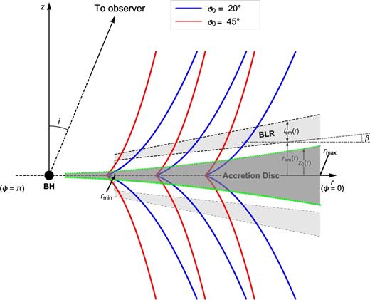
Streamlines for two different launch angles: |$\vartheta _0=20^\circ , 45^\circ$|. The disc midplane is assumed to lie in the z = 0 plane and the disc is assumed to be opaque, such that the observer, at an angle i from the +z axis, sees only the upper quadrants. The lower dashed line represents the base of the emitting region, tilted by an angle β with respect to the disc plane. The BLR is a layer of thickness lem(r) beginning a distance zem(r) above the disc mid-plane and spanning radii rmin < r < rmax. The height of the disc continuum photosphere is z0(r), where r is the cylindrical radial coordinate. The disc wind lies at z(r) > zem(r), and the emitting region for a given line is near the base of the wind, at zem(r) < z < zem(r) + lem(r) above the disc mid-plane.
The dependences of the quantities qtt(r, ϕ, i) and Q(r, ϕ, i) on the different parameters are rather complex to make a clear comparison in the general case. We will, then, discuss this point in Section 3.
2.1 Ideal MHD wind launching
Magnetic acceleration of outflows has been often suggested in the literature as an efficient means of removing excess of angular momentum from the accreting material (e.g. Blandford & Payne 1982; Contopoulos & Lovelace 1994; Königl & Kartje 1994; Everett 2005). The standard non-relativistic ideal MHD wind equations are presented in (e.g.) the above mentioned references, as well as in Paper I. In steady state (i.e. ∂/∂t = 0) and assuming axisymmetry (i.e. ∂/∂ϕ = 0), the solutions have a number of conserved quantities along each magnetic field line (e.g. Mestel 1968), that impose constraints to the flow dynamics. These are the mass to magnetic flux ratio, |$\frac{k}{4 \pi } = \frac{\rho \, V_{\rm p}}{B_{\rm p}}$|; specific angular momentum, |$l = r \left(V_{\rm \phi } - \frac{B_\phi }{k} \right)$| and specific energy, |$e =\frac{{V}^2}{2} + h + \Phi _{\rm g} - \frac{ r \Omega B_{\phi } }{k}$|, where the subscripts p and ϕ correspond respectively to the poloidal and azimuthal components of the velocity, V, and magnetic, |${\boldsymbol {B}}$|, vector fields; ρ is the gas density; Φg, the gravitational potential; and h and Ω are the specific enthalpy and the angular velocity, respectively.
An important quantity defined for magnetized fluids is the so-called Alfvén Mach number. The square of this quantity is defined as |$m =V_{\rm p}^2/V_{\rm Ap}^2$|, where VAp is the poloidal component of the Alfvén velocity |${V}_{\rm A} = \frac{{\boldsymbol {B}}}{\sqrt{4 \pi \, \rho }}$| which is the characteristic velocity of the propagation of magnetic signals in an MHD fluid. The Alfvén radius rA is the point on each poloidal field line where m = 1; the loci of all rA define the Alfvén surface. The subscript ‘A’ refers, hereafter, to quantities evaluated at the Alfvén point.
2.1.1 Blandford and Payne MHD wind solution
The self-similar scaling of the magnetic field amplitude B, and gas density ρ with the spherical radial coordinate r is given, in the general case (e.g. Emmering et al. 1992; Contopoulos & Lovelace 1994; Kazanas et al. 2012), by |$\rho \propto r_0^{-b}$|, for which |$B \propto r_0^{-(b+1)/2}$|. The BP82 solution is a particular case corresponding to b = 3/2. The magnetic field and density at arbitrary positions can be then written, in accordance with the self-similarity Ansatz (equation 7), as |${{\boldsymbol {B}} }= B_0(r_0) {{\boldsymbol {b}}}(\chi )$| and ρ = ρ0(r0)ϱ(χ). On the disc plane, the rotational velocity, Vϕ, is Keplerian and scales as |$V_{\phi } \propto r_0^{-1/2}$|. The functions ξ(χ), f(χ) and g(χ) have to satisfy the flow MHD equations subject to the above scalings of ρ, B, and Vϕ and boundary conditions. In particular, at the disc surface ξ(0) = 1, f(0) = 0 and g(0) = 1.
The parameters of the model are the dimensionless expressions of the integrals of motion: ε = e/(GM/r0), λ = l/(GMr0)1/2 and |$\kappa = k(1+\xi ^{\prime 2}_0) \left[(GM/r_0)^{1/2}/B_{0}\right]$|. An extra parameter is the value of the derivative |$\xi ^{\prime }_0$| of the self-similar function ξ at the disc surface. However, due to the regularity conditions that must be satisfied, these parameters are not independent. In particular, the value of |$\xi ^{\prime }_0\equiv \xi ^{\prime }(\chi =0)$| must be chosen to ensure the regularity of the solution at the Alfvén point. That reduces the degrees of freedom of the solutions, which are then parametrized by two numbers.
BP82 studied outflows that become super-Alfvénic (i.e. m > 1) at a finite height above the disc. The asymptotic conditions for such flows admit two kind of solutions that depend on the location of the fast-mode Mach number n above the disc.
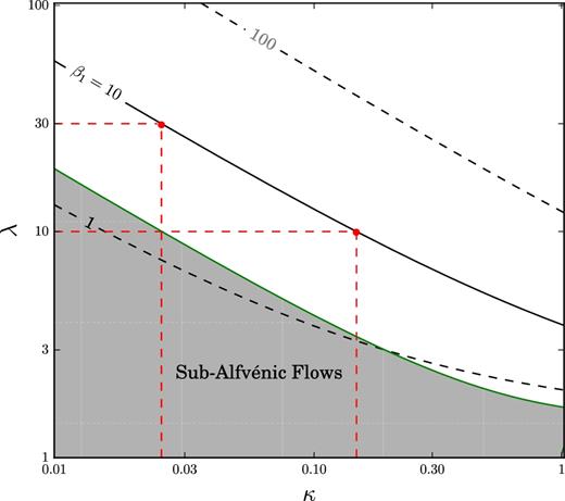
Contour plot analogous to fig. 2 of BP82. Each contour corresponds to a value of the quantity β1, defined in equation (9), which is fixed for a given problem. The solid contour corresponds to β1 = 10 and the possible (κ, λ) pairs for our problem, set by the condition in equation (12) imposed by the Emmering et al. (1992) choice of parameters. The dashed red lines locate the two points (also marked in red) for which we have explored in this work. Flows in the grey-shadowed region satisfy the condition κλmin(2λmin − 3)1/2 < 1, and will never become super-Alfvénic (|$4 \pi \rho \,V_{\rm p}^2 > B_{\rm p}^2$|).
2.1.2 Emmering et al. (1992) model
The EBS92 work was intended to support the cloud scenario of the BLR, and thus the authors proposed that the emission lines arise in clouds confined by an MHD flow. However, we follow MC97 and MC98 in assuming that the lines form in a continuous medium. We consider line emissivity obtained by a cloudy photoionization model, different from either of the emissivity laws adopted by EBS92. Two of those emissivity models include electron scattering, which is not considered in our model. In EBS92, both the dimensionless angular momentum λ and the launch angle are fixed. We, on the other hand, varied those parameters to study their effect on the profiles. Note also that while EBS92 obtains the line luminosity integrating in the two poloidal variables, we include the z-integral in the optical depth expression, already incorporated in equation (2).
3 LINE PROFILES
In Paper I, we applied the modified model described above to our fiducial case, characterized by mass M = 108M⊙ and luminosity L1350 (defined below) 1046erg s−1, and considered a dimensionless specific angular momentum λ = 10. We then studied several combinations of inclination angles, in the range |$5^\circ \leqslant i \leqslant 84^\circ$| and launch angles |$6^\circ \leqslant \vartheta _0 < 60^\circ$|. The maximum viewing angle was set as to be the angle at which an observer would see the base of the emitting region, that was chosen to make an angle β = 6° from the disc plane. In this work we analyse, for the same set of viewing and launch angles, how the emission line profiles for different masses and luminosities are effected. For each of such combinations, the specific luminosity from each component of the C iv doublet is computed separately, and then the results added together.
As discussed in Paper I, we determined the source function for our simulations by applying the RM results of Kaspi et al. (2007) to the radial line luminosity function L(r) calculated by MC98 for a quasar with L1350 ≡ νLν(1350 Å) = 1046 erg s−1 and shown in their fig. 5b. The radii in the MC98 fig. 5b line luminosity function have been empirically adjusted down by a factor of 5 to match the RM results of Kaspi et al. (2007). Other relevant physical parameters are the density and density power-law exponent and thermal plus turbulent velocity, chosen to be n0 = 1011 cm−3, b = 2 and Vtt = 107 cm s−1, respectively, same as the corresponding values used in Paper I.
We are now in position to compare the quantities qtt(r, ϕ, i) and Q(r, ϕ, i). As mentioned above, a general description is not possible, but we can discuss the limiting cases that we have identified. Running our code for a number of combinations of relevant parameters shows that the behaviour of the ratio |$R_{\rm Qq} = \left| \frac{Q(r, \phi , i)}{q_{\rm tt}(r, \phi , i)} \right|$| depends strongly on ϑ0. For small values of ϑ0 (|$\lesssim 30^\circ$|), and given i, the ratio is a strong function of the radius, with some azimuthal modulation at any given radius. The azimuthal modulation level decreases with decreasing inclination. For the smallest inclinations (|$i \lesssim 10^\circ$|), there is a turnover radius beyond which the overall dominant factor changes. For example, the |$(\vartheta _0, i) = (6^\circ , 10^\circ )$| combination gives 1 ≲ RQq ≲ 53 for most (∼2/3) of the radial domain and 0.17 ≲ RQq ≲ 1 for the largest radii.
On the contrary, for large values of ϑ0 (|${\gtrsim } 30^\circ$|), the dominant factor in RQq is qtt. As an example, for |$(\vartheta _0, i) = (45^\circ , 10^\circ )$|RQq lies in the range 0.0031 ≲ RQq ≲ 0.17. Exact values of the ratio depend on the radius and increase with increasing i. The azimuthal modulation is only important at large inclination values (|$i\ge 45^\circ )$|. Although the values reported correspond to the fiducial case, the qualitative description is correct for the different masses and accretion rates studied.
The line profiles are determined by the kinematics and geometry of the gas distribution in the emission region. The inner and outer radii of that region, defined by equation (13), can be recast to show the dependence on the accretion rate. Figs 3 –5 show several profiles obtained in our simulations. The difference from one figure to the other is the value of the accretion rate, as shown by the inside legend. The Eddington ratio, that measures the accretion rates in Eddington units, is defined as |$\dot{m} = L_{\rm Bol}/L_{\rm Edd}$|, where LEdd is the Eddington luminosity given by LEdd = 1.26 × 1046erg s−1 (MBH/108M⊙).
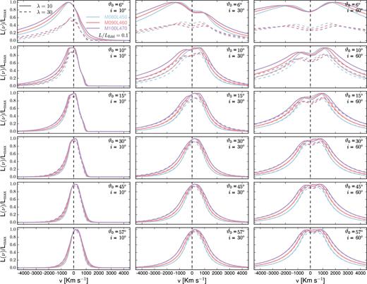
Normalized (with respect to the corresponding λ = 10 case profile) line luminosity versus velocity for several values of viewing and launch angles. Each panel shows the profiles for given launch and viewing angles. Along rows, launch angles are constant, and viewing angles increase from left to right. Only profiles corresponding to three viewing angles (i = 10°, 30°, 60°) are shown. The labels indicate log Mi and log Li, where Mi is the mass of the central BH in the corresponding simulation, in units of solar masses, and Li is the assumed luminosity in erg s−1. For example, M080L450 indicates log Mi = 8.0 and log Li = 45.0. This set of lines correspond to the case L/LEdd = 0.1.
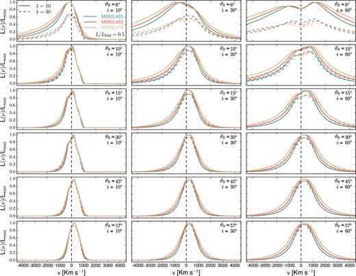
Normalized (with respect to the corresponding λ = 10 case profile) line luminosity versus velocity for several values of viewing and launch angles. Similar to Fig. 3, but for L/LEdd = 0.5.
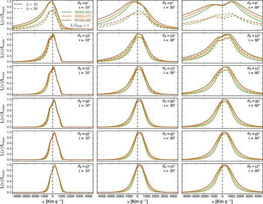
Normalized (with respect to the corresponding λ = 10 case profile) line luminosity versus velocity for several values of viewing and launch angles. Similar to Fig. 3, but for L/LEdd = 1.
Each panel of these figures includes the lines corresponding to fixed viewing and launch angles and luminosities, as described in the caption to Fig. 3. Solid and dashed lines correspond to λ = 10 and 30, respectively. The normalization is with respect to the corresponding λ = 10 case and only results corresponding to a subset of the viewing angles in the simulations are included. We postpone until Section 5 the discussion on how different λ values affect the results. The velocities in the x-axes represent velocities from the observer's point of view, therefore negative velocities correspond to blueshifts. The zero velocity, marked by a vertical dashed line in each panel, is the average of the two doublet wavelengths.
Within each panel, not only the profiles are broader with increasing mass and decreasing luminosity, but also the shift of the peak and the fractions of the flux blue- and redwards of the central velocity vary. For fixed ϑ0, the profiles are broader as the inclination angle increases. The dependence of the line-profile width on mass and luminosity can be seen by considering the Keplerian speed |$V_{\rm K} \sim \sqrt{M/r}$| and using equation (13) to express r ∼ M1/3L1/2, we find that VK ∼ M1/3L− 1/4. The profiles corresponding to any mass–luminosity combination have similar general behaviour and trends to the fiducial case, analysed in Paper I. For instance, all profiles have a certain degree of asymmetry that decreases with increasing inclination. As before, the blue wings change less than the red wings, so that as the inclination angle increases, the red wings become relatively stronger. Physically, the wind velocity depends on the launch angle, but the observer sees the fraction projected on to the LoS. However, as discussed in Paper I, in the framework of the present model, the actual angle to be considered is the angle ϑ at which a line launched with some ϑ0 crosses the base of the emitting region (when ϑ0 increases, so does ϑ). For any given combination of the two angles i and ϑ0, the projection of the velocity will be towards the observer on the fractions of the emitting region that satisfy the condition ϑ > i. The velocity relevant for producing the observed line profiles is the Doppler velocity, that includes a contribution from the rotational velocity. As ϑ increases, the rotational velocity becomes increasingly dominant, producing more symmetric profiles. For any launch angle, the relative importance of the receding term with respect to the approaching term increases with increasing viewing angle, but the effect is larger for smaller ϑ0.
The shape of a spectral line can be characterized by analysing the ratio S = FWHM/σl, where σl is the standard deviation of the line. For a Gaussian profile, |$S_{\rm {Gauss}} = 2 \sqrt{2 \ln (2)} \simeq 2.35$|, while S → 0 for Lorentzian and logarithmic profiles. For our results, we find minimum and mean S values ∼0.69 and ∼1.33, respectively.
Fig. 6 shows the distribution of the parameter S for our profiles as a function of two different line-width measures: FWHM in the right and σl in the left. The fact that most of our lines are below the SGauss value indicates that they have more prominent wings than a simple Gaussian profile. This is not surprising, as the dynamics is dominated by the turbulent plus thermal velocity.
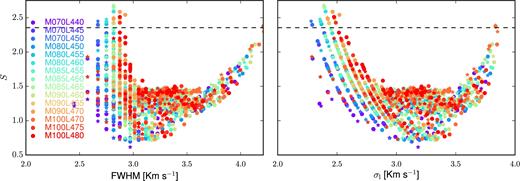
Line shape parameter, S versus FWHM (left) and S versus σl for all λ = 10 profiles, with S = FWHM/σl, where σl is the standard deviation of the line. The dashed line shown in both panels indicates |$S = S_{\rm {Gauss}} = 2 \sqrt{2 \ln (2)} \simeq 2.35$|. Labels follow the scheme laid out in the caption to Fig. 3.
4 FWHM STATISTICS
Here, we explore the FWHM of our profiles in relation to the luminosity of the sources and then consider the dispersion of this line-width characterization. Using the FWHM allows a fairly simple comparison to the observational data and constraints reported by Fine et al. (2010), who used interpercentile values (IPV) to characterise the line-widths, and an immediate possibility of extension to other works in the literature.
Fig. 7 shows the log (FWHM) of the line profiles from our simulations. Each panel corresponds to a given mass and luminosity and each colour, to a different launch angle, with solid and dashed lines used for the λ = 10 and λ = 30 cases, respectively. Here, we can see again that the results follow the expected behaviour of the FWHM with mass and luminosity, i.e. the FWHM increases with increasing mass and decreasing luminosity.
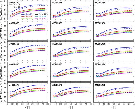
Profile FWHM versus inclination angle. Solid lines are λ = 10 cases, while λ = 30 cases are represented by dashed lines. Each panel corresponds to a different combination of mass and luminosity and each line represents results for a given launch angle.
Notably, for any given mass and luminosity (i.e. within a particular panel), the differences due to the angular momentum are almost independent of the launch angle, except for the lowest ϑ0 value. As mentioned, detailed discussion on this matter is placed in Section 5.
4.1 Luminosity–line-width plane
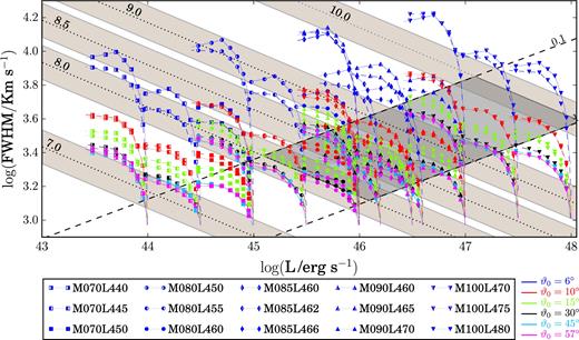
Similar to fig. 2 of Fine et al. (2010). The grey-shaded area corresponds approximately to the densest region in that figure. Note that the quantities in both axes differ from the ones used by Fine et al. (2010). In the x-axis, we used luminosities instead of absolute magnitudes and for the line-width measure, in the y-axis, we used FWHM instead of IPV. The dotted and dashed lines represent loci of constant mass and Eddington ratio, respectively, where the mass has been evaluated using equation (7) in VP06 (reproduced in equation 14). The shaded regions are bound by lines of constant log (Mi/M⊙) ± 0.2, where Mi is one of the mass values used in our simulations. Any point in the plane represents the result from a simulation with given mass, luminosity and launch and inclination angles. Each symbol corresponds to a mass–luminosity combination, and each colour (with the same scheme used in other figures), to a launch angle. For fixed ϑ0 the coloured solid lines join cases corresponding to different viewing angles. For any given mass–luminosity case, we see that results from the lowest ϑ0 values are consistently larger, for fixed i, that results from any other launch angle. Furthermore, the lower the launch angle, the larger the spread in log (FWHM) values.
The shaded regions are bound by lines of constant log (Mi) ± 0.2, where Mi is one of the mass values used in our simulations, in units of solar masses. While the sample standard deviation of the weighted average zero-point of their mass scaling relationships reported by VP06 is 0.36 dex, we used a smaller range around log Mi to avoid overlapping of regions belonging to two different such values. For each mass–luminosity combination, results corresponding to the same launch angle but different inclination are linked by solid lines, with the same colour scheme used in other figures.
The differences in luminosity from sources of intrinsic identical luminosities are attributable to the differences in viewing angle, because the observer sees a fraction that depends on the projection on the sky of the emitting region, so the x-axis is constructed by multiplying the assumed object's luminosity by the cosine of the inclination angle.
Note that if the black hole mass were estimated using equation (14), many of the results could not retrieve their original mass values. In general, the cases that seem best represented by the expression are in the range 8.0 ≲ log Mi ≲ 8.5, in particular for the largest viewing angles. For log Mi ∼ 9, fewer combinations, corresponding to the larger Eddington ratios, smaller ϑ0 and larger i, reproduce the original mass values, whereas log Mi ∼ 10, no combination can retrieve their true MBH. This is partly due to the fact that the expression given by VP06 does not include any angular dependency, although the issue is, in effect, analysed in their work. While the case of dependence on launch angle has not been studied, the influence of the viewing angle has been considered in several works (e.g.VP06; Collin et al. 2006; Decarli et al. 2010; Assef et al. 2011; Denney 2012). One way to compare the masses obtained by applying, VP06 equation (7) versus the objects’ true masses is to study, for given ϑ0, the mean of the ratio of the two quantities up to different imax values in a torus model. Fig. 9 shows normalized histograms of 〈log (MVP06/MTrue)〉, with the panels arranged according to the launch angle. The FWHM values are taken from the interpolated function. All histograms are skewed and their widths depend strongly on the launch angle. Note that the skewness direction also depends on this angle, and is positive for the smallest ϑ0 and becomes increasingly negative as the launch angle increases. In Fig. 10, we present the normalized histogram of the distribution of 〈log (MVP06/MTrue)〉 as function of imax for the whole set adopting a smooth torus model (discussed in more detail in Section 4.2).
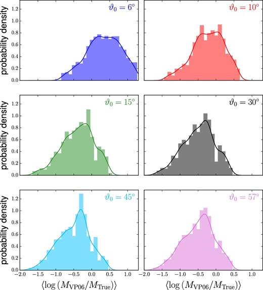
Normalized histograms of the quantity 〈log (MVP06/MTrue)〉, up to a set of imax values within a smooth torus model, for the different mass sets. Each panel corresponds to a given launching angle. The solid lines represent smooth histograms (kernel density estimation, KDE) over the same data. The skewness is positive in all cases, except the corresponding to |$\vartheta _0 = 6^\circ$|, and becomes increasingly negative as the launch angle increases.
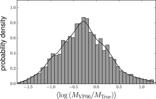
Normalized histograms of the quantity 〈log (MVP06/MTrue)〉 as a function of imax for all mass sets, no discriminating by launch angle or black hole mass.
Note that the correlation between FWHM and IPV has a non-negligible scatter, as can be seen from e.g. fig. A8 of Fine et al. (2010). Moreover, there is no direct conversion from one measure to the other, except for well-determined cases, such as a Gaussian curve, for which the relation is FWHM = 1.75 IPV. This degeneracy makes the comparison between our line-width versus luminosity with fig. 2 of Fine et al. (2010) not completely straightforward. A more direct comparison can be done with the results of Decarli et al. (2008), who reported a mean 〈FWHM〉 = 4030 ± 1200 km s−1from their sample. This value might be consistent with our findings, although it should be pointed out that their sample was much smaller than that of Fine et al. (2010).
4.2 Dispersion of log FWHM-smooth torus
Analogous to what we did in Paper I, we also analyse the FWHM of our line profiles applying the prescription of Fine et al. (2008, 2010), who constrained the possible viewing angles using geometrical models for the BLR and comparing the expected dispersion in line-widths to their observational data. Fig. 11 sketches the assumed geometry.
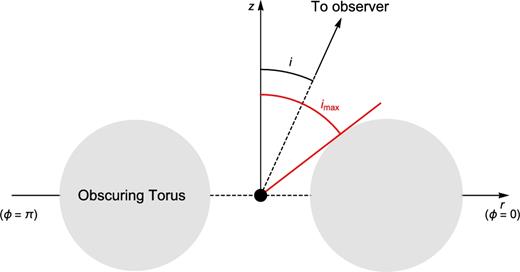
Torus geometry. The angle i is the observing angle to the AGN, and the opening angle imax assumed to be constrained by an obscuring torus.
Here, we perform the same calculations for each of the combinations of mass and luminosity. Thus, for each set of profiles obtained for different inclination angles i and launch angles, ϑ0 we study how the FWHMs are distributed with respect to i. For the C iv case that is of interest here, Fine et al. (2010) obtained an observational σf(imax) = 0.08 dex limit.
We show the dispersion of our line profile sets versus imax in Fig. 12. The panels are arranged as constant mass along rows and constant Eddington ratio along columns, and the black horizontal dashed line in each of them represents the Fine et al. (2010) constraint. Only dispersions that satisfy σf(imax) ≤ 0.08 dex are allowed, which imposes a constraint on the possible imax. In this test, the constraint on imax represents the torus half-opening angle that would yield a type 1 object. The solid and dashed lines correspond to λ = 10 and λ = 30 cases, respectively.
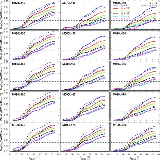
Standard deviation of the profile FWHM versus inclination angle. Each panel corresponds to a different combination of mass and luminosity and each line represent results for a given launch angle. The black horizontal dashed line corresponds to the Fine et al. (2010) 0.08 dex constraint.
The set of allowed imax changes from left to right, increasing as the Eddington ratio increases. From top to bottom, i.e. for constant Eddington ratio, the range of allowed imax values shrinks with increasing mass. These features are related to the torus geometry and its dependence on mass and luminosity and will be discussed below.
As shown in Paper I for the fiducial case, another way to visualize the constraining of the imax parameter is by making, for each mass–luminosity combination, contour plots of the corresponding σf(imax) as function of both ϑ0 and imax. In Fig. 13, we show such contour plots of the standard deviation of the profile FWHM versus launch and inclination angles for our set of masses and luminosities for the case λ = 10. The data are shown in the same arrangement as in Fig. 12.
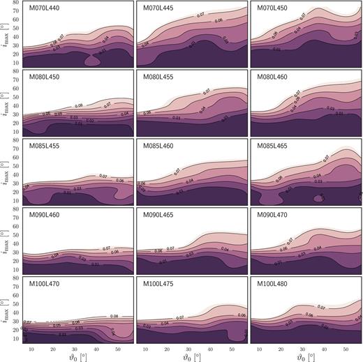
Contour plot of the standard deviation of the profile FWHM versus launch and maximum inclination angles, for the λ = 10 case. Only the contours within the region matching the Fine et al. (2010) results are shown. Each panel corresponds to a different combination of mass and luminosity, labelled according to the adopted convention, as described in the caption to Fig. 3.
Recall that the region allowed by the Fine et al. (2010) result is a measure of the torus opening angle and the torus is, in the standard model, the component that determines whether an object seen under a viewing angle i is type 1 or 2. As can be seen from Fig. 13, in the present framework, our upper limit on the half-opening angle of the torus of an AGN depends on both the mass and luminosity of the central engine.
If the broadening of the lines were only due to Keplerian motions modulated by the inclination dependence, the Fine et al. (2010) test would not differentiate among different mass–luminosity combinations, because that test analyses the dispersion of the logarithm of the line FWHMs rather than the FWHMs themselves. The fact that there are great differences in the allowed regions in the imax − ϑ0 plane for the different cases is a consequence of a more complex entanglement between the relevant parameters (mass, luminosity, viewing and launch angles, acceleration mechanism, etc.).
Looking along each row in Fig. 13 the mass is constant and the allowed regions in the imax − ϑ0 plane increase in size from left to right, as the Eddington ratio increases. We would like to link this to observational results other than those of Fine et al. (2010). By construction, increasing the allowed region implies the possibility that the torus opening angle measured from the axis also increases. In the scenario under consideration (fixed mass), that would imply that more luminous objects have a higher probability of being observed as type 1 than less luminous counterparts. That is, there could be more torus opening angle values under which a luminous object would be classified as type 1 than there are for fainter objects. Recent discussions in the literature suggest that this might the case. Elitzur et al. (2014) extended the analysis of Elitzur & Ho (2009) and confirmed the viability of a model where AGN broad-line emission follows an evolutionary sequence from type 1 to 2 as the accretion rate on to the central black hole is decreasing. The authors suggest that the (at least partially) controlling parameter of this spectral evolution and the torus opening angle is LBol/M2/3, that is only a function of L for the M = const case.
On the other hand, at fixed Eddington ratio (i.e. along a column in Fig. 13), the allowed region decreases from top to bottom, i.e. with increasing mass. The Elitzur et al. (2014) results could be interpreted as implying that under fixed Eddington ratio conditions the torus opening angle (measured from the axis) should increase with decreasing mass. That can be seen by rewriting the Elitzur et al. (2014) parameter in terms of the Eddington ratio as |$L_{\rm Bol} /M^{2/3} = \left(L_{\rm Bol} /M\right) M^{1/3} \propto \left(L_{\rm Bol} /L_{\rm Edd} \right) M^{1/3} = \dot{m} \, M^{1/3}$|. As mentioned, for the fixed Eddington ratio case, the results for our limits are opposite to Elitzur et al. (2014). However, when considering fixed mass, our results match those of Elitzur et al. (2014). An observational direct realization of such a case was discussed by LaMassa et al. (2015) as a plausible explanation for the ‘changing look’ quasar they discovered.
Note here that, in the case of Elitzur et al. (2014) framework, the decrement in observed broad lines originates in a decreasing accretion rate towards the central engine, which in turn decreases the outflow rate and the object's bolometric luminosity. At sufficiently low accretion rates, the BLR and the obscuring region are quenched, running out of fuel.
We can also analyse how our findings can be explained in the context of a popular parametrization of the BLR size and the vertical size of the torus that is related to its half-opening angle, σt. Some determinations of the vertical size of the torus (e.g. Simpson 2005) provide ht ∝ L1/4. We can, then, obtain a crude estimate of the BLR opening using (see e.g. Hönig & Beckert 2007) σt ∼ ht/RBLR ∼ L−1/4. Therefore, more luminous objects would have smaller torus openings (measured from the disc). This is in agreement both with our results (at M = const) and those of Elitzur et al. (2014).
The dependence of the torus height on luminosity is a modification suggested by Simpson (2005) to the model known as ‘receding torus’, proposed by Lawrence (1991), wherein the height of the torus is constant as a function of radius. As discussed in the recent review by Bianchi, Maiolino & Risaliti (2012), this dependence of the obscuring structure covering factor on the luminosity has been supported by many observational results, in different wavelengths. For instance, hard X-ray studies (e.g. Ueda et al. 2003; Akylas et al. 2006; Tozzi et al. 2006) and in the optical (e.g. Arshakian 2005; Simpson 2005; Polletta et al. 2008). Treister & Urry (2012); Alonso-Herrero et al. (2011) and more recently, Oh et al. (2015) also show results consistent with the receding torus model. Other authors, on the other hand, do not favour it. Lawrence & Elvis (2010), for instance, have questioned the validity of the above results, arguing that, at least in optical and IR-selected samples, such a luminosity dependence is an artefact due to the adopted definition of ‘obscured’ and to the inclusion of low excitation AGN.
4.3 Dispersion of log FWHM-clumpy torus
In clumpy torus models, the obscuring structure is discrete, consisting of optically thick clouds and the quasar is obscured when one such cloud is seen along the LoS. We start by briefly recalling the main characteristics of clumpy tori (e.g. Nenkova et al. 2008; Mor, Netzer & Elitzur 2009). In such a model, the torus is characterized by the inner radius of the cloud distribution (set to the dust sublimation radius, Rd, which depends on the grain properties and mixture) and six other parameters. These are the outer radius, Ro; the viewing angle i; the torus width parameter (analogous to its opening angle), σ; the mean number of clouds along a radial equatorial line, N0; the optical depth per cloud, τV (the same for all clouds in the configuration) and the power-law index of radial density profile, q, such that the number of clouds follows N(r) ∝ r−q. Note that the outer radius is often given through the alternative parameter Y = Ro/Rd. An implicit assumption is that the disc and torus are aligned.
Authors that support a clumpy rather than a smooth dust distribution torus (e.g. Hönig & Beckert 2007; Nenkova et al. 2008) argue that the decreasing fraction of type 2 objects at high luminosities discussed in Section 4.2 depends not only on the decreasing torus opening angle, but also on the decreasing N0. The torus ‘covering factor’ f2 is estimated by the fraction of type 2 sources in the total population (e.g. Lawrence & Elvis 2010) and is related to the torus half-opening angle according to |$f_2 = 1- \int _0^{\pi /2} P_{\rm esc}(i) \sin {i}\,{\rm d}i$|. For a smooth torus, this factor is given by f2 = sin σt but it is modified and becomes a function of the number of cloudets if a clumpy torus is considered.
In Fig. 14, we show the standard deviation of the profile FWHM versus launch angle obtained from our line profiles for the Nenkova et al. (2008) clumpy torus formulation. Note that as we have adopted the soft-edge case of the model, only |$i_{\rm {max}}=90^\circ$| is needed. Hence, the plots are curves and not contour levels. Each panel corresponds to a different combination of mass and luminosity and each line represents results for a different value of the torus model parameters σt and N0 adopted from the Mor et al. (2009) sample. The black horizontal dashed line is the Fine et al. (2010) 0.08 dex constraint.
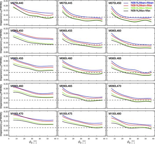
Standard deviation of the profile FWHM versus launch angle, using the Nenkova et al. (2008) clumpy torus prescription. The black horizontal dashed line corresponds to the Fine et al. (2010) 0.08 dex constraint. Each panel corresponds to a different combination of mass and luminosity and each line represent results for a given launch angle.
As in Fig. 13, the mass is constant along rows and the accretion rate is constant along columns. As in the smooth torus case, we find that the agreement (or lack thereof) with the observational constraint depends on the mass and the accretion rate separately, with better agreement (i.e. reached from a smaller ϑ0 angle) achieved for the lowest mass and larger Eddington ratio. Indeed, at the lowest |$\dot{m}$|, there is no combination of parameters that satisfies the condition imposed. Additionally, the curves corresponding to larger N0 cross the limiting line at smaller ϑ0. That is, our results favour denser structures.
5 COMPARING RESULTS FOR DIFFERENT λ VALUES
In previous sections, we have shown that the line profiles, and so their FWHMs and corresponding dispersions, depend only weakly on the dimensionless angular momentum parameter. Here, we discuss this result in terms of the velocity and magnetic fields governing the line formation in the framework of our model. Recall that, within the ideal MHD formalism of wind launching sketched in Section 2.1.2, the angular momentum l is constant along a field line (and so is its dimensionless version λ). Moreover, as also discussed in that section, in the EBS92 model (and, therefore in ours), the adopted free parameters are λ and ϑ0, while κ is related to λ by a non-linear correspondence, shown in equation (12). If we consider cases of equal masses and luminosities but different λ, and additionally assume same launch angles (i.e. same |$\xi ^{\prime }_0$| values) and density structures, we can see that the difference is due only to differences in the magnetic fields. In effect, equal masses imply equal Keplerian velocities, which in turn implies that the differences in the parametre k values can only be due to the magnetic field. Furthermore, equal masses also imply that the radial structure in the two cases are identical, so the difference in λ is only related to the poloidal variable ξ.
Comparing the profiles presented in Figs 3–5, it is evident that the differences in shape and line-width between results based on the two different λ values adopted depend on ϑ0 but very mildly (if at all) on the viewing angle. For i = const, the difference is maximum for the minimum adopted value of ϑ0 and becomes negligible as the parameter increases. For ϑ0 = const, the difference between profiles remain fairly constant along the whole range. There are a few departures, generally at the lowest ϑ0 and for the smallest i, but those do not invalidate the general behaviour.
Similarly, the shapes and FWHMs show maximum differences for ϑ0 = 6° and almost negligible for larger ϑs, as can be seen from Fig. 7. The dispersion of line-widths, plotted in Fig. 12, show also that the larger differences occur, in general, at smaller ϑ0 values, with a few cases where noticeable differences are seen at large ϑ0 angles.
The question is, then, why the results from the two different λ values seem to be more distinguishable for smaller ϑ0? To analyse the issue, we will exploit the independence of the differences between profiles on viewing angle mentioned above. Note that, for given M and L, these differences are also independent of ν. The above features allow us to choose convenient values for both frequency and i that will simplify the analysis. We therefore adopt ν = νD and i = 0° (although this particular viewing angle was not part of the simulations, the independence referred to allows this choice). Adopting ν = νD gives, replacing in equations (3) and (4), |$e_\nu = e_{\nu _{\rm D}}=1$| and |$x_\nu = x_{\nu _{\rm D}} = 0$|, respectively. Therefore, the optical depth, which is constructed using equations (2)–(4) as |$\tau _\nu = \tau \,\!e_\nu \,\!e^{-x_\nu ^2}$|, is simplified to |$\tau _\nu \!= \!\tau _{\nu _{\rm D}} \!= \! \tau$|. We also have VD(i = 0°) = Vpsin ϑ.
6 DISCUSSION
Considering the log L–log FWHM plane in Fig. 8 and the contour plots of Disp(log FWHM) in Fig. 13, we would like to assess which parameter(s), and in which direction(s), should be changed in future simulations to achieve better agreement with the observational results.
Note first that the angle imax used throughout this work is measured from the polar axis (i.e. it is the complementary to the angle σt = tan −1ht/rt defined above). The receding torus model posits that the imax parameter of more luminous objects is larger. Indeed, for constant mass our results permit that trend, although they hint that the torus opening angle of more luminous objects is smaller than that of fainter counterparts. But, as mentioned in Section 4.2, at fixed mass the trend is that reported by Elitzur et al. (2014), i.e. that the torus opening angle decreases with luminosity. These points suggest that our model is, in its general conception, adequate although some of the parameter choices have to be reviewed for it to better represent real cases.
For example, the tilt of the emitting region with respect to the equatorial plane was chosen to match that of MC97, which was in turn chosen based on a BAL quasar fraction of ∼0.1, a value that has been updated (Allen et al. 2011). More recent values put the BAL fraction as large as ∼0.25 of the quasar population, implying an emission region with a steeper slope. In such a case, the effective length over which the emission is obtained would increase and be at higher distances above the disc. This would affect both the velocities and their derivatives, thus affecting Q and the optical depth, ultimately modifying the FWHM of the line profiles, but perhaps not as much their shapes. Here, we recall that this slope can be a function of the radius, as opposed to the fixed value adopted in this work. Adopting a function that smoothly increases with radius (similar to the bowl-shaped BLR geometry in the model proposed by Goad et al. 2012) instead of a constant slope, would make the streamlines intercept the emission region at higher heights from the disc plane, which would produce broader profiles, and probably with more dispersion. A related description of the BLR structure, described as ‘nested rings’ geometry, was proposed by Mannucci, Salvati & Stanga (1992) and later reintroduced by Gaskell and collaborators (e.g. Gaskell, Goosmann & Klimek 2008; Gaskell 2009). Either of these geometries could provide a constraint to the families of possible curves to adopt as the base of the emission region.
The spatial profile of the density could be reviewed or adjusted, too. Here, we have to consider both the radial and the vertical structures, that are decoupled in the adopted model. As discussed in Section 2, the density structure in the radial direction is such that n(r) ∝ r−2, but a closer value to the corresponding Shakura & Sunyaev (1973) relevant accretion disc region would be a power-law exponent −3/2. Other possibilities involve changing the underlying disc model, adopting, e.g. a slim disc instead of the geometrically thin and optically thick disc of Shakura & Sunyaev (1973). Slim discs were developed in the pseudo-Newtonian limit by Abramowicz et al. (1988) and are more suitable for larger accretion rates (|$\dot{m} \gtrsim 0.3$|, e.g. Abramowicz & Fragile 2013).
In the z direction, the density drops off away from the base of the emission according to a half-Gaussian dependence, regulated by both the height and the thickness of the emission region. The former depends on the geometry of the region, discussed in the previous paragraph. Any modification to the latter should still ensure that it satisfies lem ≪ zem. The radial size of the line-emitting region, given by the ratio rmax/rmin, was fixed throughout this work. However, the amount of line shift and the degree of asymmetry of the line profiles are functions of it (e.g. Flohic et al. 2012). Therefore, it would be important to effectively study how this parameter affects the results.
The turbulent velocity has been chosen to be constant, but it also can depend on the radial coordinate. For instance, it has been shown that magnetorotational instability (MRI; Balbus & Hawley 1991) provides a plausible mechanism to develop turbulence and transport angular momentum in discs, due to their differential Keplerian rotation.
Changes in the adopted prescription of any (or all) of these parameters will lead to a different structure of the gas and its ionization and excitation states, in the disc and wind. For example, for most of their model cases MC97 and MC98 employed a (modified in the X-ray region) Mathews & Ferland (1987) SED, that is still very popular in the literature. Adopting a different SED would affect the ionization structure in the wind, but in a wind scenario there is no total freedom in choosing an alternative. A distribution too strong in X-rays compared with the UV portion may preclude the formation of a wind, because the gas is overionized before it can be accelerated. In such a case, the higher ionization lines, such as C iv, would instead be produced in the low-velocity gas, which is illuminated by a continuum that is now strong in the extreme UV and in the X-rays (Leighly 2004).
In Section 2.1.2, we mentioned that our work does not account for scattering effects. However, the importance of this process has been recently highlighted by Higginbottom et al. (2014) who, using Monte Carlo radiative transfer simulations, showed that including scattering of ionizing photons leads to a very high ionization parameter and modifies the outflow emission properties.
7 SUMMARY AND CONCLUSIONS
In this work, we have studied AGN BEL profiles with a model that combines an improved version of the accretion disc-wind model of MC97 with the hydromagnetic driving of EBS92. The dynamics of these self-similar MHD outflows is characterized by two parameters, e.g. the dimensionless angular momentum λ, and the wind-launch angle with respect to the disc plane ϑ0.
We have compared the dispersions in our model C iv line-width distributions to observational upper limits on that dispersion. Those limits translate to an upper limit to the half-opening angle of the putative torus feature that is part of the standard model describing the AGN phenomenon. To achieve this, we constructed contour plots of the dispersion of log (FWHM) in the ϑ0 − imax plane, capped with the Fine et al. (2010) observed upper limit dispersion, defining in this way a boundary line imax versus ϑ0, below which an object can be seen as type 1.
The maximum torus half-opening angle of about 47|$^\circ$| reported in Paper I has been corrected. That value was obtained based on an erroneous interpolation routine of the cloudy-generated source function points. The revised maximum torus half-opening angle is larger, about 75|$^\circ$|. In fact, the maximum torus half-opening angle is an increasing function of the wind launch angle ϑ0.
We extended the analysis presented in Paper I to consider a range of black hole masses and luminosities. In a similar manner to the approach adopted in the fiducial case, we computed, for different combinations of mass and luminosity of the central object within that range, line profiles corresponding to the same combinations of wind-launch and viewing angles used before. Additional series of model runs with different values of λ suggest that the profile line-widths and corresponding dispersions depend only mildly on this parameter.
We also found that many of the profile line characteristics, such as the FWHM, the (blue- or red-) shift with respect to the systemic velocity, and the degree of asymmetry, depend not only on the viewing angle (a parameter external to the object, depending on the orientation of the observer relative to the source), but also on the launch angle ϑ0, a parameter that is intrinsic to the object. Additionally, our results suggest that large values of ϑ0 are preferred.
The analysis of the luminosity–line-width relation showed that the black hole masses could not be recovered if the relation proposed by VP06 (reproduced in equation 14) is applied. While this discrepancy could be due to the FWHM of our line profiles, it would be worth evaluating if the inclusion of new empirical data from the literature supports the view that the expression needs to be reconsidered.
We then studied, for each case, the dispersion of log (FWHM) and imposed the observational results of Fine et al. (2010). Again, contour plots of the dispersion of log (FWHM) in the ϑ0 − imax plane, constrained with the Fine et al. (2010) results, were used to determine the torus half-opening angle appropriate for each case. The picture that emerged is that the dispersion of the line-width depends on both the mass of the central object and the Eddington ratio at which it is fed. At fixed mass, the maximum allowed torus half-opening angle (measured from the axis) increases with increasing Eddington ratio (equivalent, under the fixed mass condition, to increasing luminosity). That can be interpreted as objects with larger accretion rates having a higher probability of being observed as type 1 AGN than those fed at a lower rate. At fixed Eddington ratio, the probability that an object will be seen as type 1 decreases with increasing mass. But the time-scales for mass changes due to accretion are large enough for any particular system to be considered as constant mass, and, as mentioned above, in that scenario our results are in agreement with the observational report of Elitzur et al. (2014).
A clumpy torus was also analysed. The limiting viewing angle to integrate over this was always 90°, as opposed to the differential imax that was used in the putative smooth torus case. Except for this difference, this alternative obscuring structure yielded similar constraints to those obtained with the traditional torus. Moreover, the results favour denser structures.
Ultimately, this work links theory with observational results, by imposing an observational constraint to the distribution of a property of the emission lines emerging from the BLR. The BLR is modelled through a physically well-motivated wind description and the observational constraint on the dispersion of the line-width distribution allows it to be translated into a constraint on the geometry of the obscuring structure that is invoked to explain the type 1/type 2 dichotomy among AGNs.
Acknowledgments
LSC and PBH acknowledge support from NSERC. The authors would like to thank the anonymous referee for very helpful comments and suggestions.
