Gravitational instability of filamentary molecular clouds, including ambipolar diffusion

Hosseinirad, Mohammad; Naficy, Kazem; Abbassi, Shahram; Roshan, Mahmood

doi:10.1093/mnras/stw2820

Abstract

The gravitational instability of a filamentary molecular cloud in non-ideal magnetohydrodynamics is investigated. The filament is assumed to be in hydrostatic equilibrium. We add the effect of ambipolar diffusion to the filament which is threaded by an initial uniform axial magnetic field along its axis. We write down the fluid equations in cylindrical coordinates and perform linear perturbation analysis. We integrate the resultant differential equations and then derive the numerical dispersion relation. We find that a more efficient ambipolar diffusion leads to an enhancement of the growth of the most unstable mode, and to the increase of the fragmentation scale of the filament.

diffusion, instabilities, MHD, methods: numerical, ISM: clouds

1 INTRODUCTION

Finding a reliable description of star formation has been one of the pivotal challenges of astrophysics for decades. Having such a model for star formation which involves many diverse physical phenomena would provide invaluable information to understand the evolution of galactic structures, star clusters, binary stars and even the formation of planets. It has been long established that stars form from collapsed dense molecular cloud (MC) cores [see Klessen, Burkert & Bate (1998), Dib et al. (2007), McKee & Ostriker (2007) and Padoan, Haugbølle & Nordlund (2014)]. These cores are substantially denser than their parents so they collapse faster. Nevertheless, once these fragments turn into stars they start to affect the surrounding (by radiation, winds or supernova explosions) preventing it from collapsing and forming stars. Generally it should be possible to derive a model that follows it from the scale of the largest self-gravitating clouds, the giant molecular clouds (GMCs; ∼100 pc), to the scale of protostars (∼10⁻⁵ pc); while this is not possible in direct hydrodynamic simulations due to resolution limits, it can be studied approximately in analytic and semi-analytic models.

Filamentary structures are quite commonly found in the interstellar medium. Recent high angular resolution and signal-to-noise ratio of dust imaging with the Herschel Space Observatory have revealed the filamentary nature of the dense MCs in unprecedented details (André et al. 2010; Molinari et al. 2010). Consequently it has been suggested that such filamentary structures likely play a key role in the star formation process. Filaments are also ubiquitously observed in numerical simulations of supersonic turbulence in MCs and of the interstellar medium (e.g. Klessen et al. 1998; Dib & Burkert 2005; Ntormousi et al. 2016). These filamentary structures exhibit a large degree of sub-structures of their own (such as clumps and cores). André et al. (2010, 2014) proposed that turbulence-driven filaments are maybe the first stage of star formation. Given the widespread interest in the filamentary clouds structure and evolution and their key role in star formation, it is worth to examine the stability properties of the filaments in their realistic setting.

It is now accepted that a magnetic field plays a significant role on the dynamics of MCs and consequently on the star formation process (Heiles et al. 1993; McKee et al. 1993; Dib et al. 2010). Large-scale magnetic fields can limit compression in interstellar shocks that form cores and filaments, while the local magnetic field within cores and filaments can prevent collapse if it is large enough (Mouschovias & Spitzer 1976). We know that magnetic fields are coupled with ionized particles, while the gas in the GMCs and their substructures such as filaments are mostly neutral or partially ionized. Mestel & Spitzer (1956) proposed a process, ambipolar diffusion, that allows charged particles to drift relative to the neutrals, with a drag force proportional to the collision rate. Also ambipolar diffusion leads to the dissipation of magnetic field as well as to driving the system into force-free states (Zweibel & Brandenburg 1997). Consequently, ambipolar diffusion will modify effectively the dynamical role of the magnetic field on the gas, and plays a key role in the star formation process.

It has been proposed that quasi-static ambipolar diffusion is the main mechanism for pre-stellar core formation. However, in this quasi-static evolution model (Mouschovias & Ciolek 1999; Ciolek & Basu 2001) the pre-stellar lifetime is considerably larger than most accepted values (2–5 free fall time-scales; Ward-Thompson et al. 2007). It is now generally recognized that, due to pervasive supersonic nature of flows in GMCs, core formation is not likely to be quasi-static. In a realistic picture for star formation, we need to take both the ambipolar diffusion and supersonic turbulence of the gas into account.

Gehman et al. (1996a) studied the linear evolution of small perturbations of self-gravitating filamentary clouds. They consider wave-like perturbations to a non-uniform filament. Due to the non-thermal nature of interstellar gas, which is confirmed observationally, they modified their equation by adding a term that attempts to model the turbulence. They numerically determined the dispersion relation and consequently the form of perturbations in the regimes of gravitational instability. In their subsequent work, in the framework of the ideal magnetohydrodynamics (MHD) theory, they added a uniform axial magnetic field and concluded that the existence of fastest growing modes and their characteristics highly depend on the amount of turbulence and the strength of the magnetic field (Gehman, Adams & Watkins 1996b).

The purpose of this paper is to add the effect of the ambipolar diffusion in the gravitational instability of filamentary MCs with magnetic field using non-ideal MHD. The outline of this article is as follows: in Section 2, we present the basic MHD equations, which include the induction equation with an ambipolar diffusion term. We also describe the physical assumptions that are applied to the system. The unperturbed state of the system is introduced in Section 3. In Section 4, we perform linear perturbation analysis and then describe briefly the boundary conditions (BCs) and numerical method which are used to solve the perturbed equations in Sections 5 and 6, respectively. We express the results in Section 7. In Section 8, we discuss our findings and finally, we summarize our conclusions in Section 9.

2 MHD EQUATIONS WITH AD

If the degree of ionization in a medium is very low, the force associated with the pressure gradient of the ions and their gravitational force could be neglected in comparison with the Lorentz and ion-neutral drag force. Accordingly, the Lorentz force and the drag force exerted by the neutrals on the ions could virtually balance each other. The equations of MHD in this so-called strong coupling approximation (Shu 1983) with self-gravity and AD term are as follows:

\begin{equation} \frac{\mathrm{\partial} \, \rho }{\mathrm{\partial} t} + \nabla \cdot \left(\rho \boldsymbol {u}\right) = 0, \end{equation}

(1)

\begin{equation} \rho \frac{\mathrm{\partial} \, \boldsymbol {u}}{\mathrm{\partial} t} + \rho \left(\boldsymbol {u}\cdot \nabla \right) \boldsymbol {u} + \nabla p + \rho \nabla \psi - \frac{1}{4\pi }\left(\nabla \times \boldsymbol {B}\right)\times {\bf \boldsymbol {B}} = 0, \end{equation}

(2)

\begin{eqnarray} \frac{\mathrm{\partial} \, {\bf \boldsymbol {B}}}{\mathrm{\partial} t} + \nabla \times \left({\bf \boldsymbol {B}}\times \boldsymbol {u}\right) - \nabla \times \lbrace [\eta _A (\nabla \times {\bf \boldsymbol {B}})\times {\bf \boldsymbol {B}}]\times {\bf \boldsymbol {B}} \rbrace = 0, \end{eqnarray}

(3)

\begin{equation} \nabla ^{2}\psi = 4\pi G \rho , \end{equation}

(4)

where ρ is the neutral gas density, |$\boldsymbol {u}$| is the fluid velocity, p is the pressure, ψ is the gravitational potential and |${\bf \boldsymbol {B}}$| is the magnetic field strength, whereas η_A is the AD coefficient indicated by

\begin{equation} \eta _A = \frac{1}{4\pi \gamma \rho _{\rm i} \rho } \end{equation}

(5)

(Shu, Adams & Lizano 1970), where ρ_i and γ are the ions density and the drag coefficient, respectively. Draine, Roberge & Dalgarno (1983) proposed the value of γ = 3.5 × 10¹³ cm³ g⁻¹ s⁻¹. Due to the cosmic radiation, MC are partially ionized. Elmegreen (1979) showed that one could approximate the relation between ions and neutrals density as

\begin{equation} \rho _{\rm i} = C \rho ^{1/2}, \end{equation}

(6)

where C is a constant equals to C = 3 × 10⁻¹⁶ cm^−3/2 g^1/2. So the equation (5) can be recast as

\begin{equation} \eta _A = \frac{1}{4\pi \gamma C \rho ^{3/2}} = \frac{1}{4\pi \alpha \rho ^{3/2}}, \end{equation}

(7)

where α is a substitution for γC and equals to α = 10.5 × 10⁻³ cm^3/2 g^−1/2 s⁻¹. These assumptions lead to a fractional ionization of n_i/n_n ∼ 10⁻⁷ for n_n ∼ 10⁴ cm⁻³, that is completely centred within 10⁻⁶ to 10⁻⁸ of observation of MC cores. By making the equations dimensionless, α and η_A become ≃11.465 and ≃0.007ρ^−3/2, respectively (see Section A). The aforementioned fluid equations, are closed by addition of one equation of state, which is considered here to be isothermal, i.e.

\begin{equation} p=P(\rho )=c_{\rm s}^2 \rho , \end{equation}

(8)

and, where c_s is the isothermal sound speed which is about 0.2 km s⁻¹ for an MC with temperature of 10 K and mean molecular weight of μ = 2.36. The above values for the number density and sound speed, will give the value of ∼0.7 for a typical MC threaded by a magnetic field of 10 μG.

3 UNPERTURBED STATE

The unperturbed fluid is supposed to be in the hydrostatic equilibrium state (⁠|$\boldsymbol {u}$| = 0). We make the assumption that the initial magnetic field does not have any role in stability of the filament. Therefore the density and gravitational potential profiles of the filament have analytical solutions (Stodólkiewicz 1963; Ostriker 1964) and could be written in cylindrical coordinates (r, Φ, z) as

\begin{equation} \rho (r)=\rho _{\rm c} \left(1+\frac{r^2}{8H^2}\right)^{-2} \end{equation}

(9)

and

\begin{equation} \psi (r)=2\ln \left(1+\frac{r^2}{8H^2}\right), \end{equation}

(10)

where ρ_c is the central density and H is a radial scale height of

\begin{eqnarray} H=\frac{1}{\sqrt{4\pi G}}\left( \frac{c_{\rm s}}{0.2\ {\rm km s}^{-1}}\right) \left( \frac{4\times 10^{-20}{\rm g cm}^{-3}}{\rho _{\rm c}}\right)^{1/2} \simeq 0.035\ {\rm pc}, \nonumber\\ \end{eqnarray}

(11)

whereas G is the gravitational constant. Note that although the radius of the filament extends to the infinity, the mass per unit length has a finite value of

\begin{equation} \frac{M}{l}=16.4\left(\frac{T}{10\ {\rm K}}\right)\ {\rm M}_{\odot }\ {\rm pc}^{-1}. \end{equation}

(12)

The initial magnetic field is taken to be uniform, with an axial component

\begin{equation} {\bf \boldsymbol {B}_0}=B_0 \boldsymbol {\hat{z}} \end{equation}

(13)

and we suppose that it does not contribute to the system equilibrium. This in turn guaranties that AD does not affect the initial steady state.

4 LINEAR PERTURBATION ANALYSIS

In the following, we write all the equations in dimensionless units by changing the quantities (see Appendix A for details). Unperturbed and perturbed quantities are denoted by subscript ‘0’ and ‘1’, respectively. We take η_A as a constant. This will ease the calculations as well as let us discuss the effect of AD more clearly.¹

If we disturb the equations (1)– (4) by addition of small perturbations (shown with subscript 1), they could be written to the first order as:

\begin{equation} \frac{\mathrm{\partial} \, \rho _{1}}{\mathrm{\partial} t} + \nabla \rho _0\cdot p{\bf \boldsymbol {u}}_1 + \rho _0\nabla\cdot p {\bf \boldsymbol {u}}_1=0, \end{equation}

(14)

\begin{equation} \rho _{0}\frac{\mathrm{\partial} \, {\bf \boldsymbol {u}}_{1}}{\mathrm{\partial} t} + \nabla p_{1} + \rho _{0}\nabla \psi _{1} + \rho _{1}\nabla \psi _{0} - \left(\nabla \times {\bf \boldsymbol {B}}_1\right)\times {\bf \boldsymbol {B}}_0 = 0, \end{equation}

(15)

\begin{eqnarray} &&{ \frac{\mathrm{\partial} {\bf \boldsymbol {B}}_{1}}{\mathrm{\partial} t} + \nabla \times \left({\bf \boldsymbol {B}}_{0}\times {\bf \boldsymbol {u}}_{1}\right) -\eta _A\nabla \times \lbrace [(\nabla \times {\bf \boldsymbol {B}}_1)\times {\bf \boldsymbol {B}}_0]\times {\bf \boldsymbol {B}}_0 \rbrace = 0}\nonumber\\ \end{eqnarray}

(16)

and

\begin{equation} \nabla ^{2}\psi _{1} = \rho _{1}. \end{equation}

(17)

The equation of state is assumed to be isothermal, so the pressure perturbation could be written as follows:

\begin{equation} p_1=P^{\prime }(\rho _0)\rho _1. \end{equation}

(18)

The linear property of the equations, allows us to decompose the perturbations to their Fourier modes as

\begin{equation} \left( \begin{array}{c}\rho _{1}(\boldsymbol {x}, t) \\ {\bf \boldsymbol {u}}_{1}({\bf \boldsymbol {x}}, t) \\ {\bf \boldsymbol {B}}_{1}(\boldsymbol {x}, t) \\ \psi _{1}(\boldsymbol {x}, t) \end{array}\right) = \Re \left[ \ \left( \begin{array}{c}f(r) \\ {\bf \boldsymbol {v}}(r) \\ {\bf \boldsymbol {b}}(r) \\ \phi (r) \end{array}\right) \exp {({\rm i}kz-{\rm i}\omega t)} \right]\!\!, \end{equation}

(19)

where ω is the angular frequency and k is the vertical wavenumber, whereas f(r), |${\bf \boldsymbol {v}}(r)$|⁠, |${\bf \boldsymbol {b}}(r)$| and ϕ(r) are the amplitudes of density, velocity, magnetic field and gravitational potential disturbances, respectively. We restrict ourselves to the study of the axisymmetric non-propagating evanescent unstable modes for which iω is a real negative number. After some vector and algebraic manipulation, the complete set of equations which must be solved are yielded as follows:

\begin{eqnarray} &&{ -\rho _0 w + fP^{\prime \prime }\frac{{\rm d} \rho _0}{{\rm d}r} + P^{\prime }\frac{{\rm d} f}{{\rm d}r}+\rho _0\frac{{\rm d} \phi }{{\rm d}r}+f\frac{{\rm d} \psi _0}{{\rm d}r}} \nonumber \\ &&{-\, \left(\frac{B_0^3k^2\eta _A}{\eta _A B_0^2k^2+\Omega }\right)\frac{{\rm d} b_z}{{\rm d}r}-\frac{B_0^2k^2w}{\Omega (\eta _A B_0^2k^2+\Omega )}} \nonumber \\ &&{ +\, B_0\frac{{\rm d} b_z}{{\rm d}r}=0,} \end{eqnarray}

(20)

\begin{eqnarray} r\rho _0\frac{{\rm d} w}{{\rm d}r}+\rho _0w+r(-\Omega ^2-k^2P^{\prime })f-rk^2\rho _0\phi +rw\frac{{\rm d} \rho _0}{{\rm d}r}=0,\nonumber\\ \end{eqnarray}

(21)

\begin{eqnarray} &&{ -\eta _A B_0^2\bigg (b_zk^2r-r(\frac{d^2b_z}{dr^2})-\frac{{\rm d} b_z}{{\rm d}r}\bigg )-\Omega b_z r }\nonumber \\ &&{ - B_0r\bigg (\frac{-\Omega f}{\rho _0}-k^2\frac{\phi }{\Omega }-k^2\frac{fP^{\prime }}{\Omega \rho _0}+\frac{w}{\Omega \rho _0}\frac{{\rm d} \rho _0}{{\rm d}r}\bigg )=0} \end{eqnarray}

(22)

and

\begin{equation} r\frac{{\rm d}^2\phi }{{\rm d}r^2}+\frac{{\rm d}\phi }{{\rm d}r}-rk^2\phi -rf=0, \end{equation}

(23)

where we substitute iωv_r as w and iω as −Ω. This system of four coupled ordinary differential equations (ODEs) can be converted to seven first-order ODEs. In this set of equations, we treat k as an eigenvalue and Ω as a constant parameter. This constitutes a two-point boundary value problem (BVP) with one eigenvalue.

5 BOUNDARY CONDITIONS

Equations (20) and (23) must be supplied with seven BCs to be solved. Axial symmetry demands that the radial components of the velocity and all forces must vanish on the axis of symmetry. Furthermore, as the equations are linear, another BC can be constrained by setting one of the dependent variables to an arbitrary value on the axis of the symmetry. We choose the density perturbation amplitude and give it the value of 1. So, we have four BCs on the filament axis that are

\begin{eqnarray} f=1,\quad \frac{{\rm d}\phi }{{\rm d}r}=0,\quad w=0,\quad \frac{{\rm d}b_z}{{\rm d}r}=0 \quad {\rm at}\quad r=0. \end{eqnarray}

(24)

Moreover, by imposing an evanescent condition, all the dependent variables and their radial derivatives have to vanish at infinity. So the remaining three BCs could be taken into account as

\begin{eqnarray} f=0,\quad w=0, \quad \frac{{\rm d}b_z}{{\rm d}r}=0 \quad {\rm at} \quad r=\infty . \end{eqnarray}

(25)

6 NUMERICAL METHOD

Several different methods exist to solve two-point BVPs. We use a Newton–Raphson–Kantorovich relaxation algorithm (Garaud 2001). The algorithm, uses the second-order finite-difference method to discretize the system of ODEs as well as BCs over a mesh grid. The resultant system of linear algebraic equations is then solved by inverting the matrix of coefficients. This procedure is iterated while an error-threshold test is performed after each iteration until the solutions are converged. The reader can find more details of the algorithm in Garaud (2001).

We implemented this algorithm by choosing a computational interval between r = 0 and 50. This interval was spanned with 2000 equally spaced mesh grid.

7 RESULTS

By solving the system of ODEs, a numerical dispersion relation for the system could be computed. At first, the results of Gehman et al. (1996b) for different magnetic field strength of B, are successfully re-produced by using an approach like theirs. These results are used as a guess for the new system of ODEs which includes the effect of AD. We examined, various values for the magnetic field strength B and AD coefficient η_A to comprehend how the dispersion relation (specially the fastest growing mode) could be affected.

There exist four eigenfunctions f, ϕ, v_r andb_z related to each point on the dispersion relation curve when the AD term is added (without AD, b_z as well as its derivative can be obtained algebraically, so the number of eigenfunctions is limited to three). In Fig. 1, the eigenfunctions of the fastest growing mode are depicted for B = 0.1, B = 1 and B = 10 each in three diffusivity regimes i.e. η_A = 0, 10 and 10⁴. The computed eigenfunctions when the magnetic field and in consequence AD are absent (pure Jeans instability) are also represented for comparison. From this figure, one can see that the amplitude of density perturbation f has generally the same shape in all of B and η_A values. Just in strong magnetic field, it is a little wider which by addition of AD it tends to come back to the state in which no magnetic field is present. The v_r eigenfunction is more prone to change with B alteration. Strong magnetic field is able to effectively damp the radial-velocity perturbation. This is expected since stronger magnetic field in the z direction will lead to stronger magnetic force against the radial motion of the ions.

Figure 1.

The eigenfunctions of the fastest growing mode in different magnetic field strength. The thick solid, dashed and dotted lines represent different η_A values of 0, 10 and 10⁴, respectively. For comparison, the eigenfunctions when magnetic field is not present are also depicted using thin solid black lines.

Open in new tab Download slide

Here, AD is also able to return the radial velocity to the case of no magnetic field more effectively. The treatment of ϕ gravitational potential eigenfunction is very much like that of density one. The AD influence is again to revert the system modes to the original state. In other words, AD suppresses the magnetic field effects and forces the system to respond against axisymmetric perturbations like a system in which there is no magnetic field. This fact is somehow surprising since one may naturally expect that increasing the AD coefficient η_A would highlight the existence of the magnetic field in the system instead of hiding its presence. Mathematically, one may conclude that large η_A makes the |$\left(\nabla \times {\bf \boldsymbol {B}}_1\right)\times {\bf \boldsymbol {B}}_0$| term in equation (16) small compared to other terms. This point gets more clear by noting the response of b_z to changes in η_A in the bottom panels of Fig. 1. It is evident that increasing the η_A coefficient strongly damps b_z and forces it to vanish. In this case, the last term in equation (16) would be straightforwardly very small. We will show that increasing η_A apparently hides the magnetic field effects on the eigenfunctions, but increases the growth rate of unstable perturbations. Furthermore, the perturbation of the gravitational potential, i.e. ϕ(r), has also been illustrated in Fig. 1. As expected, ϕ(r) similar to f(r) is not too sensitive to the AD coefficient.

Fig. 2 shows the dispersion relations for a sample of three selected magnetic field strengths, namely B = 0.1, B = 1 and B = 10. When η_A = 0, the magnetic field is the only agent that affects the propagation of disturbances by improving the stability of the filament. In these cases our results agree very well with previous studies [see e.g. Chandrasekhar & Fermi (1953), Ostriker (1964), Nagasawa (1987) and Gehman et al. (1996b)].

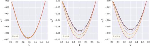
Dispersion relation for the filament for indicated B. In each figure, the horizontal axis is the wavenumber k and the vertical axis is ω2 that are normalized in the units of (4πGρc)1/2/cs and 4πGρc, respectively. Each dashed line demonstrates different ηA value from top to bottom as 0.01, 0.1, 1,10, 102, 103 and 104. The solid-red line represents dispersion relation for the case in which ηA = 0.

Figure 2.

Dispersion relation for the filament for indicated B. In each figure, the horizontal axis is the wavenumber k and the vertical axis is ω² that are normalized in the units of (4πGρ_c)^1/2/c_s and 4πGρ_c, respectively. Each dashed line demonstrates different η_A value from top to bottom as 0.01, 0.1, 1,10, 10², 10³ and 10⁴. The solid-red line represents dispersion relation for the case in which η_A = 0.

Open in new tab Download slide

However, the addition of AD to the physics of the problem, changes the response of the filament to the disturbances. As expected, in the weakest magnetic field (left-hand panel in Fig. 2), AD is not sufficiently efficient to change the shape of the dispersion relation even in very strong diffusion regime, just the growth rate of the fastest growing mode (i.e. the largest |ω²|) has increased fairly and also shifted towards smaller wavenumbers. For a stronger magnetic field B = 1 (central panel), lower η_A values, i.e. 0.01 and 0.1, are still almost ineffective. But for a larger value of η_A ≥ 1, the growth rate of the unstable modes increases in a tangible manner. More specifically the growth rate of the most unstable mode increases significantly. This effect is more pronounced when η_A = 10 and totally recognizable for η_A = 10², 10³ and 10⁴. It is also worth mentioning that AD increases the most unstable wavelength but keeps the spectrum of the unstable wavelengths constant. In other words AD does not extend the instability interval. This interval in Fig. 2 is 0 < k < 0.57. In this sense, one may conclude that AD does not make the system more unstable, and just increases the instability growth rate.

The right-hand panel in Fig. 2 illustrates this situation when B = 10. In this case, the previous story is repeated. Though when diffusion is absent the fastest growing mode is a few smaller, as η_A gets larger, the fastest growing mode becomes smaller. Another point that one could see simply is that the critical wavenumber remains constant regardless of the B and η_A values. It is instructive to mention that Gehman et al. (1996b) showed that a magnetic field stronger than B ≃ 2 is not able to further destabilize the filament. Fig. 3 depicts that in an inverse picture, this is also the case for very large η_A quantities. (see also Fig. 4).

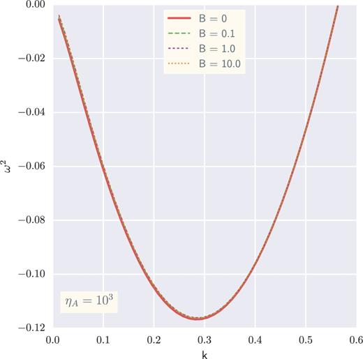
Comparison between B = 0.1, 1 and 10 in the strong AD regime ηA = 100. ω2 and k are normalized as Fig. 2. The solid-red curve represents dispersion relation for the case in which B = 0

Figure 3.

Comparison between B = 0.1, 1 and 10 in the strong AD regime η_A = 100. ω² and k are normalized as Fig. 2. The solid-red curve represents dispersion relation for the case in which B = 0

Open in new tab Download slide

Figure 4.

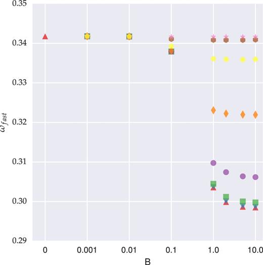
The fastest growing mode versus magnetic field strength. ω_fast and B are normalized in units of (4πGρ_c)^1/2 and (4πρ_c)^1/2c_s, respectively. Markers from top to bottom demonstrate different η_A values as 10⁴ (star), 10³ (hexagon), 10² (pentagon), 10 (diamond), 1 (circle), 10⁻¹ (square), 10⁻² (upside down triangle) and 0 (triangle). When B = 0, η_A has the only value of 0.

Open in new tab Download slide

To elaborate on the dependence of the fastest growing mode on B and η_A, a high-order polynomial is fitted on the calculated dispersion relation points. Fig. 4 represents the result. For magnetic fields B ≤ 0.01, even very large η_A values are not able to change the picture. The fastest growing mode remains unchanged. When B = 0.1, scaling up AD makes a little reduction in the fastest growing mode. In stronger magnetic field regime (B ≥ 1), increasing AD makes a sharp decline in the fastest growing mode values. Here, it is clearly visible that the stabilizing effect of magnetic field could be negated by AD.

Gravitationally unstable MC are fragmented most probably at the most rapid propagating mode. This means it is the wavelength of the fastest growing mode (λ_fast) which signifies a value for fragmentation length-scale of the filament. Axial magnetic field could reduce this length-scale by moving k_fast = 2π/λ_fast to some larger values (Gehman et al. 1996b). Fig. 5 shows that this phenomenon could be weakened by the addition of AD effect. As for an isothermal filament fragmentation mass scale is M_frag = 8πλ_fast (Gehman et al. 1996b), AD could also increase this mass scale.

Figure 5.

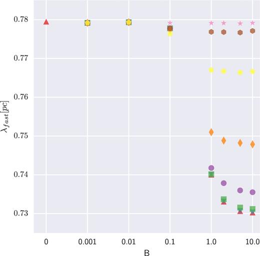
The length-scale of fragmentation versus magnetic field strength. B is normalized as Fig. 4. B = 1 corresponds with ∼14.3 μG. λ_fast is in the unit of pc. Markers from top to bottom demonstrate different η_A values as 10⁴ (star), 10³ (hexagon), 10² (pentagon),10 (diamond), 1 (circle), 10⁻¹ (square), 10⁻² (upside down triangle) and 0 (triangle). When B = 0, η_A has the only value of 0.

Open in new tab Download slide

Fig. 6 demonstrates cross-section of the filament for the fastest growing mode when AD is not present. The overall pattern of velocity and total (initial + perturbed) magnetic field (when existing) are overlaid on the total density background. The axial structure of the magnetic field is preserved even in the weak magnetic field. For velocity, it is a little different. It tends to twist towards the centre of filament as the distance increases. Rising B value, attenuates this treatment and makes velocity field to lay along the filament vertical axis. Fig. 7 is similar to its previous counterpart. It shows the situation when AD is contributing to the structure of the filament. AD can restore the twisted pattern of velocity field observed in absence of the magnetic field. The axial shape of the magnetic field still remains unchanged.

Figure 6.

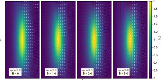
Cross-section of the filament without AD effect in different magnetic field strength (from left to right B = 0, 1, 2 and 5). White and red (when present) arrows indicate the total velocity and magnetic vector field overlaid on background of total density for the fastest growing mode.

Open in new tab Download slide

Figure 7.

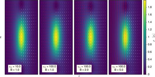
Cross-section of the filament with AD effect (η_A=10 or 100) in different magnetic field strength (from left to right B = 1, 1, 2 and 5). White and red (when present) arrows indicate the total velocity and magnetic vector field overlaid on background of total density for the fastest growing mode.

Open in new tab Download slide

8 DISCUSSION

8.1 The time- and length-scale of fragmentation

Pertaining to the fastest growing mode, two important scales are the time-scale and length-scale of fragmentation. By increasing the AD coefficient, the coupling between neutrals and ions becomes more and more fragile. This means that the support by the magnetic field becomes less and less efficient until it becomes entirely inefficient and neutrals are no longer tied to the magnetic field lines at all. In other words, existence of the AD, moves the system towards Jeans instability. This fact can be seen in Figs 4 and 5. Fig. 4 shows that for all the magnetic field strengths, increasing more and more the AD effect leads all the fastest growth rates to converge to a maximum value of around

\begin{equation} |\omega |^2_{{\rm max}}=0.117, \end{equation}

(26)

which is equivalent to a minimum growth time-scale of

\begin{equation} \tau _{{\rm min}}\simeq 3.1\ {{\rm Myr}}. \end{equation}

(27)

One should note that by equation (27), the minimum growth time-scale is roughly comparable or even greater than the typical lifetime of MCs harbouring these filaments (e.g. Ward-Thompson et al. 2007). As it is pointed out in the Introduction, the turbulent flow in the interstellar medium and GMCs, could accelerate the diffusion of the magnetic field (Fatuzzo & Adams 2002; Kim & Diamond 2002; Zweibel 2002; Heitsch et al. 2004; Li, McKee & Klein 2012). Kudoh & Basu (2011) in a three-dimensional simulation of sub-critical sheet-like MC showed that the supersonic velocity perturbation could accelerate the AD time by an order of magnitude. In a very recent work, Burge et al. (2016) have shown that by addition of a decaying turbulent velocity field, the AD collapse time of a filament could be decreased. It is worth noting that Gehman et al. (1996a,b) also derived the dispersion relations of filaments with equations of state that are softer than isothermal as a representative for turbulent fluid and showed that it can decrease the minimum growth time.

Moreover, by Fig. 5, one could simply find that there is also a maximum value for the most unstable wavelength around

\begin{equation} (\lambda _{{\rm fast}})_{{\rm max}}=0.779\ {{\rm pc}}. \end{equation}

(28)

This length-scale indeed is the most unstable wavelength for the Jeans instability and certainly does not depend on the magnetic field strength as it was explained earlier for the growth rate.

It should be noted that Ciolek & Basu (2006) carried out a linear analysis to study the formation of protostellar cores in a magnetized infinite thin layer in the presence of the AD. The layer is confined within external pressure. They pointed out that for a given value of the AD coefficient, there is a maximum for the fragmentation length-scale around the critical mass-to-flux ratio for collapse and increasing or decreasing of the magnetic field both yield a smaller fragmentation length-scale, but a more strength magnetic field reduces the fastest growing mode; see their fig. 2. In this work, increasing the magnetic field yields a smaller fragmentation length-scale and vice versa. It should be stressed again that this is also the case in Ciolek & Basu (2006) for a specific interval of mass-to-flux ratio. Furthermore as in Ciolek & Basu (2006), increasing the magnetic field, reduces the fastest growing mode. However, one should note that Ciolek & Basu (2006) used a totally different geometry and naturally the response of the systems to global perturbations is, in principle, different. In other words, the discrepancy in alteration of the fragmentation length-scale would be due to the different geometries.

8.2 The effect of initial magnetic-field configuration on the stability of the filament

In this paper, we considered a uniform magnetic field along the major axis of the filament as the background static magnetic field and demonstrated that the magnetic field can improve the stability of the filamentary MC until its effect is saturated [see also Nagasawa (1987) and Gehman et al. (1996b)]. Stodólkiewicz (1963) and Nakamura, Hanawa & Nakano (1993) made different assumption such that the equilibrium filament is supported by the same ratio of the magnetic field pressure to the gas pressure. This leads to an initial magnetic field which has a radial dependence proportional to ρ₀(r)^1/2. With this different configuration, contrary to our finding, the magnetic field makes the system more unstable both by increasing the growth rate of the most unstable mode and by decreasing the critical wavelength. In other work, Nagasawa (1987) investigated the effect of external pressure exerted on the filament boundary by a hot tenuous medium. For this kind of filament, like our case, the magnetic field decreases the growth rate of the most unstable mode, but in contrast of our case in which the filament does not undergo external pressure and the critical wavelength remains unchanged, the magnetic field can increase the critical wavelength.

8.3 The clumps spacing in filamentary MCs

Filamentary MCs harbour clumps with a typical size of 0.3–3 pc [see for a review Bergin & Tafalla (2007)] which are often found to be regularly spaced along the filaments. So it comes to mind that this equal spacing could have happened somehow by a type of instability with a particular length-scale. Filaments are prone to the gravitational and MHD driven instabilities. Deformation of a cylindrical fluid surface due to the magnetic field can trigger a type of MHD instability sometimes called ‘sausage’ instability in which a periodic pattern of dense regions is formed. Applying the sausage as well as the gravitational instability to the filamentary MCs, many authors attempted to predict the characteristic distance between the clumps (Jackson et al. 2010; Miettinen & Harju 2010; Wang et al. 2011; Miettinen 2012; Wang et al. 2014; Contreras et al. 2016; Feng et al. 2016; Henshaw et al. 2016; Wang et al. 2016) by using the wavelength of the most unstable mode. The estimated characteristic space between the identified clumps reported by these works, are almost in accordance with the theoretical prediction. In theory, in each unstable mode, the space between clump centres is the wavelength of that unstable mode. As the fastest growing mode predominantly determines the ongoing fragmentation properties of the filament, the space between clump centres should be determined by its wavelength. Our results show that including the effect of AD can increase this characteristic length-scale at most ∼6 per cent compared with when no AD is included. In a recent work, it is shown by Gritschneder, Heigl & Burkert (2016) that geometrical bending of a filament can also result in the formation of regularly spaced clumps along it. In this case, the characteristic distance of the clumps is directly determined by the initial form of perturbation. Therefore, more theoretical investigations are needed to shed light on the problem.

9 CONCLUSION

Perturbation analysis is a powerful tool for exploring different kinds of instability in fluid dynamics. In this work, we investigate the effect of AD on gravitational stability of a magnetized filamentary MC with an isothermal equation of state. We compute numerically the dispersion relation by linearizing the governing equations and performing global perturbation analysis. By including AD, we demonstrate that in the low magnetic-strength regime, applying non-ideal MHD to the system could not alter its stability, whereas in the highly magnetized one, introduction of AD could destabilize it. It is worth mentioning that AD also destabilizes the weakly ionized accretion discs, for example see Kunz & Balbus (2004) where the effects of AD on the magnetorotational instability have been studied.

Moreover, we find that in the highly magnetized regime, the length-scale of the fragmentation λ_fast, which is inversely related to the k_fast, could be increased at most ∼6 per cent. This in turn means that the fragmentation mass scale must be increased.

As a final remark we mention that, in this paper, we consider the global stability of an isothermal filament. On the other hand, recent observations have shown that interstellar filaments are not isothermal configurations (Palmeirim et al. 2013). Therefore a more constructive study can be done by assuming a general density profile, and not necessarily an isothermal one, and investigating the fragmentation in the presence of AD. For such a study in the absence of magnetic field effects, we refer the reader to Freundlich, Jog & Combes (2014). Another possibility is to consider a more general magnetic field geometry and also to investigate non-axisymmetric perturbation forms. We leave these issues as a matter of study for future works.

Acknowledgments

The authors would like to thank Sami Dib for valuable and constructive comments. Also M. Hosseinirad thanks Najmeh Mohammad-Salehi and Maryam Samadi for useful discussions. S. Abbassi acknowledges support from the International Center for Theoretical Physics (ICTP) for a visit through the regular associateship scheme. We also like to thank the anonymous referee for his/her helpful comments which improved the paper.

1

The full dimensionless form of the AD coefficient is η_A(r) ≃ 0.007(1 + r²/8)³.

REFERENCES

André

P.

et al. ,

2010

,

A&A

,

518

,

L102

Crossref

Search ADS

André

P.

,

Di

Francesco J.

,

Ward-Thompson

D.

,

Inutsuka

S.-I.

,

Pudritz

R. E.

,

Pineda

J. E.

,

2014

,

Protostars and Planets VI

.

Univ. Arizona Press

,

Tucson, AZ

, p.

27

Google Scholar

Google Preview

OpenURL Placeholder Text

WorldCat

Bergin

E. A.

,

Tafalla

M.

,

2007

,

ARA&A

,

45

,

339

Crossref

Search ADS

Burge

C. A.

,

Van

Loo S.

,

Falle

S. A. E. G.

,

Hartquist

T. W.

,

2016

,

preprint (arXiv:1609.06879)

Chandrasekhar

S.

,

Fermi

E.

,

1953

,

ApJ

,

118

,

116

Crossref

Search ADS

Ciolek

G. E.

,

Basu

S.

,

2001

,

ApJ

,

547

,

272

Crossref

Search ADS

Ciolek

G. E.

,

Basu

S.

,

2006

,

ApJ

,

652

,

442

Crossref

Search ADS

Contreras

Y.

,

Garay

G.

,

Rathborne

J. M.

,

Sanhueza

P.

,

2016

,

MNRAS

,

456

,

2041

Crossref

Search ADS

Dib

S.

,

Burkert

A.

,

2005

,

ApJ

,

630

,

238

Crossref

Search ADS

Dib

S.

,

Kim

J.

,

Vázquez-Semadeni

E.

,

Burkert

A.

,

Shadmehri

M.

,

2007

,

ApJ

,

661

,

262

Crossref

Search ADS

Dib

S.

,

Hennebelle

P.

,

Pineda

J. E.

,

Csengeri

T.

,

Bontemps

S.

,

Audit

E.

,

Goodman

A. A.

,

2010

,

ApJ

,

723

,

425

Crossref

Search ADS

Draine

B. T.

,

Roberge

W. G.

,

Dalgarno

A.

,

1983

,

ApJ

,

264

,

485

Crossref

Search ADS

Elmegreen

B. G.

,

1979

,

ApJ

,

232

,

729

Crossref

Search ADS

Fatuzzo

M.

,

Adams

F. C.

,

2002

,

ApJ

,

570

,

210

Crossref

Search ADS

Feng

S.

,

Beuther

H.

,

Zhang

Q.

,

Henning

T.

,

Linz

H.

,

Ragan

S.

,

Smith

R.

,

2016

,

A&A

,

592

,

A21

Crossref

Search ADS

Freundlich

J.

,

Jog

C. J.

,

Combes

F.

,

2014

,

A&A

,

564

,

A7

Crossref

Search ADS

Garaud

P.

,

2001

,

PhD thesis

,

Univ. Cambridge. Available at:

,

https://users.soe.ucsc.edu/ pgaraud/Work/thesis.pdf

Google Scholar

Google Preview

OpenURL Placeholder Text

WorldCat

Gehman

C. S.

,

Adams

F. C.

,

Fatuzzo

M.

,

Watkins

R.

,

1996a

,

ApJ

,

457

,

718

Crossref

Search ADS

Gehman

C. S.

,

Adams

F. C.

,

Watkins

R.

,

1996b

,

ApJ

,

472

,

673

Crossref

Search ADS

Gritschneder

M.

,

Heigl

S.

,

Burkert

A.

,

2016

,

preprint (arXiv:1604.00378)

Heiles

C.

,

Goodman

A. A.

,

McKee

C. F.

,

Zweibel

E. G.

,

1993

, in

Levy

E. H.

,

Lunine

J. I.

, eds,

Protostars and Planets III

.

Univ. Arizona Press

,

Tucson, AZ

, p.

279

Google Scholar

Google Preview

OpenURL Placeholder Text

WorldCat

Heitsch

F.

,

Zweibel

E. G.

,

Slyz

A. D.

,

Devriendt

J. E. G.

,

2004

,

ApJ

,

603

,

165

Crossref

Search ADS

Henshaw

J. D.

et al. ,

2016

,

MNRAS

,

463

,

146

Crossref

Search ADS

Jackson

J. M.

,

Finn

S. C.

,

Chambers

E. T.

,

Rathborne

J. M.

,

Simon

R.

,

2010

,

ApJ

,

719

,

L185

Crossref

Search ADS

Kim

E.-J.

,

Diamond

P. H.

,

2002

,

ApJ

,

578

,

L113

Crossref

Search ADS

Klessen

R. S.

,

Burkert

A.

,

Bate

M. R.

,

1998

,

ApJ

,

501

,

L205

Crossref

Search ADS

Kudoh

T.

,

Basu

S.

,

2011

,

ApJ

,

728

,

123

Crossref

Search ADS

Kunz

M. W.

,

Balbus

S. A.

,

2004

,

MNRAS

,

348

,

355

Crossref

Search ADS

Li

P. S.

,

McKee

C. F.

,

Klein

R. I.

,

2012

,

ApJ

,

744

,

73

Crossref

Search ADS

McKee

C. F.

,

Ostriker

E. C.

,

2007

,

ARA&A

,

45

,

565

Crossref

Search ADS

McKee

C. F.

,

Zweibel

E. G.

,

Goodman

A. A.

,

Heiles

C.

,

1993

, in

Levy

E. H.

,

Lunine

J. I.

, eds,

Protostars and Planets III

.

Univ. Arizona Press

,

Tucson, AZ

, p.

327

Google Scholar

Google Preview

OpenURL Placeholder Text

WorldCat

Mestel

L.

,

Spitzer

L.

Jr,

1956

,

MNRAS

,

116

,

503

Crossref

Search ADS

Miettinen

O.

,

2012

,

A&A

,

542

,

A101

Crossref

Search ADS

Miettinen

O.

,

Harju

J.

,

2010

,

A&A

,

520

,

A102

Crossref

Search ADS

Molinari

S.

et al. ,

2010

,

A&A

,

518

,

L100

Crossref

Search ADS

Mouschovias

T. C.

,

Ciolek

G. E.

,

1999

, in

Lada

C. J.

,

Kylafis

N. D.

, eds,

NATO Advanced Science Institutes (ASI) Series C Vol. 540

,

Kluwer

,

Dordrecht

, p.

305

Google Scholar

Google Preview

OpenURL Placeholder Text

WorldCat

Mouschovias

T. C.

,

Spitzer

L.

Jr,

1976

,

ApJ

,

210

,

326

Crossref

Search ADS

Nagasawa

M.

,

1987

,

Prog. Theor. Phys.

,

77

,

635

Crossref

Search ADS

Nakamura

F.

,

Hanawa

T.

,

Nakano

T.

,

1993

,

PASJ

,

45

,

551

Ntormousi

E.

,

Hennebelle

P.

,

André

P.

,

Masson

J.

,

2016

,

A&A

,

589

,

A24

Crossref

Search ADS

Ostriker

J.

,

1964

,

ApJ

,

140

,

1056

Crossref

Search ADS

Padoan

P.

,

Haugbølle

T.

,

Nordlund

Å.

,

2014

,

ApJ

,

797

,

32

Crossref

Search ADS

Palmeirim

P.

et al. ,

2013

,

A&A

,

550

,

A38

Crossref

Search ADS

Shu

F. H.

,

1983

,

ApJ

,

273

,

202

Crossref

Search ADS

Shu

F. H.

,

Adams

F. C.

,

Lizano

S.

,

1970

,

ARA&A

,

25

,

23

Crossref

Search ADS

Stodólkiewicz

J. S.

,

1963

,

Acta Astron.

,

13

,

30

Wang

K.

,

Zhang

Q.

,

Wu

Y.

,

Zhang

H.

,

2011

,

ApJ

,

735

,

64

Crossref

Search ADS

Wang

K.

et al. ,

2014

,

MNRAS

,

439

,

3275

Crossref

Search ADS

Wang

K.

,

Testi

L.

,

Burkert

A.

,

Walmsley

C. M.

,

Beuther

H.

,

Henning

T.

,

2016

,

ApJS

,

226

,

9

Crossref

Search ADS

Ward-Thompson

D.

,

André

P.

,

Crutcher

R.

,

Johnstone

D.

,

Onishi

T.

,

Wilson

C.

,

2007

,

Protostars and Planets V

.

Univ. Arizona Press

,

Tucson, AZ

, p.

33

Google Scholar

Google Preview

OpenURL Placeholder Text

WorldCat

Zweibel

E. G.

,

2002

,

ApJ

,

567

,

962

Crossref

Search ADS

Zweibel

E. G.

,

Brandenburg

A.

,

1997

,

ApJ

,

485

,

920

Crossref

Search ADS

APPENDIX A: AD COEFFICIENT IN DIMENSIONLESS UNITS

In our calculations, all quantities are transformed from cgs units to the dimensionless ones. These units are

\begin{equation} [\rho ]=\rho _{c}, \end{equation}

(A1)

\begin{equation} [t]=\sqrt{4\pi G[\rho ]}, \end{equation}

(A2)

\begin{equation} [\mathbf {u}]=c_{s}, \end{equation}

(A3)

\begin{equation} [r]=[t][\mathbf {u}], \end{equation}

(A4)

\begin{equation} [p]=[\rho ][\mathbf {u}]^2, \end{equation}

(A5)

\begin{equation} [\psi ]=[\mathbf {u}]^2\psi , \end{equation}

(A6)

\begin{equation} [\mathbf {B}]=\sqrt{4\pi [\rho ]}[\mathbf {u}]. \end{equation}

(A7)

By means of these new units, the unit of α could be expressed as

\begin{equation} [\alpha ]=\frac{1}{4\pi (4\pi G [\rho ])^{-1/2}} \frac{4\pi [\rho ] [\mathbf {u}]^2}{[\mathbf {u}]^2[\rho ]^{3/2}}=\sqrt{4\pi G}, \end{equation}

(A8)

which is ≃11.465. Moreover, with the help of equations (7) and (A8), the unit of η_A reads

\begin{equation} [\eta _A]=\frac{1}{4\pi [\alpha ][\rho ]^{3/2}}. \end{equation}

(A9)

This determines η_A in dimensionless units as

\begin{equation} \eta _A \simeq 0.007 \rho _n^{-3/2}. \end{equation}

(A10)

Download all slides

Month:	Total Views:
November 2016	1
January 2017	9
February 2017	8
March 2017	22
April 2017	2
May 2017	9
June 2017	6
July 2017	2
August 2017	1
October 2017	1
November 2017	1
December 2017	2
January 2018	2
February 2018	4
March 2018	2
April 2018	1
May 2018	1
June 2018	4
July 2018	3
August 2018	3
October 2018	4
November 2018	2
December 2018	2
January 2019	1
February 2019	2
March 2019	5
April 2019	1
May 2019	3
July 2019	1
September 2019	2
October 2019	5
November 2019	1
December 2019	1
January 2020	1
February 2020	1
March 2020	6
April 2020	5
May 2020	3
June 2020	9
July 2020	9
August 2020	3
September 2020	3
October 2020	4
November 2020	2
December 2020	2
January 2021	3
February 2021	5
March 2021	6
April 2021	8
May 2021	5
June 2021	6
July 2021	10
August 2021	10
September 2021	4
October 2021	7
November 2021	11
December 2021	8
January 2022	2
February 2022	4
March 2022	2
April 2022	11
May 2022	7
June 2022	8
July 2022	13
August 2022	15
September 2022	14
October 2022	8
November 2022	10
December 2022	9
January 2023	1
February 2023	13
March 2023	8
April 2023	2
May 2023	2
June 2023	10
July 2023	2
August 2023	5
October 2023	4
November 2023	3
December 2023	7
January 2024	7
February 2024	7
March 2024	5
April 2024	2
May 2024	8
June 2024	2
July 2024	4
August 2024	8
September 2024	11
October 2024	7
November 2024	2
December 2024	3
January 2025	1
February 2025	3
March 2025	10
April 2025	12
May 2025	5

Article Contents

Gravitational instability of filamentary molecular clouds, including ambipolar diffusion

Abstract

1 INTRODUCTION

2 MHD EQUATIONS WITH AD

3 UNPERTURBED STATE

4 LINEAR PERTURBATION ANALYSIS

5 BOUNDARY CONDITIONS

6 NUMERICAL METHOD

7 RESULTS

8 DISCUSSION

8.1 The time- and length-scale of fragmentation

8.2 The effect of initial magnetic-field configuration on the stability of the filament

8.3 The clumps spacing in filamentary MCs

9 CONCLUSION

Acknowledgments

REFERENCES

APPENDIX A: AD COEFFICIENT IN DIMENSIONLESS UNITS

Citations

Views

Altmetric

Email alerts

Astrophysics Data System

Citing articles via

Latest

Most Read

Most Cited

Article Contents

Gravitational instability of filamentary molecular clouds, including ambipolar diffusion Free

Abstract

1 INTRODUCTION

2 MHD EQUATIONS WITH AD

3 UNPERTURBED STATE

4 LINEAR PERTURBATION ANALYSIS

5 BOUNDARY CONDITIONS

6 NUMERICAL METHOD

7 RESULTS

8 DISCUSSION

8.1 The time- and length-scale of fragmentation

8.2 The effect of initial magnetic-field configuration on the stability of the filament

8.3 The clumps spacing in filamentary MCs

9 CONCLUSION

Acknowledgments

REFERENCES

APPENDIX A: AD COEFFICIENT IN DIMENSIONLESS UNITS

Citations

Views

Altmetric

Email alerts

Astrophysics Data System

Citing articles via

Latest

Most Read

Most Cited

This Feature Is Available To Subscribers Only

Gravitational instability of filamentary molecular clouds, including ambipolar diffusion