


Abstract
We study the mass–richness relation using galaxy catalogues and images from the Sloan Digital Sky Survey. We use two independent methods: In the first one, we calibrate the scaling relation with weak-lensing mass estimates. In the second procedure, we apply a background subtraction technique to derive the probability distribution, P(M∣N), that groups with N-members have a virialized halo mass M. Lensing masses are derived in different richness bins for two galaxy systems sets: the maxBCG catalogue and a catalogue based on a group finder algorithm developed by Yang et al. Results of maxBCG are used to test the lensing methodology. The lensing mass–richness relation for the Yang et al. group sample shows a good agreement with P(M∣N) obtained independently with a straightforward procedure.
1 INTRODUCTION
Within the current cosmological paradigm, the Universe is dominated by the presence of still unidentified, weakly interacting particles, the so-called cold dark matter (CDM) model (e.g. Bond, Szalay & Turner 1982; Peebles & Shaviv 1982; Bertone, Hooper & Silk 2004; Komatsu et al. 2009; Garrett & Dūda 2011; Peter 2012). In this scenario, structure formation takes place driven by the gravitation collapse of initial density fluctuations, leading to localized, highly overdense clumps of dark matter, dubbed haloes.
The relation between galaxies and dark matter haloes can provide relevant information regarding several aspects of the matter distribution in the Universe through observations. There are several methods to study how galaxies populate dark matter haloes (Guo et al. 2010). One way is to follow galaxy formation in N-body simulations combined with hydrodynamical (e.g. Cen & Ostriker 2000; Springel & Hernquist 2003; Kereš et al. 2005; Sijacki et al. 2007) or semi-analytical models (e.g. Kauffmann et al. 1999; Springel et al. 2001; Hatton et al. 2003; Kang et al. 2005; Springel et al. 2005) to consider baryonic evolution. These methods provide information of diverse galaxy properties as a function of time and have been successful in reproducing observations. Nevertheless, there are several ad hoc parameters in the recipes employed to model star formation, black hole evolution, and, mostly important, their associated feedback processes. An alternative method to study how galaxies populate haloes is by linking galaxies to subhaloes/haloes, according to the relation between galaxy luminosity functions and halo mass functions, assuming a unique and monotonic relation between these functions (e.g. Vale & Ostriker 2004; Conroy, Wechsler & Kravtsov 2006; Shankar et al. 2006; Conroy, Wechsler & Kravtsov 2007; Baldry, Glazebrook & Driver 2008; Moster et al. 2010). Also, simple statistical models such as the halo occupation distribution (HOD) can be used to link galaxies with haloes, irrespective of their physical properties. HOD describes the probability distribution, P(N∣Mh), that a virialized halo of mass Mh contains N galaxies (e.g. Jing, Mo & Börner 1998; Jing & Börner 1998; Ma & Fry 2000; Peacock & Smith 2000; Seljak 2000; Scoccimarro et al. 2001; Berlind & Weinberg 2002; Cooray & Sheth 2002; Berlind et al. 2003; van den Bosch, Yang & Mo 2003; Zheng et al. 2005; Yang, Mo & van den Bosch 2008). This leads to the occupation number of a given halo, namely the number of galaxies above a given luminosity or stellar mass threshold, as a function of the halo mass. Constraining this relation is important to test cosmological, semi-analytical, galaxy formation and evolution models. HOD has been mainly determined by assuming a functional form and fitting the free parameters using statistical data of galaxy abundance and clustering. A direct measurement of the HOD requires a determination of the number of galaxies of the group and the total mass of the halo. However, estimating accurate halo masses is a great challenge, in particular for poor groups, given the considerable uncertainties of dynamical masses and their low X-ray emission.
Weak lensing has proved to be an excellent technique for mass determination, given that it is sensible to both barionic and non-barionic matter. Nevertheless, detecting weak-lensing signal is a hard task since the small shape distortions that need to be measured are strongly affected by the atmosphere and the instruments. Therefore, this technique has been mostly applied to galaxy clusters where the mass density is high enough to obtain a reliable signal. In order to apply weak-lensing techniques to low-mass galaxy systems, such as poor clusters and groups (∼1013 M⊙), stacking techniques are a powerful tool to increase the signal-to-noise ratio (S/N) and thus to derive reliable measurements of the composite (average) galaxy system (Rykoff et al. 2008; Leauthaud et al. 2010; Melchior et al. 2014; Foëx et al. 2014). Furthermore, a weak-lensing analysis allows us to study mass profiles at large distances from the lens centre. This is due to light bundles from distant background galaxies at different angular distances from the lensing system, which provide information beyond the luminous extent of the galaxy system.
In previous works, the lensing mass–richness relation has not taken into account HOD modelling (Becker et al. 2007; Johnston et al. 2007; Mandelbaum et al. 2008; Reyes et al. 2008; Rykoff et al. 2008; Rozo et al. 2009; Hilbert & White 2010; Foëx et al. 2012; van Uitert et al. 2016). In this work, we obtain the mass–richness relation using two independent approaches: HOD and lensing mass–richness relation. With this aim, we determine the P(Mh∣N) following Rodriguez, Merchán & Sgró (2015) using a background substraction technique. We derive lensing masses for a sample of galaxy groups in order to compare two independent, compatible relations, and to set the basis for future projects.
This work is organized as follows: In Section 2, we link the HOD with the weak-lensing mass–richness relation. Section 3 describes the sample of galaxy clusters and groups studied. Details of the lensing analysis are provided in Section 4, and in Section 5, we discuss our results, compare them with previous works and discuss the mass–richness relation. Finally, in Section 6, we summarize our results. We adopt a standard cosmological model: H0 = 70 km s−1 Mpc−1, Ωm = 0.3, and ΩΛ = 0.7.
2 MASS–RICHNESS RELATION AND HOD
Masses of galaxy groups and clusters can be estimated using different observables such as X-ray emission, weak-lensing shear, spectroscopic information and cluster richness. The study of the relations linking the total mass with other physical quantities is important since they allow us to derive system masses from simple observables. A well-studied relation is the weak-lensing mass and the optical richness (MLens–N), which presents a logarithmic slope close to 1, in agreement with the simplest model of structure formation (Kravtsov et al. 2004).
The HOD and MLens–N relation are two independent descriptions of the dark matter content in galaxy clusters, and they have not been treated together in previous works. The HOD links halo mass with the number of galaxies, connecting systems of a given mass with the average number of galaxy members, P(N∣Mh). On the other hand, weak-lensing stacking techniques allow for the computation of the average halo mass for a sample of groups with a given richness, P(Mh∣N). Thus, to compare both relations, we have estimated the P(Mh|N) using the same technique as for the HOD (i.e. P(N|Mh)).
In order to obtain P(Mh|N), we use a background subtraction procedure, as described by Rodriguez et al. (2015). This technique involves counting objects in a region where there is a known signal superimposed on uncorrelated noise, which is subtracted by using a statistical estimation. The signal corresponds to the overdensities associated with the galaxy groups, while the noise is associated with foreground and background galaxies (interlopers). Following this procedure, we combine galaxy systems from spectroscopic surveys with catalogues without redshift information, which makes it possible to estimate the P(Mh|N) in a wider range of magnitudes, and, at the same time, statistics are improved. Absolute magnitudes are computed assuming that all galaxies are located at the group mean redshift. Then, we count galaxies within a circle of a group projected characteristic radius centred on each group, with absolute magnitudes M ≤ Mlim. To estimate the noise, it is assumed that the galaxy distribution is close to uniform in the large-scale average, while groups are local overdensities. As it is not possible to determine straightforward the interlopers’ number, a statistical method is required. Taking into account the hierarchical behaviour of the large-scale structure, it is known that a given overdensity is always immersed in a larger structure; therefore, the background contribution is computed by counting the number of galaxies that meet the selection criteria within an annulus centred on each galaxy group. Finally, the HOD can be estimated by subtracting the local background density multiplied by the projected area for each group (full details and tests of this procedure are given by Rodriguez et al. 2015).
We determine lensing masses using stacking techniques for two samples of galaxy clusters/groups, the maxBCG cluster catalogue (Koester et al. 2007a) and a group sample from Yang et al. (2012). The maxBCG sample has been extensively analysed using gravitational lensing (Johnston et al. 2007; Mandelbaum et al. 2008; Sheldon et al. 2009; Tinker et al. 2012). We use this sample to test our lensing analysis implementation, which, in spite of considerable simplifications, gives a very good agreement with previous works. Then, we apply our lensing analysis to the Yang et al. (2012) galaxy group sample, in order to compare it with our P(Mh|N) relation.
3 SAMPLES AND DATA ACQUISITION
3.1 Data acquisition
The Sloan Digital Sky Survey (SDSS, York et al. 2000) is the largest photometric and spectroscopic survey at present. It was constructed using a 2.5-m telescope at the Apache Point Observatory in New Mexico. The seventh data release (SDSS-DR7, Abazajian et al. 2009) comprises 11 663 deg2 of sky imaged in five wave bands (u, g, r, i and z) containing photometric parameters of 357 million objects. The spectroscopic survey is a magnitude-limited sample to rlim < 17.77 (Petrosian magnitude), most of galaxies span a redshift range of 0 < z < 0.25 with a median redshift of 0.1 (Strauss 2002). The SDSS observing mode is time-delay-and-integrate, with the camera reading out at the scan rate, resulting in an effective exposure time of 54 s. Each image is 10 by 13 arcminutes, corresponding to 2048 by 1489 pixels, with a pixel size of 0.396 arcsec.
In order to compute the P(Mh|N), we use photometric and spectroscopic data from SDSS-DR7, as in Rodriguez et al. (2015). Images for the weak-lensing analysis are obtained from Data Release 10 (SDSS DR10, Ahn et al. 2014, https://www.sdss3.org/dr10/) in the r and i bands. DR10 includes all prior SDSS imaging data, which allows us to select the image in the field of a given galaxy group detected in DR7, with seeing conditions good enough to perform the lensing study. For the sake of simplicity, we analyse only one image for each lensing system. We determine the seeing of the i-band frames, ranked according to the distance between the lens and the centre of each frame. This process stops when the seeing is 0.9 arcsec or lower, or when the centre of the lensing system is out of the field of view of the image (excluding an edge of 50 pixels per side). The frame with the lowest seeing value is used for the analysis, discarding those lensing systems with values greater than 1.3 arcsec.
Photometry is performed in both bands, and shape measurements are done in band i since it has better seeing conditions. Details regarding the detection, photometry and classification of the sources, as well as shape measurements, are given in Gonzalez et al. (2015). For the lensing analysis, we consider only galaxies brighter than mr = 21.0 (where mr is the measured apparent magnitude in the r band corrected by galactic extinction, computed following Schlegel, Finkbeiner & Davis (1998) at the position of each lensing group). We also restrict the objects to those with a good pixel sampling by using only galaxies with full width at half-maximum (FWHM) > 5 pixels. That also ensures that the shape measurement is less affected by the point spread function (PSF), given that the mean seeing is ∼1.0 arcsec = 2.5 pixels.
3.2 maxBCG catalogue
We used the galaxy cluster catalogue (Koester et al. 2007a) constructed employing the maxBCG red-sequence method (Koester et al. 2007b) from the SDSS photometric data. This method is based on three primary features of galaxy clusters: (1) high galaxy density contrast, (2) brightest members share similar colours, and (3) presence of a brightest galaxy member (BCG) that is usually at rest located at the cluster's centre of mass (Oegerle & Hill 2001).
The first step for the maxBCG algorithm is to compute for each galaxy two independent likelihoods. The first one is the likelihood that a galaxy is spatially located in an overdensity of E/S0 galaxies with similar g–r and i–r colours, and the second one is the likelihood that it might be a BCG according to its colour and magnitude. The redshift that maximizes the product of these likelihoods is adopted for each galaxy and constitutes a first estimate for the cluster redshift. After that, each galaxy is treated as a potential BCG, and for the clusters associated, a list of members is constructed. The cluster characteristic size, R200, is defined as the radius in which the density of galaxies with −24 ≤ Mr ≤ −16 is 200 times their mean number density. R200 is estimated based on the richness–size relation determined by Hansen et al. (2005) using an initial guess for the cluster richness (Ngal). In turn, Ngal is obtained by counting the number of galaxies brighter than 0.4L* within 1 h−1 Mpc of this potential centre. Also, these galaxies are required to be fainter than the BCG candidate and to have colours matching the E/S0 ridgeline. The potential BCGs are ranked by decreasing maximum likelihood, and the first object in the list becomes the first cluster centre. All remaining objects in the list within a redshift range of z ± 0.02, and within the radius R200, are discarded as BCG candidates. The process is repeated for the next object, and after each cycle through the list, remaining galaxies are taken as the BCGs of the final cluster list.
The final catalogue contains 13 823 galaxy clusters and includes measured properties such as location, redshift (photometric, and spectroscopic when available), and several richness and mass estimators. For our analysis, we use celestial coordinates, redshifts and N200 (defined as the number of E/S0 ridgeline members brighter than 0.4L* within R200 of the cluster centre). The purity and completeness of this catalogue are above 90 per cent for N200 ≥ 10 across 0.1 < z < 0.3.
3.3 Yang group sample
We use a sample of the SDSS galaxy group catalogue of Yang et al. (2007), constructed using the adaptive halo-based group finder presented in Yang et al. (2005), but updated to DR7 (Yang et al. 2012). This group finder uses a conventional friends-of-friends (FOF) algorithm combined with the properties of the halo population. It uses an FOF algorithm to assign galaxies to groups. Geometrical centres of all FOF groups with more than two galaxies are considered as potential centres of groups. Galaxies that were not linked to an FOF group but found to be the brightest galaxy in a cylinder of radius 1 h−1 Mpc and velocity depth ±500 km s−1 were also considered as potential group centres. Once the potential centres are obtained, a total luminosity is computed for each group, and the mass is estimated using a model for the mass-to-light ratio. This mass is used to estimate the size and velocity dispersion of the underlying halo that hosts the group, which, in turn, is used to determine the galaxy group members in redshift space. The procedure is repeated until convergence. This method has the advantage of identifying galaxy groups with only one member detected.
In this work, we analyse galaxy groups that have at least one member with an r-band absolute magnitude Mr < −21.5. For groups with 2 ≤ Nmember ≤ 6, we use objects ranging from z = 0.1 to 0.2. For the sample with Nmember = 1, we use a narrower range of redshifts, 0.1 < z < 0.15. This is due to the great amount of time consumed by the lensing analysis, so in order to decrease the computing time, we reduce the number of systems. The resulting sample of analysed objects contains 18 208 groups.
4 WEAK-LENSING ANALYSIS
4.1 Stacking technique
SDSS gives access to a large sky coverage and image data. Nevertheless, given the short exposure time (53.9 s for each pixel), images are not deep enough to perform a weak-lensing analysis of individual objects. Furthermore, in this work, we analyse galaxy systems with masses ∼1013 M⊙, which are expected to have a low weak-lensing signal. This, in turn, leads to a low value of the shape distortion of source galaxies, which is related to the shear components, γ, and carries the information of the lens gravitational potential – e.g. for a source at z = 0.3 and a lens mass ∼1013 M⊙ at z = 0.1, gives γ ∼ 0.01 at 100 kpc, significantly lower than the main source of noise, i.e. the dispersion of the intrinsic galaxy ellipticity distribution (∼0.2–0.3). To overcome this problem, we use stacking techniques which consist of combining several systems to derive the average mass. Since the noise scales as |$1/\sqrt{N}$|, where N is the number of sources, the use of stacking techniques can provide a lensing signal with a suitable confidence level. Furthermore, it reduces the impact of substructures present in the individual systems and their deviations from sphericity. Finally, when we average the signal of many lenses, the effects produced by the large-scale structure are averaged out producing only an additional statistical noise. Taking into account the mentioned advantages of the stacking techniques, we combine several subsamples of galaxy groups and clusters, according to richness. The procedure is carried out following the formalism given by Foëx et al. (2014).
To estimate the tangential shear component, |$\tilde{\gamma }_{\rm T}$|, we use the ellipticity components of background galaxies (see Gonzalez et al. 2015, for details about galaxy selection), |$\tilde{\gamma }_{{\rm T},j}(r) = \langle e_{\rm T} \rangle _{j}$|, where 〈eT〉 is the average tangential ellipticity component of the NSources, j galaxies, located at a radius r ± δr from the jth lens. The average on annular bins of the ellipticity component tilted at π/4, 〈eX〉j, should be zero and corresponds to the cross-shear component, |$\tilde{\gamma }_{{\rm X},j}(r)$|.
Since redshift information is not available for all galaxies in our sample, there can be a residual contamination by faint group members. These galaxies weaken the lensing signal since they are not sheared. Consequently, a smaller shear can be measured, and this derives in a lower galaxy system mass. To overcome this problem, we follow the method proposed by Hoekstra (2007), according to which the observed shear is multiplied by a factor 1 + fcg(r), where fcg(r) is the fraction of galaxy members that remain in the catalogue of background galaxies. To estimate fcg(r), we fit a 1/r profile to the galaxy excess relative to the background level, and we correct the measured shear according to the distance to the lensing system centre. It has been noticed that a 1/r profile could lead to an overestimation of the contamination in the central part of galaxy clusters (|$r < 500\,h^{-1}_{70}$| kpc) since some rich systems may present a central core (Hoekstra et al. 2015). Nevertheless, given that most of the analysed objects are low-mass systems, we do not consider here the presence of a central core.
4.2 Mass profile of stacked galaxy groups
The mass density contrast profiles obtained from equation (1) can be used to estimate lensing masses by fitting a parametrized physical model. This usually comprises three components: the central stellar mass contained in the BCG, the group/cluster main dark matter halo and the contribution from other neighbouring mass concentrations (e.g. Mandelbaum et al. 2005; Johnston et al. 2007; Leauthaud et al. 2010; Oguri & Takada 2011; Umetsu et al. 2014). The first component has a significant influence on small scales (up to ∼50 kpc), while the third halo component has a dominant contribution well beyond the virial radius of the main halo (Oguri & Takada 2011).
Profiles obtained from the stacked weak-lensing analysis are built assuming the centre of the lensing system as the position of the brightest galaxy of each galaxy group/cluster (BCG). As described in Section 3, we use one image for each lens, and taking into account the limited angular size of SDSS frames, we do not consider the third halo component to model the mass profile. Also, we avoid fitting the central parts in order to use only one simple model that describes the main component of the group/cluster dark matter halo. We compute the profiles beyond |$90\,h_{70}^{-1}$| kpc, where the signal becomes significantly positive, to avoid the regions in which the BCG gravitational potential is dominant.
Average density contrast profiles are constructed using non-overlapping concentric logarithmic annuli. Since the results do not show a strong dependence on annuli sizes, we have adopted its value in order to obtain the lowest profile fit errors.
We use the lensing formulae for the spherical NFW density profile from Wright & Brainerd (2000). There is a well-known degeneracy between the parameters R200 and c200 when fitting the shear profile in the weak-lensing regime. This is due to the lack of information on the mass distribution near the cluster centre, and only a combination of strong and weak lensing can break this degeneracy and provide useful constraints on the concentration parameter. To overcome this problem, we decide to fix the concentration parameter using the relation c200(M200, z) given by Duffy et al. (2011). We use the M200 mass estimates from the SIS model (equation 6) and the weight average redshift of stacked lenses according to the number of background galaxies of each lens, 〈zLens〉. The particular choice of the M200–c200 relation has no significant impact on the final mass values, with uncertainties dominated by the noise of the shear profiles. Thus, once c200 is fixed, we fit the profile with only one free parameter: R200.
4.3 Systematic errors in mass determinations
In this section, we discuss the uncertainties related to miscentring problems, redshift estimation of background galaxies and sample dispersion. We do not take into account errors regarding background sky obscuration (Simet & Mandelbaum 2014), given that this effect is negligible for SDSS.
Centring the profile on the brightest galaxy assumes that it is correctly identified and that it is actually the centre of the gravitational potential. BCG offsets from the system gravitational potential centre could significantly suppress the lensing signal in the inner parts, leading to mass underestimations (Johnston et al. 2007; Mandelbaum et al. 2008). van Uitert et al. (2016) found that only ∼30 per cent of the clusters they analysed had the BCG located at the centre of the halo; the remaining BCGs followed a 2D Gaussian distribution whose width, σs, ranges from 0.2 up to 0.4 |$h_{70}^{-1}$| Mpc for the most massive systems (|$>\!5 \times 10^{13}\,h_{70}^{-1}\,\mathrm{M}_{{\odot }}$|). They also found that the ratio σs/R200 remains constant at 0.44 ± 0.01. In order to test how miscentring affects our lensing mass determinations, we fit 500 profiles computed according to a random centre, generated following a 2D Gaussian distribution centred on the BCG and with a dispersion value of σs = 0.44 × R200, using the estimated R200 radius. The fitted parameters show a Gaussian distribution with mean values ∼3 per cent lower than those derived using profiles centred on the BCG. This systematic difference was taken into account in the final measured parameters.
Our catalogue does not have enough redshift information to directly estimate the geometrical factor β, and the limiting magnitude to consider that a galaxy is behind the lens system (this is described in Gonzalez et al. 2015). Therefore, we use the catalogue of photometric redshifts computed by Coupon et al. (2009), based on the public release Deep Field 1 of the Canada–France–Hawaii Telescope Legacy Survey, which is complete down to mr = 26. After applying the same photometric cuts as for selecting background galaxies and taking into account the appropriate magnitude transformations, we obtain 〈β〉. This value is fairly insensitive to the detailed redshift distribution, as long as the mean source redshift is substantially larger than the lens redshift (z < 0.3 Meylan et al. 2006), which is the case in our sample. In order to consider the contamination by foreground galaxies with our selection criteria, we set β(zphot < zlens) = 0, which outbalances the dilution of the shear signal by these unlensed galaxies. Deep Field 1 covers a sky region of 1 deg2; thus to estimate the cosmic variance, we divide the field in 25 non-overlapping areas of ∼144 arcmin2, and we compute 〈β〉 at z = 0.18 and 0.14 for each area (these are the average redshifts of the maxBCG and Yang group samples, respectively). The uncertainties in 〈β〉 due to cosmic variance are estimated according to the scatter among the values for each area, obtaining ∼0.04 and ∼0.05, respectively. Errors in 〈β〉 are lower than 7 per cent, which represents an uncertainty of ∼9 per cent in mass. These uncertainties were taken into account in the error estimation of the fitted parameters, and propagated to the resulting system masses.
In order to test the stability of the results of each sample, we perform a jackknife analysis by fitting the density profile of 100 randomly selected subsamples and taking only 80 per cent of the total lens systems. We find that the distributions of σV and R200 follow Gaussians with dispersions ≲8 per cent, which are considered in their uncertainty estimates.
5 LENSING MASS DETERMINATIONS
5.1 maxBCG results
We select galaxy systems with z < 0.25 from the maxBCG sample since our photometric cuts do not allow us to extend our sample to larger redshifts. Moreover, we analyse only galaxy systems with N200 < 24, leading to a total sample of 7797 objects. We do not extend our analysis to richer systems, given that the low number of clusters with N200 > 24 (1129) does not allow for a detailed binning. After applying the seeing criterion described previously, the final sample comprises 6701 systems.
From the stacking analysis, we obtain the projected mass density profiles for three N200 richness bins (Fig. 1) whose lensing best-fitting parameters are given in Table 1. For the richest clusters (19 ≤ N200 ≤ 24), the NFW mass is larger by ∼20 per cent than the SIS mass (consistent with previous works, Okabe et al. 2010; Gonzalez et al. 2015). This could be due to the shortcoming of the SIS model to fit the curvature of the distortion profile of an NFW halo at large radii (Okabe et al. 2010). The sharp fall of the SIS profile on large scales is compensated, but not entirely, by the overestimation of the mass at small radii, which causes an overall mass underestimation.

Average density contrast ΔΣ(r) profile of the maxBCG sample, for different richness bins. The solid and the dashed lines represent the best fit of SIS and NFW profiles, respectively. The lower panels show the profile resulting from averaging the cross-ellipticity component, and should be equal to zero. Error bars are computed according to equation (2). Derived fitted parameters and errors take into account the discussion of Section 4.3.
maxBCG results.
| Selection criteria | 〈N200〉 | NLens | 〈zLens〉 | S/N | SIS | NFW | |||
|---|---|---|---|---|---|---|---|---|---|
| σV | M200 | c200 | R200 | M200 | |||||
| (km s−1) | (|$10^{12} h_{70}^{-1} \,\mathrm{M}_{{\odot }}$|) | (|$h_{70}^{-1}$| Mpc) | (|$10^{12} h_{70}^{-1} \,\mathrm{M}_{{\odot }}$|) | ||||||
| 10 ≤ N200 ≤ 13 | 11.29 ± 0.02 | 3854 | 0.18 | 4.4 | 360 ± 50 | 40 ± 16 | 4.06 ± 0.21 | 0.65 ± 0.09 | 37 ± 15 |
| 14 ≤ N200 ≤ 18 | 15.64 ± 0.03 | 1852 | 0.18 | 5.4 | 400 ± 50 | 55 ± 20 | 3.96 ± 0.20 | 0.76 ± 0.11 | 58 ± 24 |
| 19 ≤ N200 ≤ 24 | 21.15 ± 0.01 | 995 | 0.17 | 6.3 | 470 ± 50 | 87 ± 30 | 3.81 ± 0.19 | 0.92 ± 0.13 | 103 ± 43 |
Notes. Column (1): N200 bins; column (2): mean N200 and the standard deviation of the mean; column (3): number of groups considered in the stack; column (4): average z of the considered samples; column (5): S/N ratio as defined in equation (3); columns (6) and (7): results from the SIS profile fit, velocity dispersion and |$M^{{\rm SIS}}_{200}$|; columns (8), (9) and (10): results from the NFW profile fit; c200 adopted according to |$M^{{\rm SIS}}_{200}$| and 〈zLens〉 (see text for details), and R200 and |$M^{{\rm NFW}}_{200}$|.
These results could be easily compared with Sheldon et al. (2009) and Johnston et al. (2007). They presented a complete analysis of the whole maxBCG sample extended to N200 = 3. The total sample includes ∼130 000 galaxy systems with redshifts ranging from 0.1 to 0.3. For the analysis, they selected background galaxies according to individual photometric redshifts. To estimate the masses, they modelled the density profile from 25 up to |${\sim } 30\,h_{71}^{-1}$| Mpc, taking into account the BCG halo and neighbouring mass concentrations together with the dark matter halo of the galaxy system. They also included corrections regarding miscentring distributions. Johnston et al. (2007) provide M200 masses for different richness bins.
In Fig. 2, we compare our lensing mass estimates with the results of Johnston et al. (2007). In spite of our much simpler analysis, it can be seen a good agreement, demonstrating the reliability of our method. As expected, NFW masses have a better correspondence to the mass–richness relation since this was the model used by Johnston et al. (2007) in order to describe the halo component.
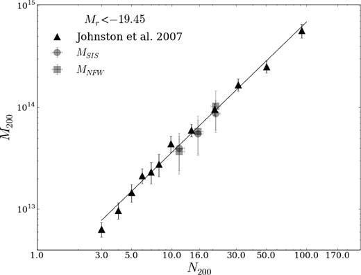
Mass–richness relation by Johnston et al. (2007) (solid line), together with M200 masses used to obtain that relation (triangles) and our mass estimates ( squares for NFW masses and circles for SIS masses) versus N200 from the maxBCG catalogue.
5.2 Yang group results
We determine the mean mass for four subsamples of the Yang group catalogue described in Section 3.3: Nmembers = 1, 2, 3 and 4 to 6. As it was done previously for the maxBCG sample, only groups in i-band frames with seeing values lower than 1.3 arcsec are analysed. The density profiles are shown in Fig. 3, and their best-fitting parameters are given in Table 2. NFW and SIS masses are in good agreement, |$\langle M^{{\rm NFW}}_{200}/M^{{\rm SIS}}_{200} \rangle = 0.91 \pm 0.03$|, showing that in contrast to massive clusters, an SIS profile is a suitable model to describe the mass distribution of low-mass systems.
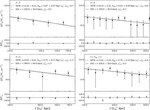
Same as Fig. 1, for the Yang sample.
Yang groups results.
| Selection criteria | NLens | 〈zLens〉 | S/N | SIS | NFW | |||
|---|---|---|---|---|---|---|---|---|
| σV | M200 | c200 | R200 | M200 | ||||
| (km s−1) | (|$10^{12} h_{70}^{-1} \,\mathrm{M}_{{\odot }}$|) | (|$h_{70}^{-1}$| Mpc) | (|$10^{12} h_{70}^{-1} \,\mathrm{M}_{{\odot }}$|) | |||||
| N = 1 | 7348 | 0.13 | 4.6 | 260 ± 30 | 15 ± 6 | 4.50 ± 0.22 | 0.47 ± 0.07 | 13 ± 5 |
| N = 2 | 4875 | 0.15 | 5.5 | 350 ± 40 | 35 ± 13 | 4.15 ± 0.21 | 0.63 ± 0.08 | 32 ± 13 |
| N = 3 | 1669 | 0.14 | 4.9 | 390 ± 60 | 52 ± 22 | 4.03 ± 0.21 | 0.73 ± 0.11 | 50 ± 22 |
| 4 ≤ N ≤ 6 | 1698 | 0.14 | 5.4 | 430 ± 50 | 71 ± 26 | 3.93 ± 0.19 | 0.79 ± 0.10 | 64 ± 25 |
Notes. Column (1): selection criteria to limit the sample of groups for stacking; column (2): number of groups considered in the stack; column (3): average z of the sample; column (4): S/N ratio as defined in equation 3; columns (5) and (6): results from the SIS profile fit, the velocity dispersion and |$M^{{\rm SIS}}_{200}$|; columns (7), (8) and (9): results from the NFW profile fit; c200 adopted according to |$M^{{\rm SIS}}_{200}$| and 〈zLens〉 (see text for details), and R200 and |$M^{{\rm NFW}}_{200}$|.
In Fig. 4, we plot the distribution of Mh obtained by Yang et al. (2012) for each subsample together with our lens mass determinations. For the four subsamples, we observe a good agreement between our lens masses and masses derived from mass-to-light ratios.
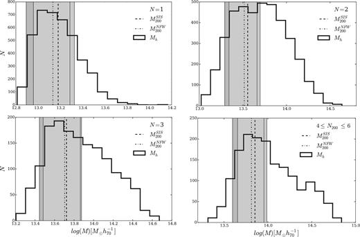
Distribution of halo masses computed by Yang et al. (2012) in the four richness bins, together with our lensing mass estimates (vertical lines and shaded regions for the corresponding errors).
We use these results to compare them with the P(M∣N) relation. As explained in Section 2, HOD cannot be directly compared with the lensing mass–richness relation so it is necessary to compute P(M∣N). We derive this distribution by using the same background subtraction method as in Rodriguez et al. (2015), computing average halo masses in richness bins. We consider only galaxy group members with Mr < −21.5. Hence, these distributions can be directly compared with the mass–richness relation obtained from this sample of groups. In Fig. 5, we plot P(M∣N) and M200 versus N. As it can be noticed that lens mass determinations by both models, SIS and NFW, agree with the P(M∣N) relation.
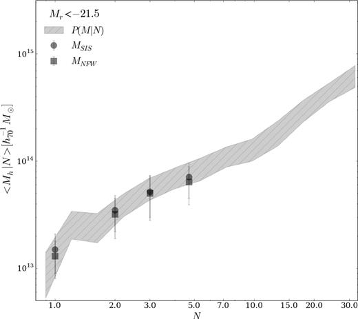
P(M∣N) obtained for SDSS DR7 implementing the background subtraction method for a limiting absolute magnitude |$M^{{\rm lim}}_{r} = -21.5$|. Squares and circles represent weak-lensing |$M^{{\rm NFW}}_{200}$| and |$M^{{\rm SIS}}_{200}$| masses versus N, respectively.
6 DISCUSSION AND CONCLUSIONS
In this work, we derive a mass–richness relation obtained by a weak-lensing analysis and compare it with P(M∣N) estimated through a straightforward background subtraction technique. To test our lens analysis, we estimated masses for a sample of maxBCG clusters by modelling the dark matter halo using both SIS and NFW model mass profiles. Our results are consistent with the mass–richness relation obtained by Johnston et al. (2007), who analysed an extended maxBCG sample with richness values N200 ≥ 3. We have also performed a weak-lensing analysis for a sample of low-richness groups from the catalogue of Yang et al. (2012) with results well described by NFW and SIS models.
Following the technique described by Rodriguez et al. (2015), we computed P(M∣N) from the same data set as used to estimate HOD restricted to a limiting absolute magnitude Mr = −21.5. This distribution is compared with the mass–richness relation obtained for the Yang group sample in Fig. 5, where it can be seen a good agreement between both relations. In particular, we stress the fact that our result for Nmember = 1 is consistent with P(M∣N). These groups include systems that are composed of only one galaxy with redshift information available, making it impossible to estimate their virial masses. However, our stacking lensing analysis allows us to derive the average system mass.
The agreement between the M–N relation and P(M∣N) reinforces the confidence in the method employed in computing HOD based on background subtraction techniques. Besides, it presents a new approach to test the mass–richness relation. It is important to highlight that these results cannot be directly compared with other HOD analysis (e.g. Tinker et al. 2012; Guo et al. 2015) since we adopt richness instead of mass bins. In our analysis, we used the same information as in the computation of HOD to obtain P(M∣N) in a straightforward way, allowing for a direct comparison between two independent relations, lensing mass–richness and P(M∣N). This result can be extended to fainter limiting magnitudes, which could provide a deeper understanding of the relation between galaxies and mass distribution in haloes.
Acknowledgments
We thank Miriam Zorn for her careful reading and corrections to the manuscript. We also thank the anonymous referee for their very useful comments that improved the content and clarity of the manuscript. This work was partially supported by the Consejo Nacional de Investigaciones Científicas y Técnicas (CONICET, Argentina) and the Secretaría de Ciencia y Tecnología de la Universidad Nacional de Córdoba (SeCyT-UNC, Argentina).
We made an extensive use of the following python libraries: http://www.numpy.org/, http://www.scipy.org/, http://roban.github.com/CosmoloPy/ and http://www.matplotlib.org/.
