


Abstract
Motivated by the non-linear star formation efficiency found in recent numerical simulations by a number of workers, we perform high-resolution adaptive mesh refinement simulations of star formation in self-gravitating turbulently driven gas. As we follow the collapse of this gas, we find that the character of the flow changes at two radii, the disc radius rd and the radius r*, where the enclosed gas mass exceeds the stellar mass. Accretion starts at large scales and works inwards. In line with recent analytical work, we find that the density evolves to a fixed attractor, ρ(r, t) → ρ(r), for rd < r < r*; mass flows through this structure on to a sporadically gravitationally unstable disc and from thence on to the star. In the bulk of the simulation box, we find that the random motions vT ∼ rp with p ∼ 0.5 are in agreement with Larson's size–linewidth relation. In the vicinity of massive star-forming regions, we find p ∼ 0.2–0.3, as seen in observations. For r < r*, vT increases inwards, with p = −1/2. Finally, we find that the total stellar mass M*(t) ∼ t2 is in line with previous numerical and analytic work that suggests a non-linear rate of star formation.
1 INTRODUCTION
Whether this low efficiency applies to scales comparable to giant molecular clouds (GMCs), with radii of the order of 100 pc, is debated in the literature. Heiderman et al. (2010), Lada, Lombardi & Alves (2010), Wu et al. (2010), and Murray (2011) find efficiencies ε ∼ 0.1 − 0.5, while Krumholz & Tan (2007) and Krumholz, Dekel & McKee (2012a) find ε ≈ 0.01. On these small scales, observations also suggest that the efficiency is not universal, but instead varies over two to three orders of magnitude (e.g. Mooney & Solomon 1988; Lee, Miville-Deschenes & Murray 2016).
There are a number of explanations for the low star formation rate, on either small or large scales (although they may not be necessary for the former). These include turbulent pressure support (Myers & Fuller 1992), support from magnetic fields (Strittmatter 1966; Mouschovias 1976), and stellar feedback (e.g. Dekel & Silk 1986). Numerical experiments investigating the first two effects suggest that neither turbulence nor magnetic support is sufficient to reduce the rate of star formation to ε ≈ 0.02 on small scales (Wang et al. 2010; Cho & Kim 2011; Padoan & Nordlund 2011; Krumholz, Klein & McKee 2012b; Myers et al. 2014). Feedback from radiative effects and protostellar jets and winds may be able to explain the low star formation rate, but the impact of these forms of stellar feedback remains uncertain despite recent progress (Wang et al. 2010; Myers et al. 2014; Federrath 2015).
Until very recently, galaxy-scale or larger (cosmological) simulations were not able to reproduce the Kennicutt–Schmidt relation. Nor did the cosmological runs reproduce correctly the mass of stars in galaxies of a given halo mass, despite including supernova and other forms of feedback, e.g. Guo et al. (2010), Governato et al. (2010), and Piontek & Steinmetz (2011). To overcome this low resolution-driven problem, Hopkins, Quataert & Murray (2011, 2012) performed high-resolution (few parsec spatial, few hundred solar mass particle masses) simulations of isolated galaxies, modelling both radiative and supernovae feedback (among other forms). They recovered the Kennicutt–Schmidt relation, a result that they showed was independent of the small-scale star formation law that they employed. The simulations in the second paper also generated galaxy-scale outflows or winds, removing gas from the disc, thus making it unavailable for star formation. When the feedback was turned off, the star formation rate soared, demonstrating that in the simulations, at least, feedback was crucial to explaining the Kennicutt–Schmidt relation and the outflows. Simulations including supernovae but lacking the radiative component of the feedback did not exhibit strong winds and so overproduced stars.
Cosmological simulations employing unresolved (or ‘sub-grid’) models for both radiative and supernovae feedback are now able to reproduce the halo–mass/stellar mass relation (e.g. Aumer et al. 2013; Hopkins et al. 2014; Agertz & Kravtsov 2015). Again, these simulations require stellar feedback to drive the winds that remove gas from the disc, so as to leave the observed mass of stars behind.
Lee, Chang & Murray (2015) emphasized that the star formation efficiency (SFE) on parsec scales is non-linear in time, i.e. ε∝t which implies M*∝t2 on small scales, where M* is the total stellar mass. Magnetic fields slowed the initial star formation rate somewhat, but did not change the M*(t) ∼ t2 scaling. Using a detailed numerical simulation, they showed that this non-linear star formation rate is driven by the properties of collapsing regions. In particular, they demonstrated that the turbulent velocity near or in collapsing regions follows different scaling relations than does turbulence in the global environment which follows Larson's law, vT(r) ∼ r1/2 (Larson 1981). They also showed that the density PDF is not lognormal, but rather develops a power law to high density. This latter result was hinted at by Klessen (2000) and shown convincingly as well as explained by Kritsuk, Norman & Wagner (2011).
The increasing rate of star formation found by Lee et al. (2015) is important in that it may provide an explanation for the observed range in star formation rates on small scales. It suggests that the star formation rates on small scales vary in part because of the age of the star-forming region; slow star-forming regions, with very low instantaneous efficiencies, will ramp up their stellar production over time. If this result can be firmly established, it will highlight the need for a form of very rapid feedback. In particular, since the dynamical time in massive star-forming regions is much smaller than the time delay of ∼ 4 Myr between the start of star formation and the first supernovae, rapid star formation on small scales would have to be halted by some form of feedback other than supernovae.
The simulations of Lee et al. (2015) explicate the link between the rate of star formation with the gravitational collapse of high-density regions, which is an analytically well-studied problem. An early model of Shu (1977) estimated the accretion rate on to stars by assuming that stars form from hydrostatic cores supported by thermal gas pressure. The accretion rate in his model was independent of time, given by |$\dot{M} = m_0c_{\rm s}^3/G$|, where cs = (kbT/μ)1/2 is the sound speed in molecular gas and m0 = 0.975. Shu (1977) predicted a maximum accretion rate of |${\sim } 2\times 10^{-6} \,\text{M}_{\odot }\,\,\rm yr^{-1}$|, which is too small to explain the origin of massive (|$M_{\ast }\sim 50\text{--}100\,\text{M}_{\odot }$|) O stars, which have lifetimes ≲ 4 × 10⁶ yr.
Myers & Fuller (1992) overcame the difficulty with slow accretion rates by adopting the turbulent speed in lieu of the sound speed (see also McLaughlin & Pudritz 1997 and McKee & Tan 2003). In doing so, they were able to replace the slower signal speed of sound with the faster turbulent speed. However, they continued to assume that the initial condition was that of a hydrostatic core which is supported by turbulent pressure. They also assumed that the turbulence is static and unaffected by the collapse.
Collectively, these models (Shu 1977; Myers & Fuller 1992; McLaughlin & Pudritz 1997; McKee & Tan 2003) are referred to as inside-out collapse models; the collapse starts at small radii (formally at r = 0 in the analytic models) and works its way outwards, at the assumed propagation speed (cs or vT(r)). At any given time, the infall velocity and mass accretion rate both decrease with increasing radius r. The analytic models assume the existence of a self-similarity variable x = r/vt, where v = cs in Shu (1977) or the turbulent velocity vT(r) in Myers & Fuller (1992), McLaughlin & Pudritz (1997), and McKee & Tan (2003). These models predict velocity and mass accretion profiles very different than those seen in the simulations of Lee et al. (2015).
MC15 used this in place of an energy equation. Together with the equations for mass continuity and momentum, equation (2) gives a closed set of equations that can be solved in spherical symmetry numerically. In addition, they were able to analytically show that the results of their calculations gave density and velocity profiles that appear to be in line with both recent numerical calculations (Lee et al. 2015) and observations (e.g. Caselli & Myers 1995; Plume et al. 1997).
To summarize, MC15's major results were as follows.
The gravity of the newly formed star introduces a physical scale into the problem which MC15 called the stellar sphere of influence, r*. This is an idea familiar from galactic dynamics. The radius r* is where the local dynamics transitions from being dominated by the mass of the gas to being dominated by the mass of the star. As a result, the character of the solution, in particular that of the velocity, differs dramatically between r < r* and r > r*. The existence of this physical scale modifies the form of the self-similarity on which inside-out theories rely.
- The small-scale density profile is an attractor solution. MC15 showed numerically and argued analytically that at small scales, the density profile is an attractor solution. In particular, MC15 showed the density profile asymptotes to:where r0 is some fiducial radius.(3)\begin{eqnarray} \rho (r,t)&=& \Bigg\{\begin{array}{l@{\quad}l} \rho (r_0)\left({\frac{r}{r_0}}\right)^{-3/2},& r<r_{\ast }(t)\\ \rho (r_0,t)\left({\frac{r}{r_0}}\right)^{-k_{\rho} },\quad \ k_{\rho} \approx 1.6\!-\! 1.8 & r>r_{\ast }(t) \end{array},\nonumber\\ \end{eqnarray}
- The existence of r* implies that the infall and turbulent velocities have different scaling for r < r* and r > r*. In particular, MC15 showedThus, the scaling of the turbulent velocity differs from that predicted by Larson's law (∝ r1/2) inside the sphere of influence. In other words, the turbulent velocity in massive star-forming regions will deviate from Larson's law, which has long been observed, but without theoretical explanation.(4)\begin{equation} u_{\rm r}(r,t), v_{\rm T}(r,t) \propto \left\{\begin{array}{l@{\quad}l} \sqrt{\frac{GM_{\ast }(t)}{r}} \sim r^{-1/2} & r<r_{\ast }(t)\\ \sqrt{\frac{GM(r,t)}{r}} \sim r^{0.2} & r>r_{\ast }(t) \end{array}. \right. \end{equation}
The stellar mass increases quadratically with time. This result arises naturally from the attractor solution nature of the density profile at small r, equation (3), and the scaling with Keplerian velocity for the turbulent and infall velocities at small r, equation (4).
The mass accretion rate:(5)\begin{equation} \dot{M}(r,t)= \left\{\begin{array}{l@{\quad}l} 4\pi R^2\rho (R)u_{\rm r}(r,t), \sim t\,r^{0} & r<r_{\ast }\\ 4\pi R^2\rho (R)u_{\rm r}(r,t) \sim t^0\,r^{0.2} & r>r_{\ast }. \end{array} \right. \end{equation}
MC15's predictions for r < r* could not be checked using the simulations of Lee et al. (2015) as those fixed grid simulations were too coarse. In this paper, we study the collapse of gas and formation of stars in a turbulent GMC using roughly a dozen high-resolution adaptive mesh refinement (AMR) simulations in this paper.
We employ large-scale (16 pc) hydrodynamic AMR simulations of star-forming clouds with continuously driven supersonic turbulence. The initial conditions for our simulations are exactly the same as the flash simulations in Lee et al. (2015).
If the equations are non-dimensionalized, two dimensionless variables appear, the Mach number |${\cal M}$| and the virial parameter |$\alpha _{\text{vir}} \equiv (5/3) v_{\rm T}^2 / GM_{\text{box}}$|, e.g. Mihalas & Mihalas (1984). We want to model massive star-forming regions in the Milky Way, so we choose the Mach Number |${\cal M} = 9$| and the virial parameter αvir = 1.9, respectively. In addition, we choose the size of the box L = 16 pc and the sound speed cs = 0.264 km s−1, so that the turbulent velocity lies approximately on the observed size–linewidth relation, Larson's law. These choices fix both the density and the mass scale.
The simulations described in this paper disregard several physical effects. We do not include radiative, stellar wind, or protostellar jet feedback. While the feedback physics we neglect can have significant effects on both the rate of star formation and the initial mass function (IMF), we aim to address the role the random motions captured by the Reynolds stress play in the dynamics of gravitational collapse in turbulent fluids.
Our equation of state is that of an isothermal gas. It is possible, and even likely, that thermal effects play a role in setting the IMF of stars, e.g. Larson (2005). With this in mind, we relegate the discussion of the IMF to an appendix, as the details are unlikely to be reliable.
This paper is organized as follows. In Section 2, we describe our numerical methods and simulation setup. In Section 3, we present and analyse the results of our simulations. In particular, we make detailed comparisons with the results of MC15. We discuss our results and compare them to previous work in Section 4
2 DETAILED SIMULATIONS OF TURBULENT COLLAPSE
Most of the simulations described here use the AMR code flash version 4.0.1 (Fryxell et al. 2000; Dubey et al. 2008) to model self-gravitating, hydrodynamic turbulence in isothermal gas with 3D periodic grids and a minimum of eight levels of refinement on a root grid of 1283, giving an effective resolution of 32 7683. Following Lee et al. (2015), our flash runs use the Harten-Lax-van Leer-Contact Riemann solver and an unsplit solver (Lee, Deane & Federrath 2009). We have also used the ramses code (Teyssier 2002), but unless explicitly stated otherwise, the results below come from flash simulations.
As just mentioned, we start with a box with the physical length set to L = 16 pc using periodic boundary conditions. The initial mass density is ρ = 3 × 10⁻²² g cm−3 (number density n ≈ 100 cm−3), corresponding to a mean free-fall time |$\bar{\tau }_{\rm ff}\approx 3.8\,{\rm Myr}$|; the total mass in the box is M ≈ 18 000 M⊙. The sound speed is set to cs = 0.264 km s−1. We use pure molecular hydrogen in this simulation so the ambient temperature T ≈ 17 K.
To initialize our simulations, we drive turbulence by applying a large-scale (1 ≤ kL ≤ 2, corresponding to 1.3–2.7 pc) fixed solenoidal acceleration field as a momentum source term. We use solenoidal driving because it is known that compressive turbulence increases the star formation rate compared to solenoidal driving (Federrath, Klessen & Schmidt 2008). We apply this field in the absence of gravity and star particle formation for three dynamical times until a statistical steady state is reached. The resulting Mach number is |${\cal M} = 9$|, i.e. a turbulent velocity of vT = 2.37 km s−1.
Stirring the initial turbulence using a fixed driving field is a technique used by a number of workers in the field (Collins et al. 2011; Padoan & Nordlund 2011). Other groups initialize the turbulence by initializing the velocity field with Gaussian random perturbations having some assumed power spectrum (Myers et al. 2014; Skinner & Ostriker 2015). While neither of the resulting velocity fields are generated the way the turbulence in the interstellar medium (ISM) of our Galaxy is, the stirring allows one to perform simulations which have non-trivial initial density structures and velocity fields that are at least reminiscent of those inferred from observations of the ISM of our Galaxy.
Federrath & Klessen (2012) use a time-varying driving field to produce random motions. They argue that a time-varying driving field allows one to avoid large spatial correlations which would result from a fixed driving field acting for a time longer than the dynamical time of the simulation box. In our simulations, we do not run for longer than a box dynamical time after turning on star formation. We run for 600 000 yr, about 0.16 dynamical times, after the first star forms. The limiting factor on the length of the runs was our available compute time. Hence, we do not expect the large-scale turbulent flow to vary much over such a short time. In addition, there is some evidence (Federrath et al. 2010a) that the results of turbulent driving are not sensitive to the exact large-scale mechanism.
This fully developed turbulent state is the initial condition to which we add self-gravity and star particle formation for our star formation experiments. We enable AMR to follow the collapse of overdense regions. Even after turning on star formation, we continue to drive the large-scale fixed solenoidal acceleration field.
In the appendix, we describe a number of test simulations in which we refined the grid when NJ = 4, 8, 16, or 32 (Federrath et al. 2011). We show that many of the quantities in our runs, including the density and the mass accretion rates, are converged for NJ = 4.
The maximum dynamic range is a little larger than six orders of magnitude because we allow the density to increase further before forming star particles. When the Truelove criterion is exceeded by a factor of 3 at the highest refinement level, the excess mass in a cell is transferred either to a newly created star particle or to a star particle whose accretion radius includes the cell. The factor of 3 allows only the highest density regions to form star particles. It is inspired by the work of Padoan & Nordlund (2011) whose sink particle formation criteria of 8000× mean density is a factor of 3 to 4 above the Truelove criteria at their highest resolution of 10003. Additionally, the three cells immediately around a star particle can rise above this density criterion. This is done so that we do not form star particles within two cells of each other. Instead, these close surrounding cells can only accrete on to the previously formed star particle. We should also note that like our previous work in Lee et al. (2015), our star particle creation prescription is different from the prescription of Federrath et al. (2010b) where additional checks are performed; in the appendix, we present the results of runs in which we used these additional checks, finding that they do not affect the t2 scaling of the stellar mass, or the dynamics of the infall.
To calculate the gravity, we use the same algorithm as described in Lee et al. (2015) which we now briefly describe. To compute the self-gravity on the gas, we first map star particles to the grid and then use a multigrid Poisson solver (see Ricker 2008), coupled with a fast-Fourier transform (FFT) solution on the root grid, to solve for gravity. To compute the gravitational acceleration on the star particles, we first compute the particle–particle forces using a direct N-body calculation. To compute the particle–gas forces, we use the same multigrid solver (with root grid FFT) on the grid, but with the star particle unmapped. As a result, two large-scale gravity solutions (one with and one without mapped star particles) must be found per timestep as opposed to one. This allows us to avoid the computationally expensive task of computing gas–star particle forces via direct summation. As discussed in Lee et al. (2015), this splitting of particle-particle and particle–gas/gas–particle forces does not strictly obey Newton's second law, breaking down at roughly the size of the smallest grid cell. As a result, errors in the orbits of particles may result. However, we believe that our runs are short enough to avoid the buildup of significant errors.
In the flash runs, to obtain a useful number of star particles with long accretion histories, we have taken the initial turbulent box and have only run our refinement algorithm (and hence, star particle algorithm) on only one octant at a time. This forces us to run eight high-resolution simulations, each on a difference octant and so allows us to treat each octant as a separate distinct simulation. This is necessary as flash does not have individual timesteps, which results in the code grinding to a halt once a single region collapses.
3 RESULTS
In Fig. 1, we show a projection along the z-axis of the entire simulation volume for one of the high-resolution octant simulations, 2.8 Myr after gravity has been turned on. The image shows up to eight levels of refinement, giving an effective resolution of 32 7683 or a minimum cell size of 5 × 10− 4 pc. Regions that are highly refined are the densest regions, for which the image is smoother than the low-density more pixelated regions. Note that the highly refined regions are limited to the lower right which is the octant that this particular simulation focused on. The other seven simulations refine the other octants.
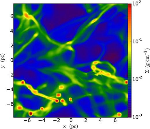
Projection of the density along the z-axis of the entire simulation volume. The root grid is 1283 with up to eight levels of refinement, giving an effective resolution of 32 K3. This snapshot is taken 2.8 Myr after star formation was turned on.
The high-density regions are organized into filaments. These filaments span most of the simulation box, with lengths up to several parsecs and widths of the order of a few tenths of a parsec. Some filaments appear to flow into large clumps. This is in accord with many previous simulations, e.g. Padoan et al. (1998) and Lee et al. (2015). These clumpy regions have the highest densities and hence are the first to fulfill the criterion for star particle formation.
In this section, we focus on the regions around two individual star particles which we refer to as particle A and particle B.
Particle A formed about a quarter of a parsec away from its nearest neighbour star particle. At the end of the run, it was ∼736 000 yr old and had a mass of ∼17.5 M⊙, although it was still accreting rapidly.
Particle B formed and remained in isolation. At the end of the run, the particle was ∼512 000 yr old and had a mass of ∼10.7 M⊙. Throughout the simulation, particle B had a steady supply of gas.
3.1 The run of infall (|$\boldsymbol {v}_{\rm r}$|), circular (|$\boldsymbol {v}_\phi$|), and random motion (|$\boldsymbol {v}_{\rm T}$|) velocities with radius (r) before star particle formation
Fig. 2 shows the infall velocity (ur), circular (vϕ), and random motion (vT) velocities as a function of radius (top panel) and the density in a slice of the local volume (bottom panel) around the density peak that will form particle A in 100 000 yr in the future. In Appendix A, we describe how we calculate each of these velocities.
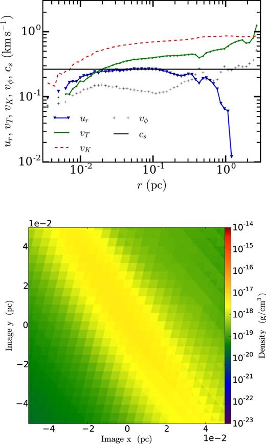
The top plot shows the run of velocity with radius measured from the density peak; this density peak will develop into particle A in 100 000 yr. The sound speed is the black horizontal line, while the infall velocity |ur| is given by the blue triangles, connected by a solid blue line. The green circles connected by a solid green line show vT, while the black crosses show the rotational velocity vϕ. The red dashed line is the Keplerian velocity |$v_{\rm K}\equiv \sqrt{GM(r)/r}$|. Even at this early stage, the structure is far from hydrostatic equilibrium, as the infall velocity is ∼25 per cent of the free-fall velocity. The refinement level is l = 6, which corresponds to a cell size of ∼ 2 × 10− 3 pc. The bottom plot shows the density in a slice along the direction of the angular momentum vector centred on that peak.
We will compare vT to what MC15 referred to as a turbulent velocity. Our current definition of vT is simply that of a random velocity. We are agnostic about whether or not vT characterizes an isotropic turbulent pressure; close examination of the velocity field indicates that the random motions are not isotropic on the scale of their distance from the density peak. It is also clear, however, that vT characterizes a Reynolds stress that does provide a net outward support against gravitational collapse. This follows from a simple energy argument; the infall velocity in the vicinity of the density peak is well below the local free-fall velocity and remains so throughout the simulation, even after a star particle forms. Thus, some of the potential energy released by the infall goes into some channel other than inward motion. A fraction of the potential energy release goes into shocks and, in our code, is effectively removed immediately. At this early stage, the rotational motion represents a small fraction (≲ 10 per cent) of the energy at all but the smallest radii. But the inward flattening of the green line in Fig. 2 and the inward increase seen in later figures show that a substantial fraction of the potential energy released by the inflow goes into random motions. By energy conservation, this fraction is not available to the inflow, so that |ur| is smaller than it would be if the random motions were not absorbing some of the energy. This shows that there is an effective outward force on the infalling gas.
The infall velocity, ur, and random motion (vT) velocity are similar in magnitude, and somewhat smaller than the Keplerian velocity, |$v_{\rm K} = \sqrt{GM(<r) /r}$|. Note that ur is roughly equal to the sound speed while vT is supersonic. The fact that the infall velocity is ∼25 per cent of the free-fall velocity over all radii less than a parsec shows that this system is not in hydrostatic equilibrium. The density distribution is smooth and filamentary. The run of density versus radius, which is not shown, is a simple power law with a small inner core.
Fig. 3 shows the region around the same density maximum some 70 000 yr later, 30 000 yr before star particle A forms. Once again the infall velocity is a substantial fraction of the Keplerian velocity, showing that the core remains far from hydrostatic equilibrium. However, vϕ in the innermost regions (inside 0.01 pc) is comparable to both vK and vT, showing that the innermost region is partially rotationally supported. The density slice shown in the bottom panel of Fig. 3 confirms this interpretation, showing a disc-like structure with a radius of the order of ∼ 0.01 pc. The mass inside this radius is ∼0.7 M⊙. We note that the particle forms near the tip of a filament (not shown).

The top panel shows the run of velocity around the same density peak as that shown in Fig. 2, but now only ∼30 000 yr before the formation of particle A. The colour and linestyles are the same as in the top panel of Fig. 2. The bottom panel again shows the density in a slice centred on the density peak. The plotted arrows show the velocity in the plane of the slice. The longest arrows correspond to roughly 2 km s−1. In the intervening ∼70 000 yr since the time shown in Fig. 2, an accretion disc-like structure has formed which has a mass of ∼0.7 M⊙. The radius of the sphere of influence (of the disc) is ∼0.02 pc. All three velocities, |ur|, vT, and vϕ, increase inwards of r*; the inflow is disrupted at r ∼ 0.015 pc: a feature that we interpret as a shock, where the flow meets the nascent accretion disc, at which point vT also drops in magnitude. At yet smaller radii, the infall resumes, because at this early time, the disc is not yet fully rotationally supported. The resolution at the location of the star particle has reached the refinement limit Δx = 5 × 10− 4 pc; the errors in the calculation of the velocities that are associated with the finite resolution are substantial inside r ≈ 0.002 pc, so features inside this radius are not reliable and thus not plotted.
3.2 The stellar sphere of influence
Equations (3), (4), and (9) predict that the character of the solution should change at r* and r* increases with time. Our numerical results support this prediction. Fig. 4 shows that vT decreases with decreasing radius down to r* and then increases with decreasing radius inside the sphere of influence. We see that vT reaches a minimum near r = r*. The inward decrease in vT(r) is not monotonic near 0.2 pc, probably due to a shock, as suggested by jumps in both the infall and random velocities and in the density at r ∼ 0.02 pc. This trend of increasing vT with decreasing radius inside r* is repeated in Fig. 5.
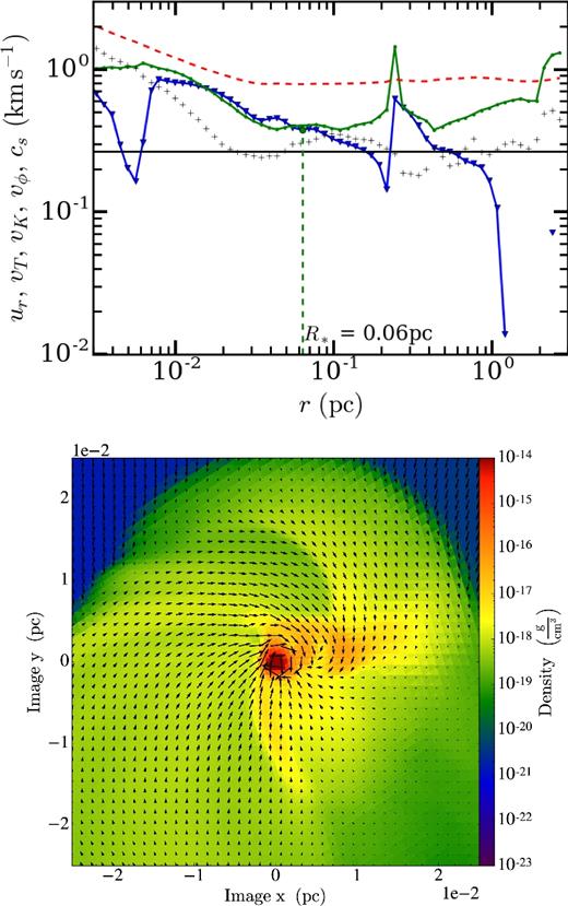
The run of velocity (top panel) of particle A 24 000 yr after star particle formation. The colour and linestyles are the same as in the top panel of Fig. 2. This panel shows that the disc around the particle is rotationally supported for r ≲ 5 × 10− 3 pc; inside that radius, the black pluses are higher than either the green or blue points, i.e. the rotational velocity is larger than either the random motion or infall velocity. The radius of the sphere of influence is r* ∼ 0.06 pc. The star mass is 2.47 M⊙ and the disc mass is 0.58 M⊙; thus, the disc is about 23 per cent the mass of the star. The bottom panel is a density slice centred on particle A, in the centre of mass frame, face-on to the rotationally supported disc. The arrows show the velocity in the plane of the slice. The longest arrows correspond to nearly 3 km s−1. With a cell size of Δx = 5 × 10− 4 pc, we have ∼20 cells across the diameter of the disc.
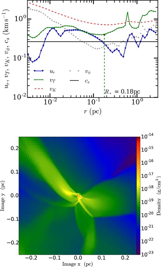
The top panel shows the run of velocity for particle B ∼100 000 yr after formation. The radius of the sphere of influence is 0.18 pc. The stellar mass is 4.5 M⊙ and the disc mass is 2.47 M⊙ so the disc is ∼55 per cent of the stellar mass. The bottom panel shows the density in a slice centred on particle B.
We do not see an increase in the infall velocity for r > r* for this object because the star particles are forming about 1 pc from the end of a filament, but we do see an increase in |ur| in other particles.
Comparing Fig. 4, which shows the velocity and density of the same region 24 000 yr after star particle A forms, with Fig. 3 demonstrates that the radius of the change in character of the flow associated with r* increases over time. In particular, the global minimum of the random motion velocity is now at 0.06 pc rather than somewhere between |$0.01\text{ and }0.02 \,\rm pc$|.
The drop in ur at large radii in Fig. 4 reflects the vagaries of the large-scale Reynolds stress pressure gradient; we already mentioned that this particle is forming near the end of a filament.
Fig. 5 shows the velocities and the density in a slice centred on particle B, 100 000 years after that star particle forms. This star is more isolated than particle A and as a result, |ur| increases from r ≳ r* out beyond r ≈ 3 pc. This is in accord with equations (4) and (5), but it contrasts with the result in Fig. 4.
The behaviour of |ur(r)| at large radii is not set by the collapse dynamics, but rather by the properties of the random motions, most importantly the outer scale of the Reynolds stress gradient. In particular, we do not expect |ur(r)| to be significant on scales larger than some moderate fraction, say one-fourth, of the outer scale. In our simulations, the outer scale is given by k = 2 or L/2 and we use solenoidal stirring so that the cascade starts out with no compressive component, although one develops as the cascade proceeds. In fact, we will show in Section 3.7 that the typical radius of a converging region is more like r ≈ 1 pc in our simulations.
3.3 A fixed point attractor for ρ(r, t) inside r*
One of the most striking findings of MC15 was that the run of density is independent of time for r < r*. Our simulations confirm that finding, as illustrated in Fig. 6. The plot shows the run of density for two separate times. The dotted blue line shows the run of density ∼40 000 yr before particle A forms, while the solid green line is the run of density ∼540 000 yr after the star particle forms. The elapsed time corresponds to nearly two-tenths of the mean free-fall time of the box and to many free-fall times at radii less than a tenth of a parsec. We emphasize that the density can change on the local free-fall time, which is much smaller than the global free-fall time (by a factor of 10 or more for r < 0.1 pc). We will show that in fact the density inside rd does change rather rapidly, after the star particle forms, but that for rd < r < r*, the density does not change; see Section 3.7.
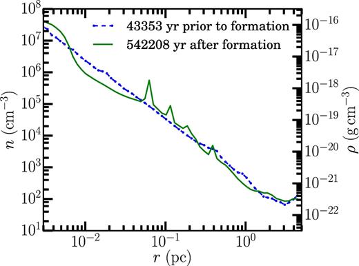
The run of density for particle A. The dotted blue line is the density ∼40 000 yr before the star forms. The solid green line is the run of density ≈540 000 yr after formation. The gap in time corresponds to the free-fall time at a radius of 0.24 pc. For r < 0.24 pc, the range of time spanned in the plot is more than a local free-fall time, yet the density does not vary significantly. There are fluctuations in the density, e.g. the spikes around r ∼ 0.1 pc. In Fig. 9, we average over a number of objects to remove these fluctuations: we also demonstrate that the density in the disc does increase.
The mean power-law slope of the density before the star forms (the blue dashed line in the figure) is kρ ≈ 1.9, consistent within the star-to-star variations we see with the range kρ ≈ 1.6–1.8 from equation (3) for r > r* (since in this case, r* = 0).
3.4 Mass accretion rate
In Fig. 7, we show the mass accretion rate |$\dot{M}$| as a function of r around a star particle (t − t* > 0) and from the corresponding density peak in which the star particle eventually formed (t − t* < 0). This plot is taken from a ramses simulation. Before the star particle forms, |$\dot{M}$| decreases inwards at all radii.
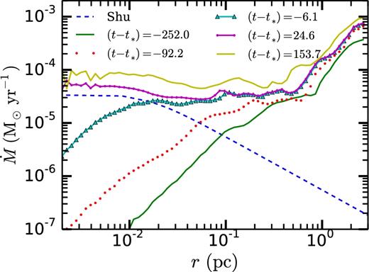
The run of |$\dot{M}$| for a star particle in a simulation with NJ = 32 cells per Jeans length resolution, at a maximum effective resolution of 16 3843. The lowest solid (green) line is the run of |$\dot{M}$| for the density peak which will form the star particle 252 000 yr after the time plotted. The accretion rate is about an order of magnitude lower at small radii (say 10− 2 pc) than at 1 pc. The purple line connecting the dots is the run of accretion soon after the star particle forms, when the stellar mass is about a solar mass. The accretion rate at 1 pc still exceeds that at all smaller radii, showing that the collapse is outside-in, not inside-out. As an example of an inside-out collapse, we show the accretion rate for the Shu (1977) model (the dashed line) for a star of a solar mass with A = 5.5.
Following the establishment of the power-law solution for the density, at t = t*, a star particle forms and the |$\dot{M}$| profiles flatten at small radii. An examination of the density profile (not plotted) reveals that ρ ∝ r−3/2, while for t − t* = 24 kyr, the gravitational force (and hence ur) is dominated by the central mass for r ≲ 0.1 pc, so that v ∝ r−1/2 out to that radius. We also note that while the |$\dot{M}$| profile is flat, it does increase in time as shown by the difference between the t − t* = 24.6 and 154 kyr curves. All this behaviour agrees well with the prediction of equation (5).
At all times, the accretion rate is either nearly flat or increasing with radius, which is a natural result of the near balance between gravity and Reynold's stress support, as posited in the theory of MC15. We contrast this with an inside-out collapse model which we exemplify using a Shu (1977) solution (blue dashed line) obtained by directly integrating equations (11) and (12) of Shu (1977) at a fixed time. The asymptotic behaviour of |$\dot{M}$| follows from Shu's equations (15) and (17); recall that x = r/(cst) is a function of the radius. In the limit of small x, |$\dot{M}$| approaches a constant. However, for large values of x, |$\dot{M}(r,t)=-A(A-2) c_{\rm s}^3/Gx$| (equation 15 of Shu 1977), i.e. the mass accretion rate falls like 1/r at a fixed time at large r as seen in Fig. 7.
In other words, for inside-out collapse models, the accretion rate is monotonically decreasing with increasing radius. This is qualitatively different from the prediction of MC15 or the results of this work. We note that while we have chosen to plot the Shu solution, other collapse solutions (McLaughlin & Pudritz 1997; McKee & Tan 2002, 2003) have the same general profile: the mass accretion rate is roughly independent of r at small radii and decreases with increasing r at large radii.
In summary, at no time do we see any indication of an inside-out collapse in our simulated massive star-forming regions.
3.5 Rotationally supported discs
Many of the qualitative and even quantitative features predicted by MC15 are found in our simulations as discussed above, including the approach of the density profile inside r* to an attractor solution, the minimum in the velocity profile around the sphere of influence, and the expansion of the sphere of influence with time. However, our simulations display additional dynamics that were not modelled by MC15.
A particularly interesting bit of dynamics neglected by MC15 is the development of a rotationally supported disc which we alluded to above. This development is evident in the velocity plots, starting from the absence of a disc in Fig. 2 to a protodisc with no central star particle in Fig. 3 to a fairly well-developed rotationally dominated disc, at r ≲ 0.05 pc in Fig. 4.
We define the outer edge of the accretion disc rd as the largest radius where vϕ exceeds both |ur| and vT, i.e. where the disc is rotationally dominated. The development of the disc is best followed by examining the rotational velocity seen in Figs 2–4. In the last figure, rd ≈ 7 × 10− 3 pc. We have also used a second definition for the disc radius, i.e. where the derivative of the density has a sharp drop; see footnote 1. The two definitions of the disc radii agree well with each other.
We note that the discs in our simulation have rd ∼ 1000 au. This is somewhat larger than the radii of the largest observed discs, e.g. Padgett et al. (1999) find 500 au ≲ rd ≲ 1000 au. Of course we are simulating massive star formation and most observations of discs are of nearby, low-mass stars. Another factor to keep in mind is that we are doing hydrodynamic simulations, so there are no magnetic fields which are believed to be effective at transporting angular momentum; the inclusion of magnetic fields might therefore tend to reduce the sizes of the accretion discs in our simulations.
3.6 Gravitationally unstable discs
The plot of |$\dot{M}$| in Fig. 7 shows that the accretion rate varies little across the transition from the rotationally supported disc to the radial infall-dominated part of the flow at slightly larger radii. In other words, the disc is transporting angular momentum efficiently enough so that the disc accretion rate matches the rate at larger radii. Since our simulations do not include magnetic fields, this efficient disc accretion is not due to the magneto-rotational instability (Balbus & Hawley 1991, 1998).
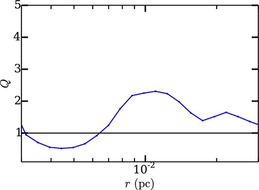
The Toomre Q parameter for particle B , at the same time as shown in Fig. 5, ∼100 000 yr after star particle formation. From Fig. 5, we see that the disc is rotationally dominated for r < 2 × 10− 2 pc. For 3 × 10− 3 ≲ r ≲ 6 × 10− 3 pc, Q ≲ 1. This indicates that the disc is gravitationally unstable at these radii, while it is marginally stable at larger radii. Fig. 14 provides a more representative view of disc stability.
3.7 Average profiles
Thus far, we have focused our attention on two of our stars and shown that their vT, ur, and ρ profiles are qualitatively similar to the profiles predicted in the analytic work of MC15. Now we will show that this behaviour is generic in the sense that this is true, on average, over all the star particles in our simulations. At the end of our base flash simulations, we have found roughly 60 star particles. To study these systems in a generic way, we look at the average velocity and density profiles. Motivated by the results of MC15, we average the profiles at fixed stellar mass; by fixing the stellar mass, we fix r* and hence the velocity, ρ, and |$\dot{M}$| profiles.
For epochs before a star particle forms, it is less clear how these profiles should be averaged. However, equation (3) predicts that ρ(r, t) approaches a time-independent function as soon as any non-pressure supported structure, such as a disc, forms. As a result, we elect to follow the methodology in Lee et al. (2015) and average profiles at fixed times (10 and 100 kyr) before the formation of a star particle. The choice of these two times allows us to study the conditions in the collapsing region immediately before and well before the formation of the star particle, while retaining several (six to seven) density peaks and hence reasonable statistics.
In Fig. 9, we plot n as a function of r, 10 000, and 100 000 yr before star particle formation (left-hand plot) and for stellar mass M* = 1 and 4 M⊙ (right-hand plot). The plots show that ρ(r, t) → ρ(r) for rd < r < r*, i.e. the density approaches the attractor solution, early in the collapse, and this profile persists through formation of the star particle and well after. This generalizes what we found for our two example star particles in Section 3.3.
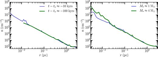
Number density as a function of radius at 10 000 and 100 000 yr before the star particle forms (left-hand plot) and when the star reaches 1 and 4 M⊙ (right-hand plot). For the left-hand plot, we average over six and seven regions that are within 25 per cent of 10 000 and 100 000 yr prior to star particle formation. The line corresponding to t − t* = −100 000 yr terminates at r = 0.02 pc because that corresponds to the level of refinement for the local density peak (n ≈ 106 cm− 3) at that time. For the right-hand plot, we average over 14 and 6 regions which contain 1 or 4 M⊙ star particles (within 0.5 M⊙). A power-law fit to either curve between 0.02 pc and 1 pc gives a power law of |$n \propto r^{-\kappa _{\rho }}$| with κρ ≈ 1.8. At r = 0.1 pc, the free-fall time is ≈250 000 yr, roughly the span of time show across the two panels of the plot. For radii between rd ≈ 0.02 and 1 pc, the density profile does not change appreciably between the left-hand and right-hand plots. The lack of change for |$0.1\,\rm pc\lesssim \text{{r}}\lesssim 1\,\rm pc$| is unsurprising, since the elapsed time is less than the local dynamical time at these radii. However, the same cannot be said about the lack of evolution of ρ(r, t) in the range rd < r ≲ 0.1 pc. The collapse theories of (Shu 1977; McLaughlin & Pudritz 1997; McKee & Tan 2003) predict that the density should vary with time, but this is not what we see. Note that the density profile does increase for r < rd; compare the green line (the 4 M⊙ profile) versus the blue line (the 1 M⊙ profile) in the right hand panel. This is consistent with mass accreting on to the disc faster than it is transported in towards the star, in such a way that Q ≈ 1 at all times. The change in the density for r < rd demonstrates that the density can evolve on the time-scale of our simulations. Thus, the fact that the density does not change for rd < r < r* between the two plots is striking. It is, however, what is predicted by equation (3).
It is important to note that the lack of change in the run of density is not due to the fact that we integrate for only a few tenths of a global free-fall time. To emphasize this point, observe that the density at r < rd does increase, while the density for rd < r < r* does not increase with time.
The reason for the increase of ρ(r, t) with time for r < rd is easy to understand: the gas is in a rotationally supported disc, which (as Fig. 8 shows) is marginally unstable. As the central stellar mass grows, the mass of the disc surrounding it will grow as well, in such a way that Q ∼ Md/M*, where Md is the disc mass, is roughly constant.
The fact that the density inside rd increases illustrates the general point that the relevant time-scale for the run of density to change can be much shorter than the global dynamical time-scale. If one had to wait for a global dynamical time, the density in the disc would not change over the entire course of our simulation, but Fig. 9 shows that the density in the disc does change over a tenth of the global dynamical (or free-fall) time. Thus, the result that ρ(r, t) → ρ(r) for rd < r < r* is not a result of our short (relative to the global dynamical time) integration.
The 1D numerical models in MC15 also showed that ρ(r, t) → ρ(r); MC15 find that the fixed point solution is approached from outside-in (see their fig. 1). We see the same behaviour in the simulations we have run with NJ = 16 and 32. In those runs, we see the flattening of the density at small radii and early times, before the star particle forms.
In Fig. 10, we show the density probability distribution function (PDF) of one of our simulations. The black line shows the result for the full box. The blue thin dot–dashed line shows the result when we excise a 1 pc sphere around each star particle. Finally, the thin blue dashed line shows the PDF of all the 1 pc spheres around each star particle. At high densities, the PDF exhibits power-law behaviour, as found by previous workers (Klessen 2000; Kritsuk et al. 2011; Lee et al. 2015). Moreover, these high-density regions are localized around star particles, as the PDF with 1 pc spheres excised around star particles shows (blue dot–dashed line). We also note that the regions around star particles are not devoid of low-density regions, as the PDF of the 1 pc spheres around star particles (blue dashed line) shows. Kritsuk et al. (2011) first argued that the power-law tail of the density PDF at high densities is related to the scaling of the density with radius; for ρ ∝ r−α, the density PDF ∝ρ−3/α. For the values of α (α ≈ 1.5–2) that we expect from analytic theory (MC15) and from previous numerical calculations (Lee et al. 2015), we expect the density PDF to scale like ρ−2 to ρ−3/2. We fit a power law between n = 104 and 109 cm−3 (red dotted line) and find a scaling like n−1.7, in line with these expectations.
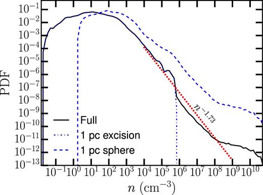
The probability distribution function of n. The black thin solid line shows the full PDF, the blue thin dot–dashed line shows the PDF with 1 pc spheres cut out around star particles, and the blue thin dash line shows the PDF within those spheres. The red dotted line show the power law ∝n−1.73.
The power law shows a break to a flatter slope at n ≈ 108 cm− 3. A similar break was seen by Kritsuk et al. (2011) who argued that at very high densities, the density PDF flattens due to the presence of discs which they also found. In our simulations, we have found that material with n > 109 cm−3 always resides within 0.01 pc of a star particle. Since 0.01 pc is the typical outer radius of our simulated discs, this suggests that the highest density material is strongly associated with the disc.
Fig. 11 shows the averaged vr, vT, vϕ, vK as a function of r before the star particle forms (left-hand panel) and after (right-hand panel). As in Fig. 9, we have selected the same fixed times (10 and 100 kyr) before the star particle forms and the same fixed masses (1 and 4 M⊙) after star particle formation. Here the dynamics of vT follow quantitatively the behaviour of vT found in MC15. In MC15, vT scales with radius as r1/2 at very large r, where self-gravity is not important. For example, at t = 100 kyr, before the star particle forms, we find that vT(r) ∼ r0.48, in line with Larson's law, i.e. ∝ r1/2.
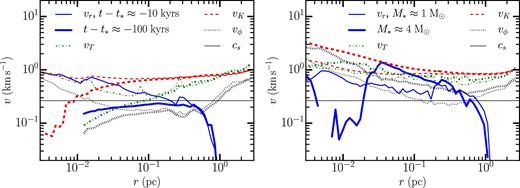
vr, vT, vϕ, and vK as a function of r at 10 000 (thin lines) and 100 000 (thick lines) yr before the star particle forms (left-hand plot) and when the star reaches 1 and 4 M⊙ (right-hand plot). The averages are over the same regions as those used in producing Fig. 9. The infall |ur| and random vT velocities show the behaviour predicted by the theory of adiabatic turbulent heating for times later than −10 000 yr: at large radii, where |ur| is small, vT > |ur| and vT decrease inwards, but more slowly than in non-collapsing regions; p ≈ 0.2 rather than p = 0.5. Inside r*, where |ur| > vT (or |H| > vT in the notation of Robertson & Goldreich 2012), vT increases towards |ur| as r decreases, with both increasing inwards.
However, at t = 10 kyr, before star particle formation, one can see that the vT scaling has reversed itself at small radii (r ≲ 0.1 pc) due to the accumulation of mass in a protodisc; the gas in the disc deepens the potential well, but does not provide radial pressure support. The figure also shows that |ur| increases inwards from r ≈ 0.1 pc.
The reversal of the power-law form of both |ur| and vT as a function of radius tracks the position of r*, as can be seen comparing the lines for t = −10 kyr in the left-hand plot with M = 1 and M = 4 M⊙ in the right-hand plot. This confirms another aspect of the MC15 solution – as r* moves outwards with time, the inflection point in |ur| and vT moves outwards as well, as we found earlier in Section 3.2.
The steady outward march of the sphere of influence is demonstrated in Fig. 12 which shows the run of enclosed mass at four different times. At t = −100 000 yr, in Fig. 9, the density cusp is not yet in place; correspondingly, at small radii the enclosed mass is convex, curving down as r decreases. By t = −10 000 yr, cusp formation is complete and a small disc has formed, evidenced by a slight upward concavity in the enclosed mass profile inside 0.02 pc. The radial extent of this upward concavity is increased to r ≈ 0.1 pc for M* = 1 and further to r ≈ 0.3 pc by the time the stellar mass reaches M* = 4 M⊙. The position of r* can be inferred by the position in the curves where the concave portion of the curve meets the linear portion. The concave regions are dominated by a central mass and hence are inside of r*.
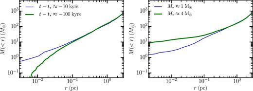
Mass of the gas and stars as a function of r at 10 000 (thin lines) and 100 000 (thick lines) yr before the star particle forms (left-hand plot) and when the star reaches 1 and 4 M⊙ (right-hand plot). Averages are as described in Fig. 9.
The growth of the central mass forces r*(t) outwards because ρ(r) is independent of time and hence the gas mass at small radii remains fixed, while M*(t) grows.
Returning to the velocities, the fact that vT(r) ∼ r0.48 for t = −100 kyr in the left-hand plot of Fig. 11 shows that the turbulence in the initial collapse obeys the same scaling law found in non-collapsing regions in the molecular cloud (Lee et al. 2015). This suggests that the turbulence in incipient collapsing regions is governed by the same large-scale turbulent cascade as in non-collapse regions.
However, the flattening and reversal of vT(r) at small radii and late times shows that some mechanism other than a turbulent cascade is at work at these radii and times. We interpret the behaviour of vT(r) as the combined result of compressional heating and turbulent decay, as suggested by MC15 and by Robertson & Goldreich (2012).
The relatively large infall velocity demonstrates that even 100,000 yr before the protodisc or star particle forms, these regions are not in hydrostatic equilibrium, in which the Reynold's stress or turbulent pressure balances the force of gravity. This calls into question the assumption made by previous analytic models of massive star formation, such as the turbulent core model. At early times, |ur| is between vK/3 and vK, except at r ≳ 1 pc where the clump fades into the ambient molecular cloud. These high ratios of |ur|/vK show that hydrostatic equilibrium is not a valid description of the star-forming regions at any time.
In fact, these plots show that |ur| is of the order of vK/3 or larger at all times for rd ≲ r ≲ 1 pc.
At small radii, the fact that ρ(r, t) = ρ(r) ∼ r−3/2 for r < r*, combined with the fact that |ur(r, t)| ∼ r−1/2, ensures that |$\dot{M}(r,t)=\dot{M}(t)$|, i.e. the mass accretion rate is independent of radius for r < r*.
This result for the accretion rate was shown previously in Fig. 7. At early times, (t − t*) ∼ −100 kyr (the red dotted curve), |$\dot{M}$| decreases by a factor of 20 between r = 0.5 and 0.01 pc because the density profile is still evolving towards the attractor solution. But for later times, |$\dot{M}(r)$| is flat at small radii. This demonstrates that the attractor solution, once established, imposes a major effect on the accretion profile.
While the gas is never hydrostatic, the gradient of the Reynolds stress does roughly balance gravity as can be seen in Fig. 13. The figure shows the rotational support which we define as |$v_{\phi }^2/r$| (solid blue line), Reynolds stress plus thermal pressure support, |$\rho ^{-1}\text{d}P/\text{d}r = \rho ^{-1}\text{d}\rho (v_{\rm T}^2/2+c_{\rm s}^2)/\text{d}r$| (dashed line), and total pressure support |$\rho ^{-1}\text{d}P/\text{d}r + v_\phi ^2/r$| (thick red line). We have scaled these quantities to the local gravitational acceleration, g = GM(< r)/r2.
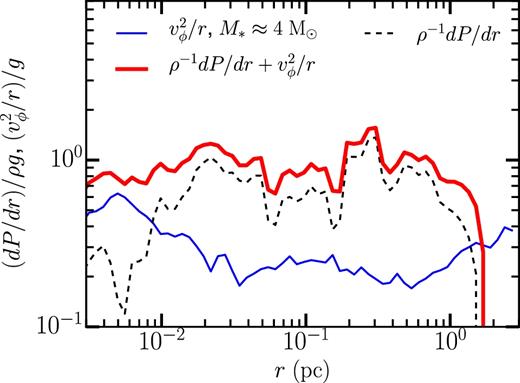
The ratio of rotational (solid line) support, Reynolds stress, and gas (dashed line) pressure support to the local gravitational acceleration g = GM( < r)/r2, as a function of r when the star reaches 4 M⊙.
Inside of r ≈ 0.01 pc, the gas settles into a rotationally supported disc and the support from other sources drops. However, the sum of the Reynolds stress and rotational support (thick red line) nearly balances the local gravity.
The rotationally supported discs in our simulations are, on average, roughly marginally stable, as seen in Fig. 14 which should be compared with fig. 3 in Kratter et al. (2010). For |$0.007\,\rm pc\lesssim \text{{r}} \lesssim 0.02\,\rm pc$|, we find 1 ≲ Q ≲ 1.6. Examining individual discs, some of the time the disc is unstable and rapidly dumps material towards the central star, while at other times the disc is stable, building up material to approach marginal stability. For r ≳ 0.02 pc, Q rises, though the interpretation of Q as a measure of stability is questionable, as the gas is no longer rotationally supported, nor is it in a flattened or disc-like configuration.
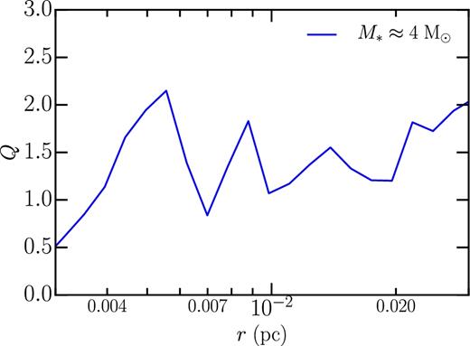
The average (over many discs) of Toomre Q as a function of r when |$M_{\ast }\approx 4\,\text{M}_{{\odot }}$|.
3.8 Mass accretion rates
Finally, we discuss the mass accretion rates in our simulation. Previously, Lee et al. (2015) (see also Myers et al. 2014) found that the SFE is non-linear in time, with M*∝t2. This non-linear rate is evident in the work of previous workers, but was often interpreted as an initial transient (Padoan & Nordlund 2011). MC15 showed that M*(t) ∼ t2 is a natural consequence of the density approaching an attractor solution and the scaling of the infall velocity with the Keplerian velocity at small radius, as we have clearly demonstrated in this work.
First, we address the question of whether the M*∝t2 phase is an initial ‘transient’. Tackenberg et al. (2012) and Traficante et al. (2015) estimate the lifetimes of massive star-forming clumps found using the Apex telescope and the Herschel telescope, respectively. Tackenberg et al. (2012) identify clumps with column densities |$\Sigma _{\rm g}> 0.1\,\rm g\,\rm cm^{-2}$|, masses up to 105 M⊙. Since they have a fairly complete catalogue of such clumps, they can estimate the typical lifetime of a clump by comparing to the number of massive stars formed in the Milky Way every year. They find a mean clump lifetime of 6 × 10⁴ yr and a clump free-fall time of ≈ 1.5 × 10⁵ yr; the clumps live one free-fall time.
Similarly, Traficante et al. (2015) identify clumps with sizes ranging from |$0.1\text{ to }1\,\rm pc$|, masses ranging up to 104 M⊙. They estimate an upper limit lifetime for the starless phase of 105 yr for clumps with M > 500 M⊙ and a ratio of starless to total clumps (the rest of the clumps host protostars) of 39 per cent. Thus, the total lifetime of clumps in their mass range (above 500 M⊙) is |${\sim } 2\text{--}4\times 10^5\,\rm yr$|. The clumps in their sample have |$10^4\,\rm cm^{-3}\lesssim \text{{n}}_H\lesssim 10^5\,\rm cm^{-3}$|, so free-fall times |$1.6\times 10^5\,\rm yr\lesssim \tau _{ff}\lesssim 5\times 10^5\,\rm yr$|. The clumps live 0.2–2.5 free-fall times, similar to the estimate of Tackenberg et al. (2012).
Thus, the lifetimes of massive star-forming clumps, when measured in units of free-fall times, are similar to the lifetimes of GMCs, again measured in free-fall times, e.g. Blitz et al. (2007) who find that GMCs live two to three free-fall times.
Our simulations run for only a fraction of a free-fall time, but those of other workers have often run for two to three (Wang et al. 2010; Padoan & Nordlund 2011) or, in some cases, up to five free-fall times. The simulations are often halted when ∼10–30 per cent of the mass has been converted into stars, since that is a rough observational estimate of the maximum fraction of clump gas turned into stars, e.g. Lada & Lada (2003). In most cases, this SFE is reached in one or two free-fall times, while the M*(t) ∼ t2 behaviour is still apparent from the plots. In the case of Federrath (2015), in the magnetohydrodynamic (MHD) run with stellar wind/jet feedback, the M(t) ∼ t2 behaviour ceases after four free-fall times, when the SFE is about 15 per cent. Since it is unlikely that star-forming clumps live so long, the simulated star formation rate is probably too low.
We conclude that the time-scale over which the t2 scaling is seen in simulations is similar to the lifetimes of massive star-forming regions, so that while the behaviour we focus on may be of short duration, it is not ‘transient’.
In Fig. 15, we show the total M* as a function of time since the first star particle was formed, t*. This is exactly the same analysis as Lee et al. (2015). However, because the simulations are distributed among the eight different octants, each with a different star formation time, we produce the total SFE history as follows. First, we analyse the simulations to find the earliest time at which a star particle formed, which we define as t*. We then look at all the simulation to find the earliest time at which a simulation ended or tend, which defines the time over which all our simulations have data. Because each snapshot for each simulation is taken at different times, we define a number of times at fixed intervals between t* and tend and interpolate the total stellar masses for each simulation on those times. These masses are then summed to produced M*(t), which we plot in Fig. 15.
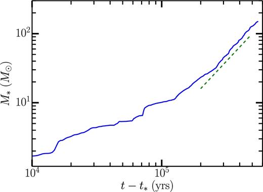
The total mass in stars plotted as a function of time since the first star particle formed, t*. The final value of the total stellar mass |$M_{\ast }\approx 180\,\text{M}_{\odot }$| is about 1 per cent of the total gas mass in the box, while the final t − t* ≈ 0.6 Myr, about 15 per cent of the free-fall time 3.8 Myr for the mean density of the box. The dashed green line shows a slope of 2.
As shown in Fig. 15, M*(t) grows roughly linearly for ≈ 100 000 yr after the first star particle is formed. However, once the total stellar mass reaches about |$M_{\ast } \gtrsim 10\,\text{M}_{{\odot }}$|, at a time t − t* ≳ 100 kyr, M*∝t2. At this stage, M*/MGMC ∼ 0.001. This agrees well with the results of Lee et al. (2015) who found M* ∼ t2 for stellar masses between M*/MGMC ≈ 0.015 and 0.3. Due to the computationally expensive nature of our much higher resolution simulations, even given the use of AMR, we are not able push our simulation to the same total M*/MGMC as Lee et al. (2015) were able to in their fixed grid, but much lower resolution simulations. However, our simulations do show that their simulations were already at sufficiently high spatial resolution to recover the scaling relation.
The reason for this is not hard to find. Fig. 9 shows that at r ≈ 1 pc, the density has already settled on to its time-independent form, while Fig. 11 shows that the infall velocity is scaling as r−1/2 for |$r\lesssim 0.3\text{--}0.7\,\rm pc$|, with the smaller value corresponding to the time of star particle formation and the larger value to times for which |$M_{\ast }\approx 1\,\text{M}_{\odot }$|. As long as a simulation resolves this radius (which corresponds roughly to r*), it will recover the M* ∼ t2 scaling.
The slower growth at earlier times is due to fact that at the time of star formation, the infall velocity is non-zero, despite there being no star to attract the gas; see Fig. 11. In other words, the initial infall velocity is larger than |$\sqrt{GM_{\ast }/r}$|; it takes time before the Reynolds stress can slow the infall to the steady state value given by equation (4) and hence before the mass accretion rate settles on to the steady state value given by equation (5).
The same comments apply to the accretion rates of individual stars; individual stars start accreting out mass at a roughly constant rate. At later times, when they have substantial masses, the accretion rate grows linearly in time. This happens only with the most massive star particles in our simulation.
The total number of star particles also grows roughly linearly with time; the combination of this linear growth in number of stars, together with the roughly linear mass growth of most of the stars, produces the overall M* ∼ t2 scaling we see for the simulation region as a whole. In regions where the summed accretion rate is highest, individual star particles are not able to accrete all the collapsing mass, leading to the formation of new star particles in the immediate vicinity. In other words, our simulations produce clustered star formation. This is similar to what has been found in other recent simulations (Gong & Ostriker 2015; Lee et al. 2015).
We interpret equations (3)–(5) as a description of star cluster formation; the total mass of the cluster will grow as t2; the most massive stars may spend a significant fraction of their accretion history growing as t2, but many of the less massive stars will not undergo such rapid growth in their accretion rate.
4 DISCUSSION
4.1 Basic results of this work
We begin with a summary of our results.
4.1.1 Collapse is not self-similar
First, in our isothermal, driven turbulence simulations, star formation is not a self-similar process. Two length-scales, in addition to the radius of the outer boundary condition or turbulence outer scale and the stellar radius, enter the problem. The outer disc radius rd which is the radius at which the gas becomes rotationally supported and the radius r* of the stellar sphere of influence, i.e. the smallest radius at which the gravity of the gas dominates the gravity from the star and disc. The existence and significance of rd has been known since the time of Kant and Laplace; the recognition that r* plays a role in star formation is recent, so we concentrate on the effect of r* on the dynamics in what follows. The value of r* increases monotonically with time, since the stellar mass increases monotonically, while rd may vary in or out with time, depending on the (turbulently determined) distribution of angular momentum of the accreting gas.
The non-self-similar behaviour of the collapse is most strongly reflected in the variation of vT with radius; for rd < r < r*, the random motion velocity is a decreasing function of radius vT(r) ∼ rp with p ≈ −1/2, while for r* < r, it is an increasing function of r, scaling like r0.2. Similarly, the infall velocity |ur| ∼ r−1/2 for rd < r < r*, while for r* < r, it is flat or even increasing outwards (as in the top panel of Fig. 5), with substantial variations both from particle to particle and at different times for the same particle, due to the vagaries of the turbulent flow at large radii.
4.1.2 Density approaches an attractor solution
Secondly, we find that inside the sphere of influence of the star, the density remains constant over several to tens or even hundreds of (local) dynamical or infall times; for rd < r < r*, ρ(r, t) → ρ(r). This is illustrated by Figs 6 and 9. One implication of this result is that one cannot use observations of the free-fall or crossing time of collapsing structures to infer either the age or lifetime of those structures.
The fact that ρ(r, t) = ρ(r) ∼ r−3/2 for r < r*, combined with the fact that |ur(r, t)| ∼ r−1/2, ensures that |$\dot{M}(r,t)=\dot{M}(t)$|, i.e. the mass accretion rate is independent of radius for r < r* (see Fig. 7).
Since |ur| increases with stellar mass and hence with time where r < r* (see the second panel in Fig. 11), while ρ is fixed, |$\dot{M}(t)$| increases with time, a result seen in many previous papers (Padoan & Nordlund 2011; Bate 2012; Federrath & Klessen 2012; Krumholz et al. 2012b; Myers et al. 2014), although this fact was usually not commented on. After some initial transient behaviour, we find M(t) ∼ t2 (Fig. 15) in line with the results of Lee et al. (2015).
4.1.3 Partitioning of the collapsing region's potential energy
Our third result is to show how the potential energy released in collapse is partitioned. In our simulations, the support from random motions slows the rate of infall, so that |ur| is significantly smaller than the free-fall velocity, but large enough to maintain vT at a sufficient level such that the acceleration due to the Reynolds stress is close to the acceleration of gravity (Fig. 13). In contrast, Sur et al. (2010) and Federrath et al. (2011) find an infall velocity which is equal to the free-fall velocity just outside their core. The dynamics in their simulation is very different to the dynamics in ours; in their case, the acceleration due to the pressure gradient is negligible compared to the acceleration due to gravity. Their initial conditions incorporate transonic turbulence, but no driving. Since the collapse in their simulation does not take place for roughly four free-fall times, by the time the collapse starts, the turbulence is subsonic.
Because the infall in our simulations is typically supersonic, some of the kinetic energy can then be converted into thermal energy by shocks; of course, even in the absence of shocks, normal (molecular) adiabatic heating will convert a small fraction of the liberated potential energy into heat.
Figs 3–5 show that for r > r*, the bulk of the potential energy goes into random motion and thence into shocks. Inside r*, but outside of the disc, the potential energy that is not immediately radiated is shared roughly equally between the infall and random motions. Inside of the disc, the potential energy is converted to rotational and random motion, in roughly equal measure, and thence to thermal emission. At any radius, the ratio of kinetic energy to potential energy is typically around a quarter to a half, although at large radii (r ≳ 1 pc), the turbulent kinetic energy can exceed the potential energy: on the scale of our box, the ratio |$v_{\rm T}/\sqrt{GM_{\rm GMC}/r_{\rm GMC}}\approx \alpha ^{1/2}_{\rm vir}\approx 1$|, where MGMC is the total mass contained in the simulation volume and rGMC = 8 pc is the ‘radius’ of the simulation volume, i.e. half of the side of the box. This ratio scales as |${\sim } 1/\sqrt{r}$|, so at r ≈ 1 pc, the ratio is |${\sim }\sqrt{8}$|.
We also found evidence that the ratio of radial to transverse random motion depends on whether the collapse leads to radial compression (for r > r*) or dilation (for r < r*) and on the tendency for hydrodynamic turbulence to isotropize motions down the cascade; see Fig. C2 and the discussion in Section C1.
4.1.4 Modification of Larson's law
Our fourth result is the confirmation that the adiabatic heating of the turbulence alters Larson's law. On large scales or away from collapsing regions, Larson's law is vT ∼ rp with p ≈ 0.4–0.5. It emerges naturally from the decay of supersonic turbulence which is driven on large scales. We find, as did Lee et al. (2015), that in rapidly collapsing regions, the decay of vT ∼ rp with decreasing radius is slowed for r* < r ≲ 1 pc. Least-squares fit to vT(r) for over this range of radii result in exponents within the range 0.1 ≲ p ≲ 0.4, with an average around p ≈ 0.2, in fair agreement with the prediction of equation (4). Inside of r*, we find p = −1/2, as predicted by equation (4), representing a reversal of Larson's law.
4.1.5 Collapse does not proceed in an inside-out manner
A fifth result is that the gathering and accretion of mass starts from large scales and both before and after a star particle forms, |$\dot{M}(r,t)$| is larger at large r than it is at small r; in other words, the collapse proceeds in an outside-in manner. The first point that the accretion starts from large scales is illustrated by Figs 2 and 3 and the left-hand panel of Fig. 11, which show that |ur(r)| ∼ (1/3)vK(r) out to r ∼ 1 pc or farther and is trans- or supersonic tens or hundreds of thousands of years before the density cusp forms and hence before star or even disc formation starts.2
Fig. 7 shows that just after the cusp/star particle forms, the mass accretion rate is actually larger at larger radii. This behaviour is the opposite of that predicted by inside-out collapse models, either that of Shu or of the turbulent core model. In Fig. 7, this inside-out behaviour is illustrated with a Shu-type solution, shown by the dashed line; in that solution, the mass accretion rate decreases with increasing radius, in contrast to the results of our simulation.
Figs 5 and 11 (right-hand panel) show that just after and well after the star forms, the surrounding region is also far from hydrostatic equilibrium.
We conclude that there is no indication of gas in hydrostatic equilibrium prior to, during, or after star particle formation in our simulations, nor is there any indication of inside-out collapse.
The violation of self-similarity and evidence against inside-out collapse shows that the assumptions made by previous analytic collapse models (Shu 1977; Myers & Fuller 1992; McLaughlin & Pudritz 1997; McKee & Tan 2003) are not fulfilled in our simulations. In addition, the collapsing regions in our simulations do not start from a hydrostatic equilibrium.
4.1.6 The magnitude of the pressure gradient term is comparable to that of the gravity term for r > rd
Fig. 13 shows that the acceleration due to the pressure gradient is comparable to the acceleration of gravity for rd < r < r*. Thus, Reynold's stresses slow the infall compared to the free-fall rate, i.e. |$|u_{\rm r}(r,t)|< \sqrt{GM(r)/r}$|. At small radii (r < rd), the rotational support becomes important and the support from vT becomes much smaller than the radial component of gravity, but comparable to the vertical component in the disc.
4.1.7 The total stellar mass increases as t2
The total stellar mass in our simulation region, and in individual star-forming sub-regions, increases as the square of time after the first star (in the box or in the individual star-forming region) forms. Low-mass (less than a few solar masses) stars have M*(t) ∼ tγ, with 0 ≲ γ ≲ 2, with a typical value γ ≈ 1 but the total number of low-mass stars N(t) ∼ t, so that the total mass in low-mass stars grows as t2. High-mass stars which tend to sit at density peaks (or at the bottom of potential wells) have M*(t) ∼ t2.
4.2 Comparisons to observations
Caselli & Myers (1995) showed that massive star-forming regions have shallower linewidth–size relations than the classical Larson result, i.e. vT(r) ∼ rp with p = 0.21 ± 0.03, compared to p ≈ 0.53 ± 0.07 in low-mass star-forming regions. Plume et al. (1997) also found that Larson's law breaks down in massive star-forming regions, i.e. their measured linewidths are larger for a given source size than those found in low-mass star-forming regions. As noted in Section 4.1.4, we find the same behaviour in our simulations and we interpret this as the effect of adiabatic heating in a collapsing flow at r > r*.
In addition, Plume et al. (1997) plotted the mean velocity dispersion as a function of number density which they derived from an excitation analysis of CO. They found that contrary to expectations, the velocity dispersion increased with increasing density, which is opposite to the expectation based on Larson's law or supersonic turbulence driven from large scales. They concluded that the conditions in dense star-forming cores are different from the rest of the cloud. The simulations presented here and the analytic results of MC15 show the same behaviour. In particular, the theory suggests that the enhanced turbulence or velocity dispersion at small radii in dense star-forming regions is the result of gravitational collapse adiabatically heating the turbulence.
We find qualitative agreement between the observations of Plume et al. (1997) and our results, i.e. enhanced linewidths at high densities which are associated with smaller radii. Performing a more detailed comparison is more difficult as we have selected regions with the same stellar mass, whereas the stellar mass in Plume et al. (1997) is not well known. However, it is promising that the linewidths in our simulations are of similar magnitude and show the same trend with density as do the observations.
There are now numerous measurements of infall at large radii |${\sim } 0.1\text{--}1\,\rm pc$| in the literature. For example, Csengeri et al. (2011) examine DR21 in Cygnus X. They see infall |$|u_{\rm r}|=0.1\text{--}0.6\,\rm km\,s^{-1}$|, |$\sigma _{\rm T}\sim 0.6\text{--}2\,\rm km\,s^{-1}$| at n ∼ 105–106, r ≈ 0.1 pc. Other examples include Ragan et al. (2012, 2015) and Peretto et al. (2013).
Infall is also seen on larger scales, r ≈ 1 pc, by Wyrowski et al. (2016) who observe |ur| in the range |$0.3\text{--}3\,\rm km\,s^{-1}$|, corresponding to a fraction of the free-fall velocity (1.4 times the Keplerian velocity) of 0.03–0.3. In other words, the gas at r = 1 pc is not in hydrostatic equilibrium, nor is it in free fall. The turbulent velocity in the same clumps at the same radii is comparable or slightly in excess of the infall velocity, |$v_{\rm T}\approx 1.0\text{--}2.3\,\rm km\,s^{-1}$|.
Ho & Haschick (1986), Klaassen & Wilson (2008), and Klaassen et al. (2011) see infall at three different radii, r ≈ 0.5, 0.3, and 0.03 pc using different molecular tracers in the same object, G10.6-0.4. The infall velocity is large at r, small at r ≈ 0.3 pc, and large again at r ≈ 0.03 pc. As noted by MC15, this is in qualitative agreement with the picture of adiabatically heated turbulence.
4.3 Missing physics
Our current understanding of star formation suggests that the effects of magnetic fields, radiative and protostellar outflow feedback from stars, and the equation of state of the gas can all have significant effects on both the rate of star formation and the IMF of the stars. We do not include any of this physics in the simulations described in this paper.
It is often argued that the turnover in the IMF, somewhere between 0.2 and 0.6 M⊙, is associated with the thermal state of the gas in the collapsing region. If so, then our use of an isothermal equation of state suggests that the IMF found in our simulations is likely to be in error, so we have not discussed our computed IMF. However, as Figs 2–5 and 11 show, both |ur| and vT exceed cs, except at the earliest times ( ∼ 100 000 yr before a star forms) and then only for r ≲ 0.1 pc, so that the gas pressure does not dominate the dynamics in most regions and most of the time. Of course we do include the effects of gas pressure, so even in those regions and those times, our simulations capture the dynamical effects to lowest order aside from, as we have just said, the fragmentation effects on the smallest scales.
We have undertaken and made some preliminary analyses of MHD simulations, which we will report on in future publications; as seen by other authors, we find that magnetic fields slow the star formation rate. But the runs of density and velocity have the same qualitative form in our MHD simulations as in the hydro runs presented here and the MHD runs also give M*(t) ∼ t2.
Like magnetic fields, feedback from protostellar outflows are seen to slow the rate of star formation, e.g. Wang et al. (2010) and Federrath (2015). But those authors also find that |$\text{d}M_{\ast }/\text{d}t$| increases with time even in runs that include outflows.
Radiative feedback will also affect both the IMF and, for massive enough stars, the dynamics of the collapse at late times (after massive stars have formed).
All the figures we show present results for stars with masses no larger than about 4 M⊙. To estimate the effects of radiation, we compare the force from the Reynolds stress |$F_{\rm T}=4\pi r^2 \rho v_{\rm T}^2$|, to the radiation force L/c. From Fig. 11, the (averaged over many stars) vT is slightly in excess of 1 km s− 1 at r = 0.01 pc, while from any of the density figures, the density is ρ ≈ 5 × 10⁻¹⁸g cm−3. The force from Reynolds stress is then F ≈ 4 × 1026 dynes. The luminosity of a 4 solar mass star on the zero-age main sequence is L ≈ 2 × 1036 erg s− 1 (Schaller et al. 1992), so the radiation force L/c ≈ 3 × 1025 dynes, about a 10 per cent effect. The force from Reynolds stress increases outwards, see Fig. 13, so this statement holds at larger radii as well.
Thus, we expect that the effects of radiation pressure are not particularly significant in the situations we report; the run of density and infall velocity and hence the M*(t) ∼ t2 scaling should not be affected, at least up to the times we are reporting on. We note, however, that this estimate neglects the effect of radiative or ionization heating which is an important feedback mechanism.
Simulations including radiative feedback support this simple analysis. Fig. 15 of Myers et al. (2014) shows that in their simulations, which include feedback from both protostellar outflows and radiation (as well as magnetic fields), the stellar mass increases as the square of the time, up to masses of 4.5 solar masses. Earlier work by the Berkeley group found similar results, forming stars with 10 solar masses, with M*(t) t2 even for such massive stars; see fig. 13 of Krumholz et al. (2012b). Their simulations included radiative effects, but no protostellar winds.
5 CONCLUSIONS
Motivated by recent analytic (MC15) and numerical (Padoan, Haugbølle & Nordlund 2014; Lee et al. 2015) results, we perform deep AMR simulations of star formation in self-gravitating continuously driven hydrodynamic turbulence. We show that two length-scales emerge from the process of star formation, r* and rd, and demonstrate that these length-scales are clearly associated with physical effects. In particular, the character of the solution changes at r*(t), inside of which (but outside rd) |ur| and vT are both ∝r−1/2; outside of r*, vT ∼ rp (with p ≈ 0.2), while |ur| is on average about constant. We emphasize that the length-scales at which the character of the solution changes are time-dependent. As the star grows in mass, the radius where the stars’ gravity exceeds the gravity of the surrounding gas increases outwards away from the star, |$r_{\ast }(t) \propto M_{\ast }^{2/3}(t)$|. The disc radius, rd, also changes as a function of time as a result of the advection and transport of angular momentum from large scales to small scales (and vice versa).
We also found that the density profile evolves to a fixed attractor, ρ(r, t) → ρ(r), in line with the results of MC15 and the earlier numerical results of Lee et al. (2015).
Our results strongly support the basic premise of MC15 that turbulence is a dynamic variable which is driven by adiabatic compression (Robertson & Goldreich 2012) and that the turbulence in turn acts to slow the collapse. We note, as did MC15, that observations of massive star-forming regions also find vT ∝ rp with p ∼ 0.2–0.3, and at small radii or high density, vT increases with increasing density, as seen in observations of massive star-forming regions (Plume et al. 1997). We find these departures from Larson's law only in collapsing regions in our simulations. We also show that the acceleration due to the pressure gradient is comparable to that due to gravity at all r > rd. As a result, the infall velocity is substantially smaller than the free-fall velocity even very close to the star or accretion disc. Inside rd, rotational support takes over and as a result, ur and vT both decrease.
Our simulations capture rotational dynamics that MC15 did not capture in their 1D model. In particular, we find the development of rotationally supported discs at rd ∼ 0.01 pc. These discs have radii comparable to or slightly larger than discs seen around young stars in Taurus (Padgett et al. 1999) in which stellar feedback effects are minimal and where the undisturbed discs are larger than in more active star-forming regions such as Orion, where the disc radii are ∼100 au (Williams & Cieza 2011). This is despite the fact that we do not include magnetohydrodynamic effects in our numerical computations; large-scale magnetic fields may transfer angular momentum away from these discs, shrinking them.
Like the discs modelled by Kratter et al. (2010), our simulated discs are marginally gravitationally stable, suggesting that large-scale gravitational torques are responsible for transport of material and angular momentum in our simulations; this may also be true at early times in real protostellar discs.
We have shown that the assumptions made by previous analytic collapse models (Shu 1977; Myers & Fuller 1992; McLaughlin & Pudritz 1997; McKee & Tan 2003) are not fulfilled in our simulations. In particular, the collapsing regions in our simulations do not start from a hydrostatic equilibrium, nor do they show any evidence of inside-out collapse. The gathering of material before collapse, i.e. before the central cusp in the density power law is formed, involves transonic bulk motions and supersonic random motions (see Fig. 11). The accretion of mass starts at large scales (r ∼ 1 pc) with large initial infall velocities. In addition, we find that vT scales differently in collapsing regions as opposed to the rest of the simulation box, whereas the turbulent collapse models (McLaughlin & Pudritz 1997; McKee & Tan 2003) assume that the scaling of vT with r remains fixed.
Finally, we close with a brief discussion of how our results relate to turbulence-regulated theories of star formation. Here we find several points of disagreement. First, we find that the star particles accrete continuously from the surrounding large-scale turbulent flow; there is no hydrostatic ‘core’ which is cut-off from the turbulent medium. Secondly, the density distribution does not remain lognormal, but rather develops a power-law tail that is directly related to the density profile (Kritsuk et al. 2011; Lee et al. 2015). Thirdly, the fact that the density profile approaches an attractor solution which scales like r−3/2 for r < r* and ur scales with the Keplerian velocity guarantees that |$\dot{M}$| is constant with radius and |$\dot{M}_{\ast }\propto t$| and hence a non-linear SFE, i.e. M*∝t2 results. This is in contrast with turbulence-regulated theories of star formation which predict a constant star formation rate, i.e. |$\dot{M}_{\ast } = {\rm const}$| and hence a linear SFE, M*∝t.
Acknowledgments
We would like to thank the anonymous referee for useful comments. DM, PC, and JP are supported in part by the NASA ATP program through NASA grant NNX13AH43G, NSF grant AST-1255469, and the Research Growth Initiative at the University of Wisconsin-Milwaukee. NM is supported by the Canada Research Chair program and by NSERC of Canada. Some of the computations were performed on the gpc supercomputer at the SciNet HPC Consortium (Loken et al. 2010). SciNet is funded by: the Canada Foundation for Innovation under the auspices of Compute Canada; the Government of Ontario; Ontario Research Fund – Research Excellence; and the University of Toronto. The authors also acknowledge the Texas Advanced Computing Center (TACC) at The University of Texas at Austin for providing HPC resources that have contributed to the research results reported within this paper. URL: http://www.tacc.utexas.edu. This work was performed in part at the Aspen Center for Physics which is supported by National Science Foundation grant PHY-1066293.
The gas in the disc around the protostar is rotationally supported, so it essentially acts as a part of the star. We include the mass of the disc when calculating r* and discuss how we define the disc mass in 3.5.
We remind the reader that the scale of the infall region in our simulations, and possibly in the ISM of galaxies, is simply a fraction of the driving scale of the turbulence.
Note that we define vT, l as an average so that we can compare it directly to vT, r.
REFERENCES
APPENDIX A: CALCULATING THE RANDOM MOTION AND ROTATIONAL VELOCITY
In this appendix, we discuss how we calculate the random motion, vt, infall, ur, and rotational velocities, vϕ from the full 3D numerical solution. To begin, we adopt a series of concentric, logarithmically spaced, spherical shells around either a star particle (if available) or around a density maximum in the case where the star particle has not yet formed. We then removed the bulk velocity from these shells by first calculating the enclosed mass, M(< r), and momentum in each sphere |${\boldsymbol P}(<r)$|, then dividing the two to find the bulk velocity, |${\boldsymbol V} = {\boldsymbol P}(<r)/M(<r)$| of the sphere of matter. We then subtract this bulk velocity from the corresponding shell.
We also tried defining the bulk velocity using the total momentum in each of the spherical shells (rather than in the enclosed spheres) and found very similar results.
We then subtract the bulk velocity from the raw velocity of each cell in the spherical shell. We denote the result by |${\boldsymbol v}$|.
APPENDIX B: FILAMENTARY OR SPHERICAL ACCRETION?
Figs 2–5 show that the density in the vicinity of collapsing regions is decidedly non-spherical. Despite this, the results of MC15 appear to describe the accretion process well. For example, in those same figures, we have shown mass-weighted infall, random motion, and rotational velocities, the first two of which behave as predicted by MC15 (they made no predictions for vϕ).
To understand this better, we examine how |$\dot{M}$| depends on ρ and how both are distributed on the sky as seen by the accreting particles. The left-hand plot of Fig. B1 shows a histogram of cumulative |$\dot{M}(\rho )/\dot{M}_{\rm tot}$| through two spherical shells at r = 0.5 pc and 0.05 pc, as a function of ρ/〈ρ〉, where 〈ρ〉 denotes the density average over the (finite thickness) shell. We show average histograms when the central star has a mass M* = 1 (dashed lines) and 4 M⊙ (solid lines). The plot shows that 50 per cent of the accretion through the sphere occurs via the gas that has a density less than two–five times the average density of the shell, where the low end of this range occurs at small radii at late times, with the high end occurring at large radii and early times.
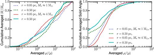
Histogram of the cumulative normalized |$\dot{M}$| (left) and cumulative normalized solid angle (right) as a function of normalized density for r = 0.05 and 0.5 pc when the star reaches 1 and 4 M⊙.
Since the mean density at r = 0.5 pc is |$\langle \rho \rangle \approx 3\times 10^{-21}\,\rm g\,\rm cm^{-3}$|, see Fig. 6 or Fig. 9, an examination of Fig. 5, where the gas with three times the mean density is depicted by dark green (and less dense gas is blue), shows that more than half of the accretion is coming from the gas that covers most of the sky as seen from each of those accreting particles; most of each slice is coloured blue. If we take filaments to consist of the gas which is coloured light green or yellow (with ρ > 10−20 or ∼3 times the mean density 〈ρ〉 inside r = 0.5 pc), the filaments account for less than half the accretion.
A similar statement holds for the accretion inside r = 0.05 pc, shown as the thin lines in Fig. B1.
To see more quantitatively how this gas is distributed on the sky, we plot in the right-hand panel of Fig. B1 the cumulative solid angle as a function of ρ/〈ρ〉, again for r = 0.5 pc (thick lines) and for r = 0.05 pc (thin lines). Roughly 90 per cent of the sky is covered by the gas that is at three times the average shell density or lower, consistent with the qualitative analysis in the previous paragraph.
Fig. B2 shows a histogram of the cumulative normalized |$\dot{M}$| as a function of the cumulative normalized solid angle. The plot shows that half the accretion occurs over about 10 per cent of the sky where the density is ∼3 or more times the mean density of the spherical shell. So, while about half the gas accretes from over most of the sky and at about the mean density, very dense gas entering the sphere from a very small covering fraction of the sky contributes the other half of the total accretion budget.
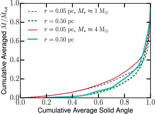
Histogram of the cumulative normalized averaged |$\dot{M}$| as a function of the cumulative normalized averaged solid angle for r = 0.05 and 0.5 pc when the star reaches 1 and 4 M⊙.
Thus, while the filaments are readily identifiable by eye and are important sources of accreting gas, much of the accretion (and much of the mass) lies in gas which is more nearly spherically distributed.
APPENDIX C: STAR FORMATION CRITERIA
The majority of our simulations used a simple density condition of three times the Truelove condition (equation 8) at the maximum refinement level inspired by the sink particle formation criteria of Padoan & Nordlund (2011) as discussed in Section 2. We have experimented with additionally including the sink particle checks of Federrath et al. (2010b) to check the robustness of our results to these additional checks. In Fig. C1, we show the run of velocity in a simulation in which we included the star particle formation checks used in the default used in flash. The results do not differ significantly from runs lacking such checks. For example, both show that the stellar mass increases like t − t* squared, M*(t − t*)∝(t − t*)2. There are however stochastic variations in the stellar mass ratio from runs with and without the extra checks. The mass ratio at a given (t − t*) can vary by a factor of roughly 2. For example, a hundred thousand years after the first star forms, in one run, the total stellar mass is 10 M⊙, while in another, it is 15 M⊙.
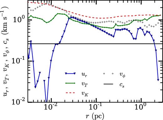
The run of velocity for a particle formed in a simulation using flash's built-in particle formation checks (as well as the density condition proposed by Padoan & Nordlund 2011). This shows that the dynamics of collapse are not overly sensitive to the star particle creation algorithm.
C1 Radial and lateral components of the random motion velocity
Fig. C2 shows the radial vT, r and lateral vT, l ≡ (vT, θ + vT, ϕ)/23 components of the random motion velocity for the same collapsing region as shown in Fig. 5, where vT, θ and vT, ϕ are the random motion velocities along the |$\hat{\theta }$| and |$\hat{\phi }$| directions defined from the z-axis. In the absence of self-gravity, a turbulent hydrodynamic cascade to small scales tends towards equipartition, (vT, r ≈ vT, l), with a scaling behaviour vT ∼ r1/2, similar to that seen in Larson's size–linewidth relation; this is what we see in non-collapsing regions in our simulation.
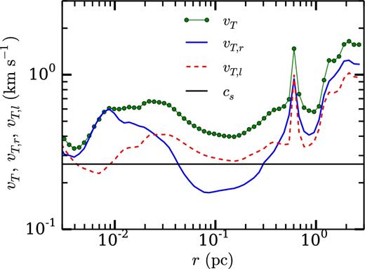
The radial vT, r (blue solid), lateral vT, l = (vT, θ + vT, ϕ)/2 (red dashed) and total (green line overplotted with dots) random motion velocities as a function of radius for particle B 100 000 yr after the particle formed. The sound speed cs is shown for comparison (black horizontal line). At large radii, vT, r ≈ vT, l; for |$0.04\,\rm pc\lesssim r\lesssim 0.4\,\rm pc$|, vT, r < vT, l, while inside of 0.03 pc, vT, r quickly recovers and then exceeds vT, l. The behaviour of the lateral and radial velocities is dictated by the radial infall velocity in Fig. 5 (see the main text).
Fig. C2 shows that both the radial and transverse components of the random motion velocity decrease with decreasing r for 0.4 ≲ r ≲ 3 pc (except for a spike at r ≈ 0.6 pc). Furthermore, the ratio vT, r/vT, l ≈ 1. We interpret the decrease as the decay of turbulence down a cascade. However, the decrease in both the total and in the longitudinal component, when fit with a simple power law, gives vT ∼ rp with p = 0.2, while the decrease in the radial component of the turbulence corresponds to p ∼ 0.35. Since both exponents are less than the value p ≈ 0.5 that we see on larger scales or away from collapsing regions, we conclude that adiabatic heating is affecting both the radial and transverse components of the turbulence.
At smaller radii, |$0.04\,\rm pc\lesssim \text{{r}}\lesssim 0.4\,\rm pc$|, the inward decrease of both vT, r and vT, l slows and then reverses, as the flow passes r*. However, the ratio vT, r/vT, l is now only 1/2. Finally, at and inside the disc radius rd ≈ 0.02 pc, the lateral turbulence once again decreases inwards, while the radial component grows until much smaller radii, before decreasing again.
If adiabatic heating is responsible both for the slower than normal decrease with random motion velocity at r > r* and for the increase in random motion velocity inside r*, why does the ratio of the radial and lateral components of the turbulence vary?
In Fig. 5, |$|u_{\boldsymbol r}|$| is decreasing with decreasing radius over the range |$0.4\,\rm pc\lesssim \text{{r}}\lesssim 3\,\rm pc$|. What this decrease means physically is that as the gas falls in towards the centre, it is being compressed not just in the θ and ϕ directions, but also radially. This compression along the radial direction should drive radial turbulence, while the lateral compression should drive lateral turbulence. This is why the radial and lateral components of the random motion velocity have the same magnitude.
This physical reasoning also tells us that as the infall velocity increases inwards over the range |$0.04\,\rm pc\lesssim \text{{r}}\lesssim 0.4\,\rm pc$| (see Fig. 5), the gas dilates in the radial direction even as it continues to compress in the transverse (θ and ϕ) directions. Compression in the θ and ϕ directions will tend to drive an increase in the lateral components of the random motion velocity, but dilation in the radial direction will tend to drive a decrease in the radial component; of course, both tendencies have to compete with (or add to, in the case of radial motion) the usual tendency for turbulence to decay, and the tendency, mentioned above, for hydrodynamic turbulence to tend to equipartition as the motion cascades to small scales.
We interpret the rapid inward decline of vT, r starting at r ≈ 0.4 pc as the effect of adiabatic cooling. The result is that the ratio vT, r/vT, l ≈ 1/2 for |$0.04\,\rm pc\lesssim \text{{r}}\lesssim 0.4\,\rm pc$|.
Between rd ≈ 0.02 pc and the local maximum of |$|u_{\boldsymbol r}|$| at r ≈ 0.04 pc, the infall velocity is large but roughly constant, meaning that the radial dilation ceases. We interpret the uptick in vT, r towards small radii as the result of the cascade of vT, l driving the radial component, as the turbulence strives to reach equipartition, combined with the cessation of adiabatic cooling associated with the cessation of radial dilation.
Inside r ≈ 0.02 pc, the infall takes place primarily through a rotationally supported disc, in which both the vertical vT, θ and azimuthal vT, ϕ components of the turbulence are greatly reduced (although we do not show the separate components in the figure). At the outer edge of this disc, we see a sharp rise in the radial component of the random motion velocity, followed at yet smaller radii by a decrease in the total turbulent velocity. We interpret the drop in the total turbulent velocity at small radii as the flow settling into more ordered motion in an accretion disc.
APPENDIX D: THE INITIAL MASS FUNCTION
For completeness, we report the IMF in this subsection, though we caution the reader again that because we do not handle the thermal physics properly, the location of the break in the IMF is unlikely to be correct; however, it is commonly believed that the slope at the high-mass end is set by the turbulence so that the thermal properties will not have much effect there. Fig. D1 shows the IMF at the end of our ramses run with NJ = 32. The plot includes a total of 90 stellar particles, with a total mass of 240 M⊙ or about ≈1 per cent of the total mass in the simulation. The time that Fig. D1 is plotted corresponds roughly to the right edge (≈600 000 yr after the first star forms) in Fig. D2. It shows a form that is roughly consistent with observed IMFs, in that it has a power law at high masses, a peak around a solar mass, and a fall-off at lower mass. The peak however is at 2 M⊙ which is about a factor of 4 higher than observed IMFs and the fall off at high mass is too flat, indicating that we are top heavy. If the Saltpeter slope is denoted by Γ = 2.35, our slope is Γ = 1.36.
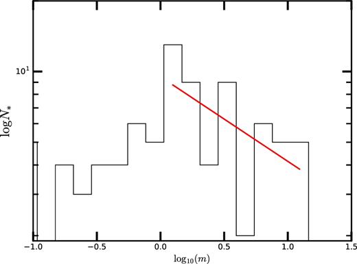
IMF for the ramses run with NJ = 32. The peak of the IMF is at 2 M⊙ and the high-mass slope is Γ = 1.36, where the Saltpeter slope is Γ = 2.35. The red line shows the least-squares fit to the mass function for M ≥ 1.0 M⊙. Our IMF varies with time with the peak mass moving to lower mass and the value of Γ increasing with time.
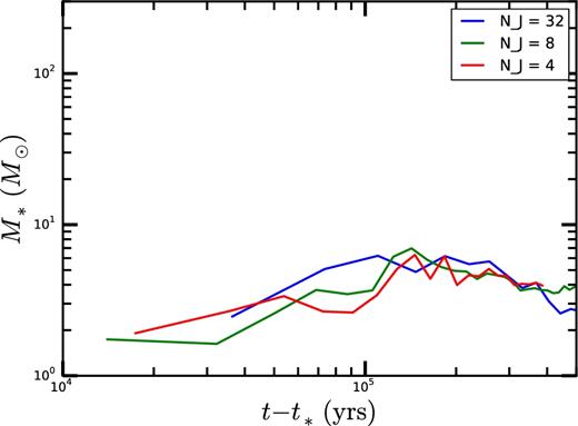
Average stellar mass as a function of time for the ramses run with NJ = 32 in green. Average stellar mass starts at ≈1 M⊙ increasing to ≈6 M⊙ and then decreasing as low-mass star formation begins. We also show the average stellar mass for NJ = 8 (blue) and 4 (red). This demonstrates that NJ = 4 runs are converged.
Fig. D2 shows the average stellar mass as a function of time. We see that the average mass is significantly higher than that of observed IMFs, where it is in the range of 0.3–1.0. In addition, we see that this average mass rises initially as the massive stars grow and then decreases as low-mass star formation kicks in.
APPENDIX E: CONVERGENCE WITH NJ
In this appendix, we examine how our results for the mass accretion rate depend on the resolution of the Jeans length, as quantified by NJ.
Fig. E1 shows the total mass in stars plotted as a function of time since the time t* at which the first star particle formed, for NJ = 4, 8, and 32. For the NJ = 32 run, the final value of the total stellar mass |$M_{\ast }\approx 240\,\text{M}_{\odot }$| (for NJ = 32) is about 1 per cent of the total gas mass in the box, while the final t − t* ≈ 0.6 Myr, about 15 per cent of the free-fall time 3.8 Myr for the mean density of the box. The green line shows the total stellar mass for NJ = 8, while the red line shows the same quantity for NJ = 4.
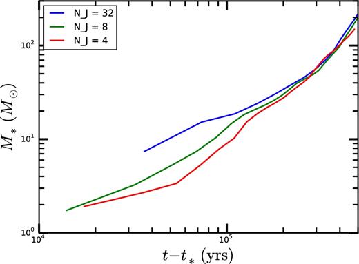
Plot of M*(t − t*) for ramses runs with NJ = 32 (blue), 8 (green), 4 (red). At the end of the NJ = 32 run, the total stellar mass was |$M_{\ast }\approx 240\,\text{M}_{\odot }$|.
The figure shows that for t − t* > 200 000 year, the stellar mass as a function of t − t* is converged to within 10 per cent and to even better accuracy at late times.
We have also done a convergence study for the average mass, see Fig. D2, showing that the mean stellar mass is converged for NJ = 4. This is consistent with the IMF being converged, albeit to a form that is not in good agreement with observations. We remind the reader that because of our use of an isothermal equation of state, we do not expect the IMF to match measured IMFs.
As a further convergence check, Fig. E2 shows the run of density as a function of radius for three different ramses simulations. The NJ = 32 (blue) run had three star particles at |$0.5\,\text{M}_{\odot }<M_{\ast }<3 \,\text{M}_{\odot }$|, while both the NJ = 8 (green line) run and the NJ = 4 (red line) had nine star particles. We see convergence for all radii larger than the disc radius, rd. This illustrates that the density approaches an attractor solution that is robust against the underlying numerical technique.
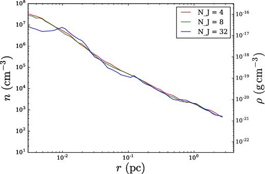
Plot of ρ(r) for ramses runs with NJ = 32 (blue), 8 (green), 4 (red). These are the averaged profiles of the density for star particles with |$0.5\,\text{M}_{\odot }\le M_{\ast }\le 3 \text{M}_{\odot }$|. Each simulation had ≈88 M⊙ worth of the gas in star particles. The density for r > rd is the same all three runs, showing that the NJ = 4 run is converged for r > rd.
