


Abstract
We present mass models of the Milky Way created to fit observational constraints and to be consistent with expectations from theoretical modelling. The method used to create these models is that demonstrated in our previous study, and we improve on those models by adding gas discs to the potential, considering the effects of allowing the inner slope of the halo density profile to vary, and including new observations of maser sources in the Milky Way amongst the new constraints. We provide a best-fitting model, as well as estimates of the properties of the Milky Way. Under the assumptions in our main model, we find that the Sun is R0 = 8.20 ± 0.09 kpc from the Galactic Centre, with the circular speed at the Sun being v0 = 232.8 ± 3.0 km s−1; and that the Galaxy has a total stellar mass of (54.3 ± 5.7) × 109 M⊙, a total virial mass of (1.30 ± 0.30) × 1012 M⊙ and a local dark-matter density of 0.40 ± 0.04 GeV cm−3, where the quoted uncertainties are statistical. These values are sensitive to our choice of priors and constraints. We investigate systematic uncertainties, which in some cases may be larger. For example, if we weaken our prior on R0, we find it to be 7.97 ± 0.15 kpc and that v0 = 226.8 ± 4.2 km s−1. We find that most of these properties, including the local dark-matter density, are remarkably insensitive to the assumed power-law density slope at the centre of the dark-matter halo. We find that it is unlikely that the local standard of rest differs significantly from that found under assumptions of axisymmetry. We have made code to compute the force from our potential, and to integrate orbits within it, publicly available.
1 INTRODUCTION
The field of Milky Way dynamics is reaching an incredibly exciting time, as the successful launch and operation of the European Space Agency's Gaia satellite (Gaia Collaboration 2016) mean that we will soon have access to proper motions and parallaxes for a billion stars. This represents an increase of four orders of magnitude over the number of stars with known parallaxes from Gaia's predecessor, Hipparcos (Perryman et al. 1997). This information will revolutionize how we understand our own Galaxy, and by extension, the Universe as a whole.
However, Gaia can only measure the present velocities of stars, not their accelerations due to the Galactic gravitational potential. These accelerations are far too small, of the order of cm s−1 yr−1. This means that the Galaxy's gravitational field can only be inferred, not measured. The stars seen by Gaia orbit in the potential of the Milky Way, and it is the nature of their orbits (best characterized by their actions; e.g. Binney & McMillan 2016) that are generally of real interest for understanding Galactic structure, rather than their exact positions and velocities at this moment. To determine the stars’ orbits, we need to know the underlying potential.
This paper follows a long tradition of authors who have produced mass models of the Milky Way, with the intention of synthesizing all of the knowledge about the components of the Milky Way into a coherent picture of the gravitational potential of the Galaxy. A famous early example was that of Schmidt (1956), with further examples being provided by Caldwell & Ostriker (1981), Dehnen & Binney (1998a, henceforth DB98), Klypin, Zhao & Somerville (2002) and the previous paper in this series (McMillan 2011, henceforth Paper I).
We return to this subject for three main reasons. First, because our knowledge of the Milky Way has increased substantially since Paper I was written, with new constraints that should be synthesized to produce a superior model. Secondly, Paper I did not include a component representing the Milky Way's cold gas. This gas forms a vertically thin component in the Galactic mid-plane, which deepens the potential well close to the plane, significantly affecting the dynamics of stars in the Solar neighbourhood. This means it is important to include this component. Thirdly, Gaia is due to release data in the very near future, which will dramatically increase our knowledge of the positions and velocities of stars in the Milky Way. It is therefore useful to have a model that reflects our current knowledge of the Milky Way's potential, to allow us to calculate the best estimates of the orbits of these stars (and their properties, such as the actions; Sanders & Binney 2016). It also provides a helpful estimate of the potential that can be refined by dynamical modelling (e.g. Bovy & Rix 2013; McMillan & Binney 2013; Piffl et al. 2014a).
To find the gravitational potential associated with a given mass model, we use the publicly licensed code galpot, which is described by DB98. We have made an edited version of this software available on GitHub, along with files giving the parameters of the best-fitting model potentials found in this study in a form that galpot can read. We also provide routines to integrate orbits in this potential.1 In Appendix A, we give examples of using this code.
In Section 2, we describe the components of our model of the Milky Way and some of the constraints we apply to them. In Section 3, we describe the kinematic data that our model has to fit, and Section 4 explains how we perform the model fits. Section 5 gives the properties of our main model and discusses some of its implications, and in Section 6 we explore alternative models. Finally, in Section 7 we compare our results to those of other authors (and discuss reasons that they may differ), before drawing conclusions in Section 8.
2 COMPONENTS OF THE MILKY WAY
We decompose the Milky Way into six axisymmetric components: bulge dark-matter halo, thin and thick stellar discs, and H i and molecular gas discs. This is similar to that used in Paper I, with the addition of the gas discs. We recap the main properties briefly and give details of the components that are new (or have different properties) in this model.
2.1 The bulge
The Galactic bulge has been known for some time to be a triaxial rotating bar with its long axis in the plane of the Galaxy (e.g. Binney, Gerhard & Spergel 1997). It is increasingly clear that it is a boxy (or ‘peanut shaped’) bulge (McWilliam & Zoccali 2010; Nataf et al. 2010; Ness et al. 2012, and others).
Our model is axisymmetric for ease of calculation. We must therefore accept that it cannot accurately represent the inner few kpc of the Galaxy, and we should not expect it to reproduce measurements taken from that part of the Galaxy. It is difficult to take constraints on our model from studies of the bulge as they naturally reflect its triaxial shape. Indeed, as noted by Portail et al. (2015), different studies of the bulge constrain the mass in different regions and use different definitions of what constitutes the bulge.
Our density profile is (as in Paper I) based on the parametric model fit by Bissantz & Gerhard (2002) to dereddened L-band COBE/DIRBE data (Spergel, Malhotra & Blitz 1996), and the mass-to-light ratio determined by Bissantz & Gerhard (2002) from a comparison between gas dynamics in models and those observed in the inner Galaxy. We note that the more recent (non-parametric) study of Portail et al. (2015) states that the total bulge mass that they find compares well with that of Bissantz & Gerhard (2002), when they consider the region R < 2.2 kpc. We have chosen not to directly apply the Portail et al. (2015) constraint on the total mass in the bulge to our model because it only describes the inner 2.2 kpc, while our bulge model has around 20 per cent of its mass outside that radius. We compare our result to the Portail et al. (2015) result in Section 7, and find reasonable agreement, which is as good as we can expect given the simplifications of our model.
2.2 The stellar discs
The Jurić et al. (2008) analysis of data from the Sloan Digital Sky Survey (SDSS; Abazajian et al. 2009) showed that the approximation to exponential profiles is a sensible one for the Milky Way, and produced estimates based on photometry for the scalelengths, scaleheights and relative densities of the two discs. As in Paper I, use these values as constraints. We hold the scaleheights of the discs fixed as zd, thin = 300 pc and zd, thick = 900 pc. In Paper I, we showed that our models are not significantly affected by the choice of scaleheights. We take the scalelengths for the thin and thick discs to be 2.6 ± 0.52 and 3.6 ± 0.72 kpc, respectively, and the local density normalization fd, ⊙ = ρthick(R⊙, z⊙)/ρthin(R⊙, z⊙) is taken to be 0.12 ± 0.012. For a discussion of the many available studies of these parameters, see the review of the properties of the Milky Way by Bland-Hawthorn & Gerhard (2016).
Recent studies such as those of Bensby et al. (2011), Bovy et al. (2012a) and Anders et al. (2014) have shown that when the ‘thick disc’ of the Galaxy is defined chemically (as comprising stars with high [α/Fe]), it clearly has a shorter scalelength than the ‘thin disc’ (comprised of stars with low [α/Fe]). Since the high [α/Fe] component also has a larger scaleheight than the low [α/Fe] population, this might appear to be in conflict with the Jurić et al. (2008) result, and with thick discs observed in external galaxies (e.g. Yoachim & Dalcanton 2006), where the thick disc has the longer scalelength. However, this is simply because there is a distinction between defining the thick disc chemically, and defining it morphologically, easily explained if the chemically defined discs are flared (e.g. Minchev et al. 2015). Since we are only interested here in the morphology of the discs (and therefore their potential), we can happily accept the Jurić et al. (2008) result and not concern ourselves with the chemical properties of the two components we label as separate stellar discs.
2.3 The gas discs
The models used in Paper I contained no component representing gas in the Milky Way. Simple dynamical arguments demonstrate that this is a mistake when the model is used to understand stellar dynamics in the Solar neighbourhood. Since the gas discs have a much smaller scaleheight than the stellar component near the Sun, its presence significantly deepens the potential well near the Sun, even if the total surface density remains unchanged. This deeper well means that stars that reach far from the Galactic plane have large velocities in the z direction when they pass near the Sun. The potential due to the gas disc is therefore necessary to make the number of stars with high vz in the Solar neighbourhood dynamically consistent with the observed density of stars far from the Galactic plane.
There is still a great deal of uncertainty over the large-scale distribution of gas in the Milky Way (see discussions by Lockman 2002 and Kalberla & Dedes 2008, henceforth KD08).3 Both the H i and molecular gas discs have ‘holes’ with little gas in the inner few kpc, and the H i disc is significantly more extended in R and has a greater scaleheight.
Our H i disc model is designed to resemble the distribution found by KD08, but with significant simplifications, made in order to greatly simplify the force calculation using galpot. The largest simplification is that we neglect the flaring of the gas disc, and instead keep a constant scaleheight |$z_{\rm H\,\small {I}}=85\,\mathrm{pc}$|, consistent with the half-width half-maximum distance of 150 pc at R0 given by KD08. We set the surface density to be 10 M⊙ pc−2 at a fiducial value of R0 = 8.33 kpc, consistent with the value given by KD08. It is worth noting that the KD08 value is the total surface density of all the gas associated with H i, i.e. not just the hydrogen (Kalberla private communication). This is not made clear in KD08, and this has led some authors to (mistakenly) add an ∼40 per cent correction for helium and metals (e.g. Hessman 2015). We set Rm, HI = 4 kpc and Rd, HI = 7 kpc, which produces a surface density that varies more smoothly than that of KD08 (which has a constant surface density for 4 kpc ≲ R ≲ 12.5 kpc and an exponential decline for R ≳ 12.5), but is broadly similar, and shares the property of having ∼21 per cent of the H i mass at R < R0. The total mass in the H i component (including helium and metals) is 1.1 × 10¹⁰ M⊙.
Our molecular gas disc is intended to resemble that described by Dame (1993) and Olling & Merrifield (2001) in terms of scaleheight and surface density at the Solar position, and the Galactocentric radius of the peak in the surface density. We give it a constant scaleheight |$z_{\rm H_2}=45\,\mathrm{pc}$|, consistent with the full width at half-maximum value of ∼160 pc at R0 given by Olling & Merrifield. The surface density at the fiducial radius R0 = 8.33 kpc is set as 2 M⊙ pc−2, with scalelength |$R_{\rm d,H_2}=1.5\,\mathrm{kpc}$| and |$R_{\rm m,H_2} = 12\,\mathrm{kpc}$|, which places the maximum surface density at R = 4 kpc. The total mass in the molecular gas component is 1.2 × 10⁹ M⊙.
The parameters of these two discs are given in Table 1. We show the corresponding surface density profiles of these two discs in Fig. 1.
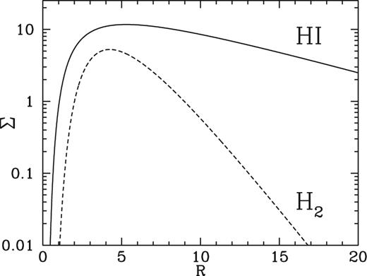
Surface densities, as a function of radius, of the two gas discs used in the model.
Parameters of the gas discs in the mass models. The first four columns enter the description of the disc in equation (4), from which one can derive the values in the final two columns.
| Disc | Rd | Rm | zd | Σ0 | Σ⊙ | M | ||
|---|---|---|---|---|---|---|---|---|
| ( kpc) | ( M⊙ pc−2) | ( M⊙) | ||||||
| H i | 7 | 4 | 0.085 | 53.1 | 10 | 1.1 × 10¹⁰ | ||
| H2 | 1.5 | 12 | 0.045 | 2180 | 2 | 1.2 × 10⁹ | ||
| Disc | Rd | Rm | zd | Σ0 | Σ⊙ | M | ||
|---|---|---|---|---|---|---|---|---|
| ( kpc) | ( M⊙ pc−2) | ( M⊙) | ||||||
| H i | 7 | 4 | 0.085 | 53.1 | 10 | 1.1 × 10¹⁰ | ||
| H2 | 1.5 | 12 | 0.045 | 2180 | 2 | 1.2 × 10⁹ | ||
2.4 The dark-matter halo
It is still unclear what effect the baryons in galaxies have on dark-matter profiles. The main influence will be at the centre, but whether, for Milky Way sized galaxies, this influence will be to steepen the inner density ‘cusp’ (corresponding to γ > 1 in equation 5) or to weaken it, producing more of a ‘core’ (γ < 1) is an active area of research (e.g. Duffy et al. 2010; Governato et al. 2012). In Section 6.1, we explore the effect of varying the assumed value of γ.
Haloes in dark-matter-only cosmological simulations tend to be significantly prolate, but with a great deal of variation in axis ratios (e.g. Allgood et al. 2006). It is recognized that, again, baryonic physics will play an important role– condensation of baryons to the centres of haloes is expected to make them rounder than dark-matter-only simulations would suggest (Debattista et al. 2008). The shape of the Milky Way's halo is still very much the subject of debate, with different efforts to fit models of the Sagittarius dwarf's orbit favouring conflicting halo shapes (see e.g. Law, Majewski & Johnston 2009). In this study, we will only consider spherically symmetric haloes.
Moster et al. (2013) assume an intrinsic scatter around this relationship of 0.15 in log 10M* and also give a ‘plausible range’ for all of the parameters in equation (7). It is not straightforward to convert a range of plausible parameters into an uncertainty in the typical stellar mass at a given Mv (which is what we require), especially as we do not know the correlations between the various parameters (e.g. are certain values of N only plausible for certain other values of M1?). Based on the ranges given, we can conservatively estimate that the uncertainty in the best-fitting value is ∼0.15 in log 10M* (i.e. similar to the intrinsic spread). Combining this uncertainty of the best-fitting value in quadrature with the expected scatter around the best-fitting value, we come to a total uncertainty in log 10M* of ±0.2 about the value given by equation (7).
Once the shape of a dark-matter halo profile has been chosen [e.g. the form of equation (5) and a value for γ], there are still typically two parameters required to describe it. In the case of equa-tion (5), these are the scale radius and density, but it is common for cosmologists to use instead the virial mass and the concentration cv. The concentration is given by cv = rv/r−2, where r−2 is the radius at which the derivative d log ρ/d log r = −2. In the case of the density profile in equation (5), r−2 = (2 − γ) rh.
Baryonic physics is likely to have an effect on the concentration, much as it does on the inner density profile. Duffy et al. (2010), who found increases in the inner density slope of dark-matter profiles from baryonic processes, found that the concentrations of the haloes were also altered. Some had higher concentrations and some lower, depending on the type of cooling or feedback used in the simulations. These changes were typically ∼20 per cent. Since we have no clear indication of what changes in cv we should expect as γ changes, and since the uncertainty in our constraint on cv is larger than the typical changes found by Duffy et al. (2010), we take equation (8) as our prior on cv even when we consider models with γ ≠ 1.
2.5 The Sun
There is still some uncertainty about the distance from the Sun to the Galactic Centre R0 (for a review, see Bland-Hawthorn & Gerhard 2016). Since the interpretation of all of the observational data considered in Section 3 depends on R0, we leave it as a free parameter in our models.
3 KINEMATIC DATA
3.1 Maser observations
A small but increasing number of Galactic maser sources have been targeted for extremely accurate astrometric measurements, with uncertainties of ∼ 10 μas, using very long baseline interferometry. This allows us to determine the full six-dimensional phase-space coordinates of these sources to high accuracy, as it provides parallaxes and proper motions, as well as line-of-sight velocities. Maser sources are associated with high-mass star forming regions (HMSFR) which are expected to be on near circular orbits. They have therefore been used by numerous authors to constrain the properties of the Milky Way (e.g. Bovy, Hogg & Rix 2009; Reid et al. 2009a; McMillan & Binney 2010; Bobylev & Bajkova 2013; Reid et al. 2014, Paper I).
In order to avoid using any data from HMSFRs likely to be strongly affected by the Galactic bar, we remove any sources that are likely to be at R < R0/2 for a fiducial value of R0 = 8.33 kpc. We perform this cut by insisting that there is no point within the 1σ error bars on parallax for a given object that would place it within this radial range. This reduces the number of HMSFRs used in the analysis to 93. We note that Chemin, Renaud & Soubiran (2015) emphasize that the assumption of a circular rotation curve is likely to provide false results for the Galactic gravitational potential in the inner ∼4 kpc because of the influence of the bar.
3.2 Other kinematic data
The other kinematic data we consider are the same as were used in Paper I. We summarize them here.
3.2.1 The Solar velocity
3.2.2 Terminal velocity curves
3.2.3 Vertical force
3.2.4 Mass within large radii
4 FITTING THE MODELS
In Paper I, we outlined a scheme to fit mass models of the Galaxy to the sort of constraints described above. We use the same techniques again here. They were also used by Piffl et al. (2014a) as constraints on dynamical models fit to Radial Velocity Experiment (RAVE) data (Kordopatis et al. 2013), though in that study only best-fitting models were found in each case, not the full pdf on all model parameters.
We have 15 free parameters: the scalelengths and density normalizations of the thin and thick discs (Rd, thin, Σ0, thin, Rd, thick, Σ0, thick); the density normalization– and thus mass– of the bulge (ρ0, b); the scale radius and density normalization of the cold dark matter halo (rh, ρ0, h); the solar radius (R0); the three components of |${\boldsymbol {v_{\odot}}}$|; the three components of |${\boldsymbol {v_{\rm SFR}}}$| and the typical random component of the HMSFR velocity Δv. We have direct priors on many of these parameters, or on quantities that can be directly derived from them, as described above.
Clearly, this is too large a parameter space to explore by brute force. We therefore use a Markov Chain Monte Carlo (MCMC) method, the Metropolis algorithm (Metropolis et al. 1953), to explore the pdf. This explores the full pdf, and the output chain is a fair sample of the pdf. As a test, we have also used the affine invariant MCMC sampler proposed by Goodman & Weare (2010), and packaged as emcee by Foreman-Mackey et al. (2013), to explore the pdf of some of our models, and found essentially identical results.
5 MAIN MODEL
Our ‘main’ model has an NFW halo (i.e. γ = 1 in equation 5). In Table 2, we give the expectation values and standard deviations, and median and ±1σ equivalent range, for the parameters of our model, and various derived quantities of interest. We define the ±1σ equivalent range as being between the 15.87 and 84.13 per cent points in the cumulative distribution (the percentage equivalents of the 1σ range in a Gaussian distribution). We include this because a few of our parameters have significantly non-Gaussian distributions, but in most cases we will quote the standard deviations of values.
Expectation values and uncertainties (upper rows), and median and ±1σ equivalent range (lower rows) for the free parameters of the mass model as described by equations (1), (3) and (5) (top), the peculiar velocity of the Sun and free parameters of the maser velocity pdf as described by equations (11) and (12) (middle) and derived properties of the mass model (bottom). Mb is the bulge mass, M* is the total stellar mass and ρh, ⊙ is the halo density at the Sun's position. Distances are quoted in units of kpc, velocity in km s−1, masses in 109 M⊙, surface densities in M⊙ pc−2, densities in M⊙ pc−3 and Kz, 1.1, ⊙ in units of (2πG) × M⊙ pc− 2. The local dark-matter density can also be written as 0.40 ± 0.04 GeV cm−3.
| Σ0, thin | Rd, thin | Σ0, thick | Rd, thick | ρ0, b | ρ0, h | rh | R0 | |
|---|---|---|---|---|---|---|---|---|
| Mean ± Std Dev | 886.7 ± 116.2 | 2.53 ± 0.14 | 156.7 ± 58.9 | 3.38 ± 0.54 | 97.3 ± 9.7 | 0.0106 ± 0.0053 | 19.0 ± 4.9 | 8.20 ± 0.09 |
| Median and range | |$887.0 _{- 115.0 }^{+ 116.6 }$| | |$2.53 _{- 0.14 }^{+ 0.15 }$| | |$148.7 _{- 53.2 }^{+ 73.1 }$| | |$3.29 _{- 0.45 }^{+ 0.63 }$| | |$97.3 _{- 9.8 }^{+ 9.7 }$| | |$0.0093 _{- 0.0034 }^{+ 0.0059 }$| | |$18.6 _{- 4.4 }^{+ 5.3 }$| | |$8.20 _{- 0.09 }^{+ 0.09 }$| |
| U⊙ | v⊙ | W⊙ | vR, SFR | vϕ, SFR | vz, SFR | Δv | ||
| Mean ± Std Dev | 8.6 ± 0.9 | 13.9 ± 1.0 | 7.1 ± 1.0 | −2.7 ± 1.4 | −1.1 ± 1.3 | −1.9 ± 1.4 | 6.8 ± 0.6 | |
| Median and range | |$8.6 _{- 0.9 }^{+ 0.9 }$| | |$13.9 _{- 1.0 }^{+ 1.0 }$| | |$7.1 _{- 1.0 }^{+ 1.0 }$| | |$-2.7 _{- 1.4 }^{+ 1.4 }$| | |$-1.1 _{- 1.3 }^{+ 1.3 }$| | |$-1.9 _{- 1.4 }^{+ 1.4 }$| | |$6.8 _{- 0.6 }^{+ 0.6 }$| | |
| v0 | Mb | M* | Mv | |$c_{{\rm v}^{\prime }}$| | Kz, 1.1, ⊙ | ρh, ⊙ | ||
| Mean ± Std Dev | 232.8 ± 3.0 | 9.13 ± 0.91 | 54.3 ± 5.7 | 1300 ± 300 | 16.4 ± 3.1 | 74.8 ± 4.9 | 0.0101 ± 0.0010 | |
| Median and range | |$232.8 _{- 3.0 }^{+ 3.0 }$| | |$9.13 _{- 0.92 }^{+ 0.91 }$| | |$54.3 _{- 5.8 }^{+ 5.6 }$| | |$1300 _{- 300 }^{+ 300 }$| | |$16.0 _{- 2.7 }^{+ 3.4 }$| | |$74.8 _{- 4.9 }^{+ 4.9 }$| | |$0.0101 _{- 0.0010 }^{+ 0.0010 }$| |
In Table 3, we give the parameters of our best-fitting model. Figs 3–5 show the marginalized pdfs for various properties of the models.
Parameters and properties of our best-fitting model.
| Parameter | Property | ||
|---|---|---|---|
| Σ0, thin | 896 M⊙ pc−2 | v0 | 233.1 km s−1 |
| Rd, thin | 2.50 kpc | Mb | 9.23 × 10⁹ M⊙ |
| Σ0, thick | 183 M⊙ pc−2 | M* | 5.43 × 10¹⁰ M⊙ |
| Rd, thick | 3.02 kpc | Mv | 1.37 × 10¹² M⊙ |
| ρ0, b | 98.4 M⊙ pc−3 | |$c_{{\rm v}^{\prime }}$| | 15.4 |
| ρ0, h | 0.00854 M⊙ pc−3 | Kz, 1.1, ⊙ | 73.9 × (2πG) M⊙ pc− 2 |
| rh | 19.6 kpc | ρh, ⊙ | 0.0101 M⊙ pc−3 |
| R0 | 8.21 kpc |
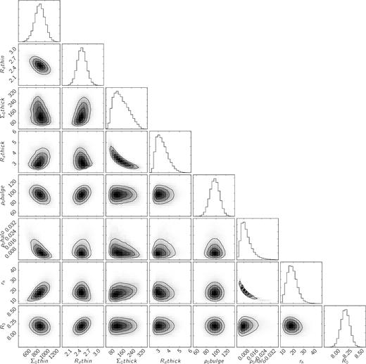
Two-dimensional pdf of the main parameters. The correlation coefficients are given in Table 4.
The strongest correlations or anticorrelations are typically, as in Paper I, between parameters that combine to define the properties (such as the total mass) of a component. ρ0, h and rh are very strongly anticorrelated, as are Σ0, thick and Rd, thick. This explains, for example, why the spread in ρ0, h is much larger than that in Mv. There are fairly strong correlations between Σ0, thin and most other parameters, and between R0 and Rd, thin. This is very similar to the correlations found in Paper I.
Fig. 3 shows the pdf for the scalelength of the thin disc along with the prior from Jurić et al. (2008). The peaks lie at nearly the same value of Rd, thin, but the range of plausible values we find is smaller than in the prior. This is noticeably different from the value of 3.00 ± 0.22 kpc found in Paper I. This is partially due to the new data we consider and partly due to the omission of a gas disc in Paper I. If we omit the gas discs from our models, we find thin-disc scalelengths of ∼2.8 kpc. The gas discs reduce the value of Rd, thin because the H i disc provides a component of the disc mass that has a longer scalelength than the stellar components. To compensate in the fit of the kinematic data, the scalelength of the stellar component decreases. This emphasizes the importance of modelling assumptions in finding the parameters, and therefore of including a component to represent the gas disc. In Section 6.4, we explore the consequences of changing the mass of the gas component in more detail.

Histogram of the pdf of the thin-disc scalelengths in our model (solid histogram) normalized over all other parameters, compared to the prior pdf described in Section 2.2 (dotted).
The pdfs of R0 and (v0 + V⊙)/R0, as shown in Fig. 4, both are displaced to slightly lower values than the priors (which, in the latter case, is the proper motion of Sgr A*). In the case of R0, this is ∼1σ lower than the value from the prior. The value of R0 is clearly pulled down by the need to fit the maser data (an effect that was not noticeable when using data from the 24 masers observed before Paper I). In experiments where we applied a weaker prior to R0 (8.33 ± 0.35 kpc, as in Paper I), the value of R0 found is even lower, at ∼8.0 kpc.
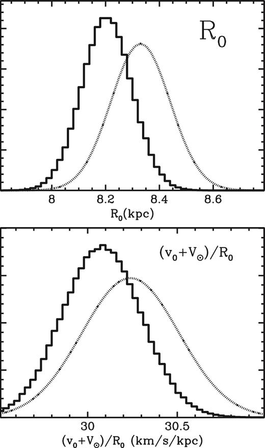
Histograms of the pdf of R0 (upper) and (v0 + V⊙)/R0 (lower) with the model output shown as a solid histogram, and the prior on each quantity shown as a dotted curve. In the lower panel, the prior shown is that associated with the proper motion of Sgr A*.
This lower value of R0 is the primary cause of our derived value of v0 being lower than in Paper I (where it was ∼239 km s−1). Our value of 232.8 km s−1 lies neatly between the ‘traditional’ value of 220 km s−1 and the values found by more recent studies which tend to be closer to ∼240 km s−1 (e.g. Schönrich 2012; Reid et al. 2014). It is rather close to the value found by Sharma et al. (2014) from RAVE data.
In Fig. 5, we show pdfs of the stellar mass and virial mass of our models (upper panels). The lower panels show how the halo concentration compares to our prior (typically slightly higher than expected, but well within the uncertainties), and how the stellar mass compares to our prior, given the virial mass (again, slightly higher than expected, but well within the range expected). These results are very similar to those found in Paper I.
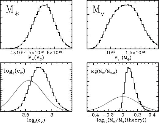
Histograms of the pdf total stellar mass (M*, upper left), virial mass (Mv, upper right), natural logarithm of the halo concentration (|$\log c_{v^{\prime }}$|, lower left) and the logarithm of the ratio of the stellar mass to that predicted by equation (7) given the virial mass (lower right). In the lower panels, the priors on the plotted properties are shown as dotted curves.
In Fig. 6, we show the pdf of values for M50, with a representation of the prior for comparison. The prior clearly provides an important upper bound. This is to be expected because no other data that we use as input are able to provide any useful constraint on the potential in the outer parts of the Galaxy. We observed the same behaviour in Paper I. It is clear that there are a range of values of M50 below MWE that provide acceptable models. If we remove the prior on M50, then the peak of our pdf in M50 is still found at ∼MWE, but the distribution is more symmetric about the peak.
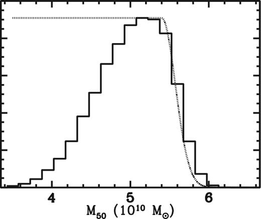
pdf of the mass contained within 50 kpc (M50, solid histogram). The dotted line illustrates the prior on M50. Since this prior is a constant for M50 < 5.4 × 10¹¹, we have artificially chosen to rescale this constant to the same value as the peak of the binned pdf in the interests of making comparison easier.
5.1 Maser velocities
The typical peculiar velocity associated with the maser sources is small, the largest being a velocity of 2.7 ± 1.3 km s−1 radially inwards. We find that the claimed lag in the rotational velocity is negligible: 1.1 ± 1.4 km s−1. This is in contrast to the lag that is claimed by Reid et al. (2014) using the same data, which was 5.0 ± 2.2 km s−1 when they use the Schönrich et al. (2010) value of |${\boldsymbol {v_{\odot}}}$| as a prior. There are three main differences between this study and Reid et al. (2014) that, together, are likely to have caused this difference. First, that our rotation curves come from our mass model rather than any of the assumed forms used by Reid et al. Secondly, that we marginalize over all possible distances to the objects rather than approximating that the quoted parallax gives the true distance. We note that in some cases (e.g. G023.65-00.12 and G029.95-00.01) this means that sources labelled as outliers by Reid et al. (2014) prove to be well fitted by our models within the parallax uncertainties but not at the quoted parallax. Thirdly, we use an outlier model to take account of objects which have significantly non-circular motions rather than removing them from the analysis entirely. These results are not significantly altered if we increase the outlier fraction fout to 0.1.
The intrinsic spread of the HMSFR velocities around a circular orbit (ignoring the outliers) is 6.8 ± 0.6 km s−1, which is comparable to the values found by McMillan & Binney (2010) and the value assumed in Paper I. It is a little larger than the value of 5 km s−1 assumed by Reid et al. (2014).
5.2 Solar position and velocity
The value of R0 we find is 8.20 ± 0.09 kpc, which is ∼1σ below the value taken as a prior (equation 9). It is also a little lower than the value found in Paper I of 8.29 ± 0.16 kpc, by Schönrich (2012) of 8.27 ± 0.29 kpc or by Reid et al. (2014) of 8.34 ± 0.16 kpc. It is still consistent with these values, and with the distance to the Galactic Centre found from the parallax to Sgr B2 (|$7.9^{+0.8}_{-0.7}\,\mathrm{kpc}$|; Reid et al. 2009b). It is very close to the distance (and uncertainty) found from a compilation of literature values by Bland-Hawthorn & Gerhard (2016). Since the prior placed on v0/R0 by the proper motion of Sgr A* is still closely followed, we therefore find a somewhat lower value of v0 than Paper I, 232.6 ± 3.0 km s−1. This re-emphasizes the point made by McMillan & Binney (2010) that estimates of v0 are typically highly dependent on R0, so it is dangerous to treat R0 as known and fixed. In Fig. 7, we plot the distribution of values of R0, v0 and V⊙ from our MCMC chain. The clearest feature is the strong correlation between R0 and v0.
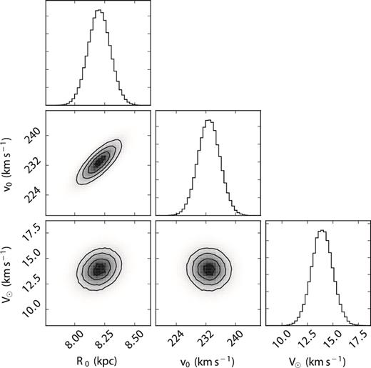
Two-dimensional histograms showing the distribution of values found in the MCMC simulation for R0, v0 and V⊙. The dominant feature is the correlation between R0 and v0.
The differences between these values of R0 and v0 and those found in Paper I are at around the 1σ level (less when both uncertainties are taken into account). These can be attributed to the changed modelling assumptions (including the addition of a gas disc and allowing |${\boldsymbol {v_{\odot}}}$| to vary) as well as the additional data.
The peculiar velocity |${\boldsymbol {v_{\odot}}}$| that we find differs somewhat from our prior taken from Schönrich et al. (2010), though only at the 1–2σ level. Our results suggest that the value of U⊙ may be a little smaller than suggested by Schönrich et al., and V⊙ may be a little larger.
The values of the components of |${\boldsymbol {v_{\odot }}}$| are correlated with the components of the typical peculiar motion associated with the maser sources |${\boldsymbol {v_{\rm SFR}}}$|. Table 5 shows the correlation matrix of the components of |${\boldsymbol {v_{\odot }}}$| with the components of |${\boldsymbol {v_{\rm SFR}}}$|.
The strong correlations that Table 5 show have been seen in previous studies (Reid et al. 2009a; McMillan & Binney 2010) and can be easily understood: consider the positions of the HMSFRs in Galactocentric polar coordinates (R, ϕ, z), where ϕ⊙ = 0. Any HMSFR at ϕ = 0 will have no change in expected heliocentric velocity if both |${\boldsymbol {v_{\odot }}}$| and |${\boldsymbol {v_{\rm SFR}}}$| change by the same amount. For ϕ ≠ 0, there will be some difference, increasing as ϕ goes further from 0. The majority of the observed sources are at ϕ relatively close to zero, which causes this correlation.
If we remove the Schönrich et al. (2010) constraint on the Sun's peculiar velocity, then the MCMC chain covers a broad range of values for the Sun's peculiar motion (especially V⊙), with the peculiar motion of the HMSFRs adjusting in exactly the way one would expect– if V⊙ increases by 15 km s−1, vSFR, ϕ must increase by ∼15 km s−1 to keep roughly the same relative motion. This means that numerical experiments without the Schönrich et al. (2010) prior (or something like it) are not useful for constraining the parameters. However, they do give us an insight into the implications of alternative estimates of |${\boldsymbol {v_{\odot }}}$| in the literature.
Schönrich (2012) suggested that Schönrich et al. (2010) may have underestimated the value of U⊙ and that it may be ∼14 km s−1. This would imply that the HMSFRs have a typical velocity radially inwards of ∼6 km s−1.
In a study of the kinematics of stars from a large range of Galactocentric radii observed by APOGEE (Wilson et al. 2010), Bovy et al. (2012b) found V⊙ = 26 ± 3 km s−1. They suggested that this could be consistent with local measurements (based on stars observed in the Solar neighbourhood) like that of Schönrich et al. (2010) if there was an offset between what they called the rotational standard of rest (RSR), which is the circular velocity at R0 in an axisymmetric approximation of the true potential (i.e. what we find in this study), and the velocity of a closed orbit, and therefore a theoretical 0 km s−1 dispersion population, in the Solar neighbourhood (which is what is found by local measurements like that of Schönrich et al. 2010). This would reflect large-scale non-axisymmetry of the potential. From our results, we can infer that this would require that a typical HMSFR leads circular rotation by ∼11 km s−1.
McMillan & Binney (2010) argued that large departures from circular rotation (larger than ∼7 km s−1) were implausible based on the known perturbations in the gas velocities due to non-axisymmetry in the potential and the low-velocity dispersion of the youngest stars observed in the Solar neighbourhood. These arguments still hold and suggest that both the Schönrich (2012) and Bovy et al. (2012b) results should be treated with some scepticism. It is worth noting that the results found by Bovy et al. (2012b) included a radial velocity dispersion that is nearly constant (or even increasing) with radius, where there are good physical reasons to expect it to fall with increasing radius, as well as observational evidence (Lewis & Freeman 1989). Sharma et al. (2014) noted that the use of Gaussian models of the kind used by Bovy et al. (2012b) can lead to this behaviour in the model velocity dispersion where other models do not because the Gaussian model is unable to properly represent the skewness of the vϕ distribution. This effect on velocity dispersion tends to increase the model value for V⊙ because of the effect on asymmetric drift. This may explain why the Bovy et al. (2012b) result differs so significantly from that found here or in the Solar neighbourhood studies. It is worth noting that Bovy et al. (2015) found a similar result to that of Bovy et al. (2012b) using a different technique to analyse the kinematics of red clump stars observed in the mid-plane of the Milky Way. They minimized the ‘large-scale power’ in the velocity field, having subtracted an axisymmetric velocity field. The axisymmetric velocity field subtracted was that found by Bovy et al. (2012b), but they did also experiment with a velocity distribution that had a velocity dispersion that fell with radius, finding similar results. It is not as obvious why the results of this study might differ so substantially from our results.
We have investigated whether the difference between this result and that of Bovy et al. (2012b) is dependent on data from the maser sources closest to the Sun. These observations have the smallest relative uncertainty, so they might be expected to carry great statistical weight. These closer observations would also suffer a very similar offset between the RSR and the velocity of closed orbits (the latter being what we expect the HMSFRs to follow, to a reasonable approximation). To check this, we have fitted our models to data sets that only include masers with quoted parallaxes ϖobs < 0.5 mas (i.e. quoted distances more than 2 kpc from the Sun, leaving only 62 masers). We find very similar results for the values of V⊙ and vSFR, ϕ– if anything the derived lag of the masers sources slightly increases to ∼2.5 km s−1 in the latter case.
As a final test, we fix vSFR = 0 and can then remove the Schönrich et al. (2010) prior on v⊙. In this case, again using only the 62 masers with ϖobs < 0.5 mas, we derive almost identical results for V⊙ (13.9 ± 1.0 km s−1) and R0 (8.21 ± 0.10 kpc). v0 increases by slightly over 1 to 234.4 ± 3.1 km s−1, and the spread in SFR velocities, Δv, increases slightly to 8.1 ± 0.9 km s−1. We conclude that our results regarding V⊙ are independent of the observations of masers in the vicinity of the Sun.
In Fig. 8, we give the distribution of maser sources in Galactocentric radius and the offset of their azimuthal velocity from that of a circular orbit in our best-fitting potential. It is clear that the sources sample a large range of radii, reaching far from the Solar neighbourhood.

Positions of the maser sources in Galactocentric radius, plotted against offset from circular velocity in the best potential. Error bars are found from a Monte Carlo sample within the uncertainties on the observations. The points in red are those where the quoted parallax is ϖ < 0.5, which are excluded from some experiments in Section 5.2.
6 ALTERNATIVE MODELS
6.1 Varying inner halo density profile
We have explored the effect of varying the inner slope of the dark-matter density profile (γ in equation 5). The density of the dark-matter halo goes as r−γ at r ≪ rh. This is a simple approach to exploring the question of whether the Milky Way's dark-matter halo is cusped (like the NFW profile) or not. As noted in Section 2.4, there are good reasons to believe that the halo profile has been changed from that expected in pure dark-matter simulations because baryonic processes will inevitably have had an effect. In reality there is no obvious reason for any effect that might have altered the dark-matter profile– be they baryonic processes or due to the unexpected nature of the dark-matter particle– to occur on the same physical scale as the halo's scale radius rh. The true density profile may be poorly characterized by a two-power-law equation like equa-tion (5). None the less, this numerical experiment does provide us with useful insights.
If we set γ to be a free parameter (with a flat prior), we find γ = 0.79 ± 0.32. This is a rather weak constraint, which is not too surprising since determining the value of γ depends sensitively on the details of the inner Galaxy (where we have the worst constraints) and to some extent on the outer Galaxy (where our constraints are also limited).
Perhaps more remarkable is the fact that the derived properties and uncertainties of these models are extremely similar to those found when we fix γ = 1. The thin-disc scalelength Rd, thin = 2.51 ± 0.15 kpc, which differs from that found where γ = 1 by only ∼20 pc (with ∼10 pc greater uncertainty). The derived value of R0 agrees to within 10 pc and the various derived velocities (v0 and the peculiar velocities of the Sun and maser sources) agree to within 0.2 km s−1. The derived total stellar mass is 56.6 ± 6.2 × 10⁹ M⊙, which is slightly higher than the value found with γ = 1, but well within the quoted uncertainty. The total virial mass is identical to the quoted precision.
The local dark-matter density is barely affected by setting γ free, with the local density 0.0099 ± 0.0009 M⊙ pc−3 (an ∼1 per cent change in the expectation value for the density, compared to a ∼10 per cent statistical uncertainty). This is rather surprising as one might expect the local dark-matter density to depend rather sensitively on the dark-matter density profile for r < rh. This merits some further examination. We have therefore investigated models with γ set at fixed values in the range 0 ≤ γ ≤ 1.5.
In Fig. 9, we show the expectation values and uncertainties of the local dark-matter density as a function of γ. We see that the change in expectation value of ρh, ⊙ is very small– it decreases by a few per cent as we go from a completely cored profile (γ = 0) to a very steeply cusped one. Indeed most of the properties we measure of the mass models (including v0) are only very slightly affected by the change of γ. Clearly what we have is a tight constraint on the local properties of the Milky Way rather than at any other point in the Galaxy. If the constraint on the dark-matter density was, instead, tightest at a radius ∼1 kpc less than R0, that would correspond to a 20 per cent change in ρh, ⊙ as we go from γ = 0 to γ = 1.5.
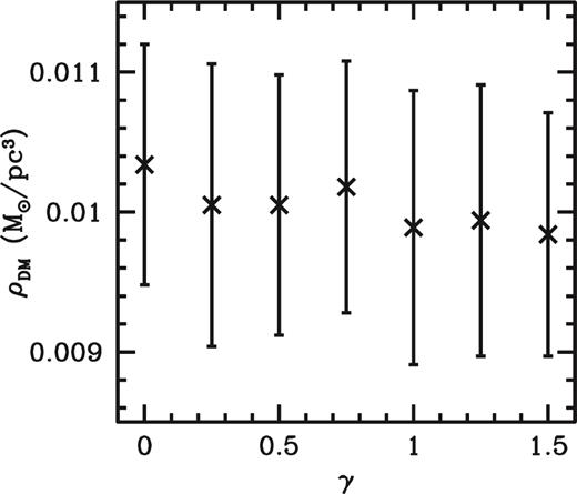
Local dark-matter density determined from models with differing inner density slopes for the dark-matter component (ρ∝r−γ for r ≪ rh). The trend is for slightly lower dark-matter density values for steeper inner density slopes, but the trend is much smaller than the individual error bars.
In Fig. 10, we show the properties of the models which do significantly change with varying γ. As γ increases, the halo becomes more centrally concentrated so the scalelength of the disc increases, making the disc less centrally concentrated, to compensate and leave the rotation curve essentially the same. The total disc mass decreases, for a similar reason. Meanwhile the halo scale radius decreases when γ decreases, to the point where rh < R0 for γ = 0. This has the effect that the slope of the halo density profile d log ρ/d log r is always ∼−1.5 at R0. The knock-on effect is that the virial mass of the halo increases with increasing γ.
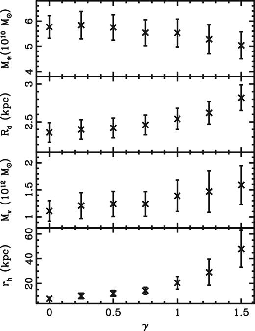
Properties of the model that strongly vary with inner density slope of the dark-matter component (ρ∝r−γ for r ≪ rh). The top two properties are for the stellar component– the total stellar mass M* and the thin-disc scalelength Rd, while the lower ones are for the whole Galaxy (the virial mass, Mv) and the dark-matter component only (scale radius rh).
6.2 Perturbing the disc
We now investigate whether small perturbations to the assumed exponential density profile (of the order of those expected due to spiral arms) have any significant effect on these results. If this is the case, it would imply that our assumed constraint on the density profile of the stellar discs was too strict. We do not include any non-axisymmetric component to the potential.
Results for models with these perturbations are shown in Table 6. Introducing this perturbation has almost no effect on the derived values of R0 or v0. It alters the derived scalelength of the thin disc by much less than 10 per cent, which is well within what one would naively expect. The derived stellar mass does change by ∼10 per cent (of a similar order to the derived statistical uncertainty), while the virial mass barely changes. The derived local dark-matter density is also affected by the perturbation (surprisingly, more than by any change in γ we considered), but this is still somewhat smaller than the statistical uncertainty.
DB98 used a similar form of perturbation to that given in equation (20), but had a rather longer scalelength for the perturbation, which was of the form εcos R/Rd (i.e. without the factor of π). They noted that this produced large changes to the rotation curve in the outer parts of the Milky Way. This perturbation goes from peak to trough over a distance of |$\pi \times R_\mathrm{d}\sim R_0$|. Its main effect is therefore to either increase or decrease the effective scalelength of the disc over the radial range that contains most of its mass. Since DB98 held the scalelength of the disc fixed for each model (and showed that varying it has important knock-on effects on the whole model), we suspect that the effect they describe is primarily due to the change in the effective scalelength rather than illustrative of an overconfidence introduced by assuming an exponential surface density profile. In our study, we have not found that introducing a perturbation of this form affects the results at large radii (illustrated by the virial mass being nearly unchanged in models with ε = ±0.1).
In his master's thesis, Zigmanovic (2016) found that the inclusion of a non-axisymmetric element to the velocity field for the maser sources and terminal velocity curve (to represent the effect of spiral structure) had a rather small impact on the parameters of a simple mass model of the Galaxy. It altered the derived local dark-matter density by a couple of per cent and had a similar effect on the mass contained within 50 kpc. While the effect of non-axisymmetric structure is clearly important for some studies of the potential of the Milky Way even outside the bulge (see e.g. Garbari et al. 2012), for our purposes here it is reasonable to ignore it.
6.3 An uncertain bulge
The prior that we take for the bulge is relaxed compared to the quoted uncertainty from Bissantz & Gerhard (2002), but as they make prior assumptions, it could be argued that this is a narrow range of possibilities. Portail et al. (2015) found a wider range of stellar masses within the region they studied (though the total mass was found with a very small uncertainty, sec Section 7). We have therefore investigated the effects of weakening our bulge prior such that it had an uncertainty of ±30 per cent on mass.
As we have noted before, the maser data and terminal velocity curve do not provide much of a constraint on the details of the bulge region because we have excluded these regions to avoid false conclusions caused by our assumption of axisymmetry. This means that weakening our bulge prior ensures that we will find a far greater range of possible bulge masses. In Fig. 11, we show the derived pdfs of the bulge mass for both the original prior (10 per cent uncertainty) and the weakened prior (30 per cent). In the latter case, the mass we find is (7.83 ± 2.30) × 109 M⊙. This mean value is lower than the value used as a prior (suggesting that other data favour a slightly lower mass bulge), but the spread of values comfortably includes the values associated with the tighter prior.
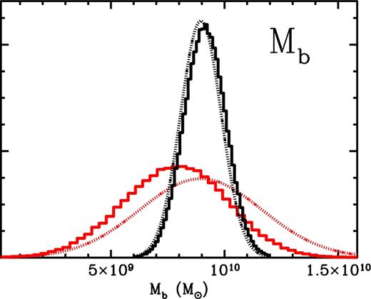
pdf of bulge mass for our normal (black) and relaxed (red) priors on bulge mass (10 and 30 per cent uncertainty, respectively). In both cases, the prior is shown as a dotted line and the derived pdf as a solid histogram. The derived pdf is, in both cases, reasonably close to the prior, indicating that the additional data do not provide significant constraints on the bulge.
The properties of the Galaxy models found with this weak prior are shown in Table 6. Almost all of the properties are essentially unchanged (as one would hope), but the scale radius of the disc is decreased from the main model value by ∼0.07 kpc (compared to an uncertainty of 0.16 kpc, up from 0.14 kpc in the main model). This is related to the lower average bulge mass– we can see in Table 4 or Fig. 2 that the two parameters are correlated.
| Σ0, thin | Rd, thin | Σ0, thick | Rd, thick | ρ0, b | ρ0, h | rh | R0 | |
|---|---|---|---|---|---|---|---|---|
| Σ0, thin | 1 | |||||||
| Rd, thin | −0.49 | 1 | ||||||
| Σ0, thick | −0.13 | 0.27 | 1 | |||||
| Rd, thick | 0.23 | −0.05 | −0.84 | 1 | ||||
| ρ0, b | −0.43 | 0.30 | −0.12 | 0.09 | 1 | |||
| ρ0, h | −0.61 | 0.02 | −0.42 | 0.25 | 0.04 | 1 | ||
| rh | 0.58 | −0.04 | 0.43 | −0.25 | −0.06 | −0.90 | 1 | |
| R0 | −0.14 | 0.38 | −0.01 | 0.10 | −0.02 | 0.14 | −0.11 | 1 |
Correlation matrix for the components of the peculiar motion of the Sun and the typical peculiar motion of the HMSFRs. The values given are, for example, corr(U⊙, vSFR, R) (equation 19). The strongest correlations are between components that, were the HMSFRs at the Sun's position, would have identical effects on the expected heliocentric velocity of the HMSFRs. Because of the sign conventions of the U⊙, V⊙andW⊙ system, corr(U⊙, vSFR, R) is negative (because they correspond to motions in opposite directions), while corr(V⊙, vSFR, ϕ) and corr(W⊙, vSFR, z) are positive (because they correspond to motion in the same direction).
| U⊙ | V⊙ | W⊙ | |
|---|---|---|---|
| vSFR, R | −0.57 | 0.00 | −0.03 |
| vSFR, ϕ | 0.12 | 0.69 | −0.03 |
| vSFR, z | 0.02 | −0.03 | 0.72 |
| U⊙ | V⊙ | W⊙ | |
|---|---|---|---|
| vSFR, R | −0.57 | 0.00 | −0.03 |
| vSFR, ϕ | 0.12 | 0.69 | −0.03 |
| vSFR, z | 0.02 | −0.03 | 0.72 |
We conclude that even if we substantially weaken the prior on our bulge component, the properties found for the rest of the Galaxy are not substantially affected.
6.4 Altered gas discs
The gas content of the Milky Way remains deeply uncertain, as discussed in Section 2.3. The gas disc models used (as described in Table 1) are efforts in good faith to capture the current understanding in a convenient form, but we have not attempted to fit them to the data, because we do not have the statistical leverage to do so. This does, however, introduce a systematic uncertainty that we have not accounted for.
In an effort to get some idea of how important this uncertainty is, we have investigated the effect of increasing or decreasing the total mass of the gas discs by 30 per cent (i.e. ∼± 3.5 × 10⁹ M⊙). This is approximately the level of spread seen when comparing different investigations of the H i disc (see e.g. KD08), which is the main component. We achieve this by simply changing the density at any point by the quoted factor (i.e. changing Σ0 in equation 4).
The results are given in Table 6, and the consequences are relatively minor. If we decrease the gas mass, the disc scalelength increases for the same reasons discussed in Section 5, and when we increase the gas mass, the disc scalelength decreases. There is a related effect that the total stellar mass increases when the gas mass increases (and they also decrease together), but by less than the change in gas mass (or the quoted uncertainties).
Properties of alternate mass models from our main models (we also include results from our main models for ease of comparison). These models are described in detail in Section 6. The properties shown are those that we consider most relevant to our discussion.
| Difference from | Rd, thin | R0 | v0 | ρh, ⊙ | rh | M* | Mv |
|---|---|---|---|---|---|---|---|
| main model | ( kpc) | ( kpc) | ( km s−1) | ( M⊙ pc−3) | ( kpc) | (109 M⊙) | (1012 M⊙) |
| Main model: γ = 1.00 | 2.53 ± 0.14 | 8.20 ± 0.09 | 232.8 ± 3.0 | 0.0101 ± 0.0010 | |$18.6 _{- 4.4 }^{+ 5.3 }$| | 54.3 ± 5.7 | 1.32 ± 0.29 |
| γ free (γ = 0.79 ± 0.32) | 2.51 ± 0.15 | 8.20 ± 0.09 | 232.5 ± 3.0 | 0.0098 ± 0.0009 | |$15.4 _{- 3.8 }^{+ 8.0 }$| | 56.6 ± 6.2 | 1.34 ± 0.28 |
| γ = 0 | 2.36 ± 0.13 | 8.21 ± 0.10 | 233.2 ± 3.0 | 0.0103 ± 0.0009 | |$7.7 _{- 0.9 }^{+ 1.4 }$| | 57.7 ± 4.5 | 1.11 ± 0.19 |
| γ = 0.25 | 2.40 ± 0.13 | 8.21 ± 0.10 | 232.9 ± 3.1 | 0.0100 ± 0.0010 | |$9.6 _{- 1.8 }^{+ 2.6 }$| | 58.4 ± 5.4 | 1.21 ± 0.24 |
| γ = 0.5 | 2.42 ± 0.13 | 8.20 ± 0.09 | 232.7 ± 3.0 | 0.0101 ± 0.0009 | |$11.7 _{- 1.9 }^{+ 2.6 }$| | 57.5 ± 5.1 | 1.24 ± 0.23 |
| γ = 0.75 | 2.46 ± 0.13 | 8.21 ± 0.09 | 232.9 ± 3.0 | 0.0102 ± 0.0009 | |$13.8 _{- 2.5 }^{+ 3.1 }$| | 55.4 ± 5.1 | 1.24 ± 0.23 |
| γ = 1.25 | 2.62 ± 0.15 | 8.20 ± 0.09 | 232.4 ± 3.0 | 0.0099 ± 0.0010 | |$27.2 _{- 7.2 }^{+ 9.5 }$| | 52.8 ± 5.8 | 1.47 ± 0.38 |
| γ = 1.5 | 2.82 ± 0.17 | 8.19 ± 0.09 | 232.4 ± 2.8 | 0.0098 ± 0.0009 | |$46.1 _{- 11.7 }^{+ 13.8 }$| | 50.4 ± 5.3 | 1.59 ± 0.36 |
| ε = −0.1 | 2.45 ± 0.13 | 8.19 ± 0.09 | 232.2 ± 2.9 | 0.0104 ± 0.0009 | |$19.0 _{- 3.5 }^{+ 4.1 }$| | 52.1 ± 4.9 | 1.39 ± 0.23 |
| ε = +0.1 | 2.61 ± 0.13 | 8.22 ± 0.09 | 233.3 ± 3.0 | 0.0093 ± 0.0010 | |$20.8 _{- 4.8 }^{+ 7.0 }$| | 59.4 ± 6.2 | 1.41 ± 0.37 |
| Weak bulge prior | 2.46 ± 0.16 | 8.20 ± 0.09 | 232.7 ± 3.0 | 0.0101 ± 0.0009 | |$18.8 _{- 3.8 }^{+ 5.1 }$| | 54.3 ± 5.3 | 1.35 ± 0.27 |
| Weak R0 prior | 2.38 ± 0.15 | 7.97 ± 0.15 | 226.8 ± 4.2 | 0.0098 ± 0.0010 | |$20.8 _{- 5.5 }^{+ 6.8 }$| | 52.0 ± 5.5 | 1.39 ± 0.35 |
| Gas discs ρ × 0.7 | 2.57 ± 0.14 | 8.20 ± 0.09 | 232.6 ± 2.9 | 0.0100 ± 0.0009 | |$19.9 _{- 4.2 }^{+ 4.9 }$| | 53.8 ± 5.4 | 1.39 ± 0.27 |
| Gas disc ρ × 1.3 | 2.45 ± 0.14 | 8.20 ± 0.09 | 232.6 ± 3.0 | 0.0100 ± 0.0009 | |$18.9 _{- 4.3 }^{+ 5.4 }$| | 57.1 ± 5.4 | 1.34 ± 0.28 |
6.5 Weaker R0 prior
The prior that we take on the distance to the Galactic Centre from Chatzopoulos et al. (2015) is derived from observations of objects near the Galactic Centre itself (the nuclear stellar cluster, and stars directly orbiting Sgr A*). These provide rather more direct estimates of this distance than techniques like those used in this study, which rely on the Galactic Centre being the centre of (circular) rotation for the Galaxy at large. That is why we have taken the (relatively narrow) prior from Chatzopoulos et al. (2015) despite the evidence that the maser observations drive us towards lower values of R0 (at 1σ below our prior).
None the less, we also consider the case with a weaker prior on R0, specifically the prior that we took in Paper I, which is simply derived from the measurements of the orbits of stars around Sgr A* by Gillessen et al. (2009) and is R0 = 8.33 ± 0.35 kpc. The results are shown in Table 6 and show significant differences from the results with the more restrictive prior. The thin disc scalelength decreases to 2.38 ± 0.15 kpc, which is roughly 1σ below the value for our main model, while R0 and v0 decrease more substantially to 7.97 ± 0.15 kpc and 226.8 ± 4.2 km s−1, respectively. The other main properties of the Galaxy are effected by less than the quoted uncertainties.
This serves to emphasize the importance of constraints on R0 when it comes to determining the circular velocity of the Milky Way. Because the Chatzopoulos et al. (2015) study provides constraints based on well-understood observations near the Galactic Centre, we chose to retain this prior when constructing our main models, but the tension between the value of R0 they derive and the value that the rest of our constraints drive us towards is worthy of further study.
7 COMPARISON TO OTHER STUDIES
Recent reviews by Bland-Hawthorn & Gerhard (2016) and Read (2014) provide excellent summaries of the literature related to the topics discussed in this paper. From an analysis of literature values of R0, Bland-Hawthorn & Gerhard (2016) adopt a best estimate of 8.20 ± 0.1 kpc, very much in keeping with the value found here. We note with interest, however, that a more recent analysis of the astrometry of faint stars orbiting Sgr A*, combining two different types of imaging over a time baseline of two decades, finds a lower value of R0 = 7.86 ± 0.14 ± 0.04 kpc (statistical and systematic uncertainties, respectively; Boehle et al. 2016). This is more similar to the results we find with a weaker prior and suggests that the value of R0 is still not fully settled.
Bland-Hawthorn & Gerhard (2016) also discuss the literature regarding the disc scalelengths, noting that estimates range from 1.8 to 6.0 kpc. They conclude from the 15 ‘main papers’ on the topic (it is not explicitly stated which papers these are) that the best estimate for the thin-disc scalelength is 2.6 ± 0.5 kpc, very similar to the value from Jurić et al. (2008) that we take as a prior. Our study provides a rather tighter constraint on this value, but we note that it also demonstrates that estimates of this value that are based on dynamics strongly depend on assumptions made regarding the other components of the Galaxy, such as the mass and scalelengths of the gas discs, and the density profile of the dark-matter halo.
Read (2014) gives a compilation of estimates of the local dark-matter density (his fig. 2 and table 4). The value we find (0.0100 ± 0.0010 M⊙ pc−3) is larger than many of the local measures in the compilation (though not all, e.g. Garbari et al. 2012, when no strong prior on the baryonic component is invoked). It is quite typical of values found when looking at the global structure of the Galactic potential (and assuming spherical symmetry, see Section 7.3), including Paper I, Catena & Ullio (2010) and Nesti & Salucci (2013).
Portail et al. (2015) used made-to-measure modelling to determine the mass within a box around the Galactic Centre of a volume ±2.2 ± 1.4 ± 1.2 kpc, determining that it is 1.84 ± 0.07 × 10¹⁰ M⊙ [and the closely related study by Portail et al. (2016) found a very similar value– (1.85 ± 0.05) × 1010 M⊙]. They note the difficulty of comparing different studies of the bulge because different studies probe different regions. They point out that Bissantz, Englmaier & Gerhard (2003) determined the circular velocity at 2.2 kpc to be 190 km s−1 and equate this (under the assumption of spherical symmetry) to a mass of 1.85 × 10¹⁰ M⊙. We find a circular velocity at 2.2 kpc of (198 ± 9) km s−1, which would correspond (again, assuming spherical symmetry) to a mass of ∼(2.01 ± 0.17) × 1010 M⊙. Our result is clearly comparable to these other studies, and given that the Portail et al. (2015) study looks at only a part of this region (though certainly the densest part, and it also includes a small volume outside a spherical shell of radius 2.2 kpc), it is reassuring that our result corresponds to a slightly higher mass than theirs. Again, we must emphasize that since our study is axisymmetric, it cannot accurately describe the bulge region, but the reasonable agreement between our study and that of Portail et al. (2015) is a useful sanity check.
7.1 The outer galaxy
Watkins, Evans & An (2010) used a sample of 26 satellite galaxies (including six with proper motions) to find the mass of the Milky Way within 300 kpc and found that the answer depended sensitively on the assumed velocity anisotropy of the satellites, with a mass estimate that was (1.4 ± 0.3) × 1012 M⊙ assuming isotropic velocities, but which could plausibly lie anywhere between 1.2 and 2.7 × 10¹² M⊙ when anisotropy is taken into account. Our estimate, which is (1.6 ± 0.3) × 1012 M⊙, fits comfortably in this range.
Deason et al. (2012) and Xue et al. (2008) used samples of blue horizontal branch stars to determine the mass contained within 50 and 60 kpc, respectively. In the latter case, cosmological simulations were used to provide a prior on the velocity anisotropy of the population. Fermani & Schönrich (2013) raise important concerns regarding the selection of stars for these studies.7 The cuts in log g and g-band magnitude used by Deason et al. (2012) lead to a very high risk of contamination by disc stars (Fermani & Schönrich put this contamination at ∼25 per cent of the sample), which will naturally have significant effects on the results. The concerns raised regarding the Xue et al. (2008) sample are more subtle: stars with a high value of a specific spectroscopic ‘steepness parameter’ cγ are found to have a systematically different line-of-sight velocity to those with other values. This suggests that there is either a problem with the spectroscopic pipeline or that these stars are part of a stream-like component.
Kafle et al. (2014) use similar techniques to this paper (and Paper I) to determine a best-fitting mass model for the Milky Way as a whole taking into account many constraints. They focused on the Jeans modelling of halo giant and blue horizontal branch stars. When using the same definition of virial mass that we employ in this study, they find a quoted |$M_{\rm v} =0.72^{+0.2}_{-0.13}\times 10^{12}\,{\rm M}_{\odot }$|, which is significantly smaller than the value we find in this study. However, it must be noted that this value is heavily dependent on the value of R0, which they take to be 8.5 kpc. When they perform the same analysis with R0 = 8.0 kpc, the estimated virial mass increases by 50 per cent. We therefore do not interpret their result as being in serious tension with ours.
Piffl et al. (2014b) analysed the velocity distribution of a small sample of high-velocity stars from the RAVE survey, to determine the local escape speed (this follows the similar work by Smith et al. 2007). This provides an estimate of the mass of the Milky Way, if one assumes a profile for the dark-matter halo. They found a Milky Way virial mass (using the same definition as Moster et al. 2013) of |$m_{\rm v} = 1.6^{+0.5}_{-0.4}\times 10^{12}\,{\rm M}_{\odot }$| assuming an NFW halo and |$1.4^{+0.4}_{-0.3}\times 10^{12}\,{\rm M}_{\odot }$| with a halo that had adiabatically contracted. Either value is entirely consistent with our results.
The prior that we take from Wilkinson & Evans (1999) is based on a study of just 27 objects with known distances and radial velocities, of which only six also had measured proper motions. None the less, we feel comfortable using the upper limit on M50 that they derive because (1) the careful uncertainty analysis they performed (which led to large quoted uncertainties on many properties of the Milky Way) instills confidence in the one strong limit they do set and (2) there are (to our knowledge) no direct studies of the Milky Way which demand a higher mass within 50 kpc than the upper limit we set.
7.2 Dynamical modelling of the disc
In recent times, a great deal of focus has gone into the determination of the Milky Way potential by fitting of the observed velocities of disc stars to distribution functions expressed in terms of action coordinates. Despite the large computational demands of this approach, it is substantially more practical for analysing Milky Way data than approaches based on orbit libraries (see e.g. McMillan & Binney 2013). Two examples of this are Piffl et al. (2014a), who analysed data from the RAVE survey by comparing velocity histograms from models with those derived from the data (and used similar constraints from maser sources to those used in this study), and Bovy & Rix (2013) who fit quasi-isothermal distribution functions (Binney & McMillan 2011) to ‘mono-abundance populations’ (groups of stars in a small range of [Fe/H] and [α/Fe]) from the SEGUE survey (Yanny et al. 2009).
The main result from Piffl et al. (2014a) was that, for a spherical halo, the local dark-matter density is 0.0126 M⊙ pc−3 with a systematic uncertainty of 15 per cent. This is slightly higher than our value, but within ∼1σ when the uncertainties on both quantities are considered. The Kz, 1.1(R) profile (vertical force 1.1 kpc from the plane as a function of radius) of their best-fitting model is shown in Fig. 12 and is very similar to ours.
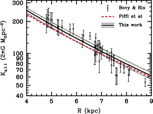
The vertical force 1.1 kpc from the Galactic plane as a function of radius for our main models, with 1σ uncertainties (solid and dashed lines, respectively), for the best-fitting model of Piffl et al. (2014a) (dashed red line), and from the fits to individual mono-abundance populations of Bovy & Rix (2013) (points with error bars).
Fig. 12 also shows the values of Kz, 1.1(R) found by Bovy & Rix (2013) (scaled such that R0 = 8.2). While the scatter of points around our model appears consistent with the error bars, there is a clear trend for the points at R ≲ 7 kpc to lie above the line from our model and the points at R ≳ 7 kpc to lie below it. The values of Kz, 1.1(R) found by Bovy & Rix (2013) are from individual ‘mono-abundance populations’, treated independently, and as coming from a single quasi-isothermal distribution function with an exponential density profile. The values given by Bovy & Rix (2013) and plotted in Fig. 12 are from the radius where a given mono-abundance population gives the tightest constraint, but each population provides constraints over a wide range of radii. The constraints provided by these different populations are not mutually consistent. The points in Fig. 12 therefore give the statistical uncertainty for each population at the radius where it is smallest, while there is clearly a systematic error (otherwise the different constraints would be consistent), which may be due to the assumption that each mono-abundance population is well described by a quasi-isothermal distribution function. This may explain the difference between the points in Fig. 12 and the two sets of lines.
McGaugh (2016) used a mass discrepancy–acceleration relation to relate the terminal velocity curve to a disc surface density profile. The vertical force at 1.1 kpc found was broadly similar to that found by Bovy & Rix (2013)– see McGaugh's fig. 14 - - but with more ‘bumps and wiggles’ and noticeably even further below the Bovy & Rix (2013) values for 5.5 kpc ≲ R ≲ 6.5 kpc than our model.
7.3 Streams and the shape of the dark-matter halo
Because of the large number of streams found in the Milky Way halo in recent years, it has become increasingly popular to attempt to constrain the potential of the Milky Way by fitting the properties of these observed streams to models. It is important to note that these streams are formed when satellites of the Milky Way are tidally disrupted, putting the stars that were in the satellite on to differing orbits. The difference between the motion on these orbits is the primary influence on the observed structure of the stream (Eyre & Binney 2011).
Gibbons, Belokurov & Evans (2014) find a very low mass for the Milky Way out to 100 kpc of (4.1 ± 0.4) × 1011 M⊙ by modelling the Sagittarius stream. This is significantly lower than other estimates (see Bland-Hawthorn & Gerhard 2016, table 8). It is worth noting that the comparison between model and data was entirely based on the positions of the apogalactic points of the leading and trailing tails of the stream, and the precession angle between them. It is not clear whether the model can explain the other properties of the Sagittarius dwarf. The study of the Sagittarius stream by Johnston, Law & Majewski (2005) had best-fitting models with masses in the range (3.8 − 5.6) × 1011 within 50 kpc, which is in keeping with our prior. We therefore treat this result with caution, and merely note that it differs substantially from the value we find for the mass inside 100 kpc of (8.2 ± 1.1) ± 1011 M⊙. If it is supported by further results we will have to re-evaluate our assumptions and find new models.
Küpper et al. (2015) used the position of apparent overdensities in the tidal tails of Palomar 5 to determine the mass within its apogalactic radius. However, Ibata, Lewis & Martin (2016) used deeper photometry of these tidal tails to demonstrate that these overdensities are very likely to be observational artefacts associated with inhomogeneities in the SDSS photometry used to produce the maps of Palomar 5 used by Küpper et al. (2015) (see also Thomas et al. 2016).
The flattening of the Milky Way's dark-matter halo remains deeply uncertain. Famously, models of the Sagittarius stream have been used to argue that the dark-matter halo is oblate (e.g. Johnston et al. 2005), prolate Helmi (2004) or triaxial (Law & Majewski 2010, though this is effectively oblate with the short axis in the plane of the Galaxy). Analysis of the smooth stellar halo as seen by the SDSS survey has yielded claims of constraints on the shape of the equipotential surfaces of the halo ranging from oblate with axis ratio |$q_\Phi = 0.7\pm 0.1$| (corresponding to axis ratios in the density distribution of 0.4 ± 0.1; Loebman et al. 2014) to prolate with axis ratio |$1.5\lesssim q_\Phi \lesssim 2$| (Bowden, Evans & Williams 2016). Analysis of the GD-1 stream, meanwhile, has yielded flattening estimates |$q_\Phi \sim 0.9$| (Bowden, Belokurov & Evans 2015). In the Solar neighbourhood, Read (2014) noted that the comparison of constraints from the rotation curve (which provides an estimate of the spherically averaged enclosed dark-matter content) and estimates of the local density provide a constraint on the halo shape which is consistent with spherical or slightly prolate. Piffl et al. (2014a) argued that combining their results with those of Bienaymé et al. (2014) provided tentative indications of an axis ratio (in the isodensity contours) of q ∼ 0.8. Piffl et al. (2014a) also noted that the axis ratio of the dark-matter halo has an important influence on the derived local density when interpreting dynamical models of the disc, with ρh, ⊙ ∝ q−0.89.
This is a deeply unsatisfying state of affairs, and we have followed numerous other authors in simply assuming that the dark-matter halo is spherically symmetric. This is an assumption that will need to be revisited to build a better model. Indeed, the assumption of a constant axis ratio at all radii will need examination. The argument of Read (2014), that comparing local and global constraints provides a route to solving this problem, indicates the role that approaches such as the one used in this study may have in the future. One must be careful, however, as this study has used a local constraint (from Kuijken & Gilmore 1991), so it is not suitable for making an unbiased comparison between the two approaches.
8 CONCLUSIONS
We have returned to the Bayesian methods laid out by Paper I, and used new data and an improved underlying model to find a new model of the mass distribution of the Milky Way. This new model includes components that represent the contribution of the cold gas discs near the Galactic plane, as well as thin and thick stellar discs, a bulge component and a dark-matter halo. We have used an MCMC approach to determine the properties of the models and their statistical uncertainties. We have also determined a best-fitting mass model, which provides a gravitational potential that can be used as a starting point in any dynamical modelling and for determining the orbits of stars in the Milky Way. We emphasize that this is an axisymmetric model, so cannot reflect the strongly non-axisymmetric bar structure in the inner few kpc of the Milky Way.
We have explored models that differ from the standard NFW halo density profile by allowing the density slope in the inner halo (γ in equation 5) to vary freely and fitting it to the data or by holding it at fixed values that differ from that of the NFW profile. If this is left as a free parameter, it is only weakly constrained γ = 0.79 ± 0.32. We have found that the local dark-matter density is surprisingly close to being independent of the assumed value of γ.
To explore possible systematic biases or overconfidence, we have explored models that include deviations from a purely exponential disc surface density. The effect on the virial mass is minimal, as is that to the derived values of R0 or v0, but an ∼10 per cent perturbation to the form of the surface density profile (which is at a level that is plausible) does produce a ≲ 10 per cent change in the derived local dark-matter density and the total stellar mass. We have explored other possible systematic uncertainties, and we would estimate that the systematic uncertainties (neglecting flattening of the dark-matter halo) are generally of the same order as the statistical uncertainties.
The value of R0 that we determine– 8.20 ± 0.09 kpc– is around 1σ lower than the one we take as our prior (Chatzopoulos et al. 2015), and if we take a weaker prior then the value of R0 is driven down still further, to ∼8.0 kpc. Since we know v0/R0 far better than we know v0 independently of R0, this remains an important uncertainty. The recent estimate of R0 ∼ 7.9 kpc from a new reduction of observations showing the orbits of stars around Sgr A* (Boehle et al. 2016) would appear to cast fresh uncertainty on this value when it seemed as if most estimates were tending towards ∼8.2–8.3 kpc (Bland-Hawthorn & Gerhard 2016).
We left the peculiar velocity of the Sun, |${\boldsymbol {v_{\odot}}}$|, and a typical peculiar velocity for the HMSFRs associated with the maser sources, as free parameters when fitting our models (though we place a prior on |${\boldsymbol {v_{\odot}}}$|). This allows us to investigate claims of a lag behind circular rotation associated with the HMSFRs, and whether there is any evidence that the peculiar velocity of the Sun found from stars in the Solar neighbourhood (by Schönrich et al. 2010) is inappropriate when looking at the larger scales of the Galaxy. We find no evidence of any significant lag associated with the maser sources. There is a strong degeneracy between the effect of a change to the assumed peculiar motion of the Sun and the assumed typical peculiar motion of the HMSFRs. We can therefore see that if U⊙ ∼ 14 km s−1 (as suggested by Schönrich 2012), the HMSFRs are typically moving radially inwards with a velocity of ∼6 km s−1, and if V⊙ ∼ 26 km s−1 (Bovy et al. 2012b) then the typical HMSFR leads circular rotation by ∼11 km s−1. We argue that such significant deviations from circular velocities are unlikely for these objects.
Code required to compute the properties of our models and to compute orbits within them has been made available at https://github.com/PaulMcMillan-Astro/GalPot, and in Appendix A we give a brief description of its use.
With the further release of data from Gaia, the number of stars for which we have accurate measurements of position and velocity is about to increase enormously. The data will enable us to improve our understanding of the Milky Way's structure dramatically and improve upon these models. As a summary of our understanding of the Milky Way's potential in the pre-Gaia era, the models provided by this study act as important starting point and should be used to estimate the orbits of the stars observed by Gaia, to help build our understanding of their place in the Galaxy.
Acknowledgments
The author is grateful to former colleagues in the Oxford Dynamics group, and to Justin Read, for helpful conversations in the early stages of this study, to Peter Kalberla for clarification regarding the gas content of the Milky Way, to Stacy McGaugh for a helpful tweet, to Ortwin Gerhard for helpful comments and to Louise Howes for careful reading of the finished paper. The research in this study is funded by the European Research Council, the Swedish National Space Board and the Royal Physiographic Society in Lund. The corner plots were created with the corner.py package (Foreman-Mackey 2016).
The software is available at https://github.com/PaulMcMillan-Astro/GalPot.
This is the same form as was used by DB98, but the expression given in the published journal version of that paper contains a typographical error (the term Rh/R is mistakenly given as Rh/Rd). This error does not appear in the arXiv version of the article: astro-ph/9612059.
There are varying definitions of the virial radius, and in this case the definition is the radius of a sphere with average density of approximately 94 times the critical density. We refer to this as |$c_{\rm v^\prime }$| rather than cv.
Fermani & Schönrich (2013) focused on different studies by the same lead authors, but the selection criteria used are similar or identical, so the points made are entirely relevant.
REFERENCES
APPENDIX A: galpot CODE AND ORBIT INTEGRATIONS
The galpot code is designed to provide the gravitational potential associated with axisymmetric density distributions like those used in this study. It was originally created by Walter Dehnen for the study of DB98, which contains a description of how it determines the potential and is available under a Gnu Public Licence. The version provided at https://github.com/PaulMcMillan-Astro/GalPot is there for convenience and includes files that provide the parameters for the potentials of our main model (Table 3), models with all of the variations shown in Table 6, the best-fitting model of Piffl et al. (2014a), the ‘best’ and ‘convenient’ models from Paper I and the four main models from DB98. We have included several example executables to demonstrate how this can be used, each of which provides helpful information about the required input if they are run without any arguments.
To use one of these potential in C++ code, one needs to enter the line
#include “GalPot.h”
in the declarations. Then, for example, to use our main model potential one could can use the code
ifstream from(“pot/PJM16_best.Tpot”);
Potential *Phi = new GalaxyPotential (from);
from.close();
The GalaxyPotential class can provide several useful properties of the potential (illustrated in the example executable testGalPot.cc), with the main ones being the potential and its derivatives at a point R, z, so for example the following code fragment
double R=8.2, z=1.1;
double P, dPdR, dPdz;
P = (*Phi)(R,z);
// or if derivatives needed too...
P = (*Phi)(R,z,&dPdR,&dPdz);
provides the potential at R, z (as P) and its derivatives with respect to R and z at that point (dPdR and dPdz, respectively). Note that it does not return the force per unit mass on an object at R, z (which is of course -dPdR and -dPdz in the two directions).
All inputs and outputs of GalPot are in the code units, which are radians, kpc, Myr and M⊙. Conversions are provided by the Units namespace (found in the file Units.h), and the format is that to put a value into code units you write ValueInCodeUnits = ValueInOriginalUnits * Units::NameOfUnit, so, for example
double v = 230. * Units::kms;
gives the variable v the value of 230 km s−1 in code units (note that this is ∼0.23 because 1 km s−1 ≈ 1 pc Myr−1). Equivalently, of course, one can write, for example
std::cout << v / Units::kms;
to convert back from code units and output the value in km s−1.
We also provide simple Runge–Kutta orbit integration routines to determine properties of orbits in a given potential. Example executable files demonstrate their use. For example, the executable findOrbitProperties.exe finds the properties of an orbit in our best-fitting model, given input initial R, z (in kpc) and vR, vz, vϕ (in km s−1). So, to find the properties of the Sun's orbit, taking R0 and v0 from Table 2, z0 from Binney et al. (1997) and the Solar peculiar velocity from Schönrich et al. (2010), one would run
./findOrbitProperties.exe 8.2 0.014 11.1 7.25 -245
and receive the output
Guiding Centre radius: 8.62121
Minimum, Maximum Cylindrical radius: 8.11988,9.18502
Maximum z: 0.104202
Minimum, Maximum Spherical radius: 8.12024,9.18521
Energy: -153122 km2/s2
Angular Momentum: -2009\,kpc km/s
Mean Cylindrical radius: 8.66851
The executable findManyOrbitProperties.exe does the same for a list of positions and velocities, in the same format, given in an input file, and outputs the results to a table.
The class OrbitIntegratorWithStats is used by these executables to determine statistics about the orbits. For example,
Vector <double,6> XV;
XV[0] = atof(argv[1]) * Units::kpc; // R
XV[1] = atof(argv[2]) * Units::kpc; // z
XV[2] = 0.* Units::degree; // phi unimportant
XV[3] = atof(argv[3]) * Units::kms; // v_R
XV[4] = atof(argv[4]) * Units::kms; // v_z
XV[5] = atof(argv[5]) * Units::kms; // v_phi
// Set up orbit integrator, with integration time
// 10000 Myr
OrbitIntegratorWithStats OI(XV,Phi,10000.);
// Run integration
int fail = OI.run();
if(fail) {
std::cout << “Orbit unbound”
} else {
// output statistics, e.g.
std::cout << “Maximum z:“<< OI.Maxz << “kpc\n”
}
To output the track for an orbit integration (at points roughly evenly spaced in time), one can use another function from OrbitIntegratorWithStats called runWithOutput, which is demonstrated in the executable findOrbit.exe. For example, to trace the orbit of the Sun, outputting 5000 points over the full integration (which covers 10 Gyr by default), one would run
./findOrbit.exe 8.2 0.014 0 11.1 7.25 -245 \
SunOrbit.tab 5000
The output table (in this case SunOrbit.tab) contains the full phase-space coordinates (R, z, ϕ, vR, vz, vϕ). The path in the R–z plane that this traces is plotted in Fig. A1.
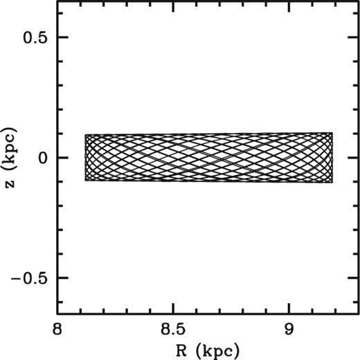
Trace of the Sun's orbit in the R–z plane as determined in the ‘best’ potential found in this study, using the executable findOrbit.exe. Only the first 1 500 points (representing 3 Gyr) are shown,
We also include code that can calculate coordinate transformations between commonly used coordinate systems, most notably galactic coordinates or equatorial coordinates. Conversions are done using the class OmniCoords, and demonstrations of its use are provided in the example executables, such as findManyOrbitPropertiesfromEquatorial.exe works in the same way as findManyOrbitProperties.exe but works in equatorial coordinates (by default, epoch J2000).
Note that by default OmniCoords assumes that the Sun is at R0 = 8.21 kpc, z0 = 0.014 kpc, that the circular speed at R0 is 233.1 km s−1, that the solar peculiar motion is that determined by Schönrich et al. (2010) and that equatorial coordinates are J2000. These can be changed before converting any coordinates as follows:
OmniCoords OC;
OC.change_sol_pos(8.3,0.025);
OC.change_vc(-244.5*Units::kms);
OC.change_vsol(10*Units::kms,5.25*Units:: kms,
7.17*Units::kms);
OC.change_epoch(2015.0);
Note also that the direction that the Sun rotates around the Galactic Centre is the negative ϕ-direction (to ensure that the Galactic north pole is the positive z-direction and the Sun is at ϕ = 0).
We also include code that can provide statistics on the orbits associated with observed stars, taking uncertainties into account. We provide an example executable called findManyOrbitPropertiesfromEquatorialwErrors.exe, which takes input in equatorial coordinates, with uncertainties (assumed to be Gaussian), and provides the parameters of the orbits, with uncertainties. It achieves this by Monte Carlo sampling within the uncertainties (with the number of samples chosen by the user) and integrating the orbits with the resulting starting positions and velocities to determine the orbital parameters. The statistics that are output are found as the median value from the Monte Carlo, with separate uncertainties in the positive and negative directions found by taking the 15.87 and 84.13 percentile values (the per cent equivalent of 1σ). It is worth noting that we have to take the median value, as the expectation value of many quantities (such as apocentric distance) is invariably infinite if the uncertainties are Gaussian. This is due to the fact that a finite change in any of the coordinates (which has a finite probability) can make the orbit unbound (and therefore having an infinite value of, e.g. apocentric distance). We also include code that derives the same properties for input coordinates that come from Gaia (i.e. parallax) or from the RAVE survey's multi-Gaussian fits to distance modulus pdfs.
The bulk of this code is also in the Torus Mapper (tm) package, and therefore described in section 2 of Binney & McMillan (2016). We have separated it out and added the utilities for orbit integration for ease of use (the galpot package is referred to as falpot in the tm package for historical reasons). However, it remains the case that better understanding and characterization of orbits come from the use of action-angle coordinates, which is beyond the scope of this simple package of code– see Sanders & Binney (2016) for a review of methods available for calculating actions.
