


Abstract
We study the correlation of galaxy structural properties with their location relative to the SFR–M* correlation, also known as the star formation ‘star-forming main sequence’ (SFMS), in the Cosmic Assembly Near-infrared Deep Extragalactic Legacy Survey and Galaxy and Mass Assembly Survey and in a semi-analytic model (SAM) of galaxy formation. We first study the distribution of median Sérsic index, effective radius, star formation rate (SFR) density and stellar mass density in the SFR–M* plane. We then define a redshift-dependent main sequence and examine the medians of these quantities as a function of distance from this main sequence, both above (higher SFRs) and below (lower SFRs). Finally, we examine the distributions of distance from the main sequence in bins of these quantities. We find strong correlations between all of these galaxy structural properties and the distance from the SFMS, such that as we move from galaxies above the SFMS to those below it, we see a nearly monotonic trend towards higher median Sérsic index, smaller radius, lower SFR density, and higher stellar density. In the SAM, bulge growth is driven by mergers and disc instabilities, and is accompanied by the growth of a supermassive black hole which can regulate or quench star formation via active galactic nucleus feedback. We find that our model qualitatively reproduces the trends described above, supporting a picture in which black holes and bulges co-evolve, and active galactic nucleus feedback plays a critical role in moving galaxies off of the SFMS.
1 INTRODUCTION
Out to z ∼ 3, galaxies can be split into star-forming and quiescent populations based on the bimodality observed in their colours and derived star formation rates (SFRs; Strateva et al. 2001; Kauffmann et al. 2003; Baldry et al. 2004; Bell et al. 2004; Brinchmann et al. 2004; Brammer et al. 2011; Ilbert et al. 2013). When focusing specifically on the galaxies classified as star forming, a strong correlation is observed between the SFR and stellar mass of galaxies at a fixed redshift (the SFR–M* correlation) (Daddi et al. 2007; Elbaz et al. 2007; Noeske et al. 2007; Rodighiero et al. 2011). This correlation is also sometimes referred to as the ‘star-forming main sequence’ (SFMS). This stands in contrast to the less rigidly defined quiescent population, for which there is no such strong correlation.
The SFR–M* correlation can be defined by a (redshift-dependent) normalization and slope, with a straight line in log–log space providing a reasonable fit, although there is evidence that the slope of the main sequence may flatten above a mass of ∼1010 M⊙ (Whitaker et al. 2012, 2014). It is still unclear whether this flattening is simply due to the fact that more of the stellar mass in high-mass galaxies is likely to be in a non-star-forming bulge component, as suggested by Abramson et al. (2014) or Tacchella et al. (2015), or whether there is something else going on. It has also been suggested that the presence of non-star-forming bulges in star-forming galaxies may increase the scatter in the SFR–M* relation around the main sequence (Whitaker et al. 2015). In any case, many studies have examined the SFR–M* correlation and found that it holds over at least four orders of magnitude in mass and exists out to z ∼ 6 [see Speagle et al. (2014) and references therein, as well as Salmon et al. (2015)]. The value of the slope in the SFR–M* plane is measured to be ∼1 (Rodighiero et al. 2011) and the relationship has an intrinsic 1σ scatter of only ∼0.2–0.4 dex (Whitaker et al. 2012; Kurczynski et al. 2016). In general, SFMS galaxies at high redshift have much higher SFRs than galaxies on the main sequence today (Sobral et al. 2014), and the evolution of the normalization of the SFMS appears to be independent of galaxy environment (Peng et al. 2010).
The small scatter of the SFR–M* correlation leads us to believe that galaxy evolution is dominated by relatively steady star formation histories rather than being highly stochastic and bursty. This places constraints on the duty cycle of processes such as galaxy mergers or disc instabilities, which may trigger starburst and quenching events that drive galaxies above or below the main sequence. Furthermore, observations show that since z ∼ 2 there has been a build-up of quiescent galaxies, while the mass density of galaxies on the SFMS has remained relatively constant, implying that galaxies are being moved off of the SFMS into the quiescent population, and remaining there permanently or at least over rather long time-scales (Bell et al. 2004, 2007; Borch et al. 2006; Faber et al. 2007). As the processes which move galaxies off of the main sequence are often associated with morphological change, it is interesting to examine the correlation between distance from the SFR–M* relation, or some other measure of quiescence, and galaxy structural properties.
Brennan et al. (2015, hereafter B15) defined a redshift-dependent SFMS by which to judge galaxies in order to divide them into star-forming and quiescent populations. We split the sSFR–Sérsic index plane into four quadrants in star formation activity and morphology: star-forming disc-dominated galaxies, star-forming spheroid-dominated galaxies, quiescent disc-dominated galaxies, and quiescent spheroid-dominated galaxies. After dividing galaxies up, we examined the evolution of the fraction of galaxies in each of these categories with redshift. In order to constrain which processes were responsible for moving galaxies between these different categories, we did the same analysis on a sample of model galaxies generated from the ‘Santa Cruz’ semi-analytic model (SAM) described in Somerville et al. (2008, hereafter S08) with updates as described in Somerville et al. (2012, hereafter S12) and Porter et al. (2014, hereafter P14). In addition to prescriptions for the main physical processes believed to be important for shaping galaxy properties (described below), the model includes bulge formation due to mergers and disc instabilities, and concurrent growth of supermassive black holes and active galactic nucleus (AGN) feedback, allowing us to predict how model galaxies evolve in the SFR–Sérsic index plane. The SAM is a useful tool for studying the evolution of large populations of galaxies, as it can generate large cosmologically representative samples with modest computational resources, allowing us to efficiently test the effects of various physical processes. In B15, we found that our prescriptions for quenching and morphological transformation were able to transform galaxies in a manner in qualitative agreement with the observations as long as bulge growth due to disc instabilities was included. Bulge growth due to mergers and disc instabilities and subsequent AGN feedback produced roughly the right fraction of galaxies in each of our four subpopulations. Models in which bulge growth occurred only due to mergers did not produce as many spheroid-dominated galaxies as seen in observations.
Our goal in this paper is to study the structural properties of model galaxies continuously across and off the main sequence rather than using the main sequence to sort our galaxies into bins based on their SFRs and morphologies as in B15 and Pandya et al. (2016). The latter explicitly examines galaxies with intermediate star formation and structural properties. We learned in B15 that our model could broadly produce the right fractions of different types of galaxies and the evolution of these fractions, and now we will examine more closely if it can both produce ‘typical’ main-sequence galaxies and match how the structural properties of galaxies change as they move farther from the main sequence. In this way, we hope to continue to build our understanding of the physical processes which drive the correlation amongst star formation, quenching, and galaxy structural properties.
Many observational studies have examined the structure of galaxies across the main sequence and come to several conclusions. (1) The main sequence is made up of kinematically and morphologically disc-dominated galaxies which have the largest radial sizes for their stellar masses (Williams et al. 2010; Wuyts et al. 2011, hereafter W11; Bluck et al. 2014; van der Wel et al. 2014b) (although it is true that the easy morphological distinction between disc-dominated and spheroid-dominated galaxies begins to break down at higher redshift, especially at high mass). (2) Galaxies lying above the main sequence are often morphologically disturbed and seem to be undergoing a starburst (W11; Elbaz et al. 2011; Salmi et al. 2012). Elbaz et al. (2011) suggest that some of these may also include heavily obscured AGNs. Of course, morphological disturbance above the main sequence is not universal (see Barro et al. 2016). (3) Compact star-forming galaxies [cSFGs; as defined in Barro et al. (2013)] on or just below the main sequence at z ∼ 2–3 suggest that bulge growth precedes quenching (Barro et al. 2014; Williams et al. 2014; Fang et al. 2015). Fang et al. (2015) even found that at z ∼ 2–3, cSFGs dominate the high-mass end of the main sequence. (4) Quiescence is almost always associated with a bulge component or high central stellar mass density or velocity dispersion (Franx et al. 2008; Bell et al. 2012; Wake, van Dokkum & Franx 2012; Fang et al. 2013; Bluck et al. 2014; Lang et al. 2014; Woo et al. 2015; Teimoorinia, Bluck & Ellison 2016). Estimates of galaxy black hole masses derived from central velocity dispersions also point to black hole mass being very correlated with quiescence (Bluck et al. 2016).
On the simulation side, Snyder et al. (2015) investigated the relationship amongst optical morphology, stellar mass and SFR for a sample of simulated galaxies from the Illustris simulation (Vogelsberger et al. 2014). They found that their model, which includes feedback from accreting supermassive black holes, was able to produce the population of quiescent bulge-dominated galaxies at z ∼ 0 needed to reproduce the distribution of observed morphologies. Tacchella et al. (2016) examined how galaxies in the VELA simulations (Ceverino et al. 2014) oscillate around the main sequence due to clumpy inflows and violent disc instabilities, leading to compaction and minor quenching episodes.
We compare our model predictions with galaxies observed with the Cosmic Assembly Near-infrared Deep Extragalactic Legacy Survey (CANDELS; Grogin et al. 2011; Koekemoer et al. 2011) and the Galaxy and Mass Assembly Survey (GAMA; Driver et al. 2011). In order to assure high levels of completeness and robust measurements of structural parameters, we only consider galaxies with stellar mass M* > 1010 M⊙, for both the models and observations. We consider several structural properties, including Sérsic index, size, stellar mass density and SFR density. In Section 2, we describe the SAM in more detail and give a summary of the observational data to which we will compare. In Section 3, we examine the distribution of structural properties across the SFR–M* plane, as in W11. We also examine how some quantities on which we currently do not have direct observational constraints, such as bulge-to-total luminosity ratio, black hole mass, and dark matter halo mass, vary across this plane. We next consider how these structural properties change as a function of linear distance from the main sequence, again as studied by W11. In Section 4, we investigate the distribution of distances from the main sequence in bins of galaxy structural properties following the analysis of Bluck et al. (2014). A secondary goal of the paper will be to compare our results to those of W11 and Bluck et al. (2014), the inspirations for several of our plots, where appropriate, and we discuss this in Section 5, along with a comparison between our model predictions and some other theoretical predictions in the literature. In Section 5 we also discuss what our model tells us about the Universe in the cases where our model and the observations agree, and what the Universe is telling us about our model in the cases where they do not. We summarize our results and conclude in Section 6.
2 SEMI-ANALYTIC MODEL AND OBSERVATIONAL DATA
2.1 The semi-analytic model
In this work, we use the same SAM as was used in B15, which was first presented in Somerville & Primack (1999) and Somerville, Primack & Faber (2001) and updated in S08, S12 and P14. This model has been shown to produce populations of galaxies that are in good agreement with observations; for comparisons with several statistical galaxy properties, see S08 and S12, as well as Lu et al. (2014) and Somerville, Popping & Trager (2015) for the evolution of the stellar mass function out to high redshift. A detailed look at the size–mass relation will appear in Somerville et al. (in preparation). As noted in B15, this model includes prescriptions for the hierarchical growth of structure, heating and cooling of gas, star formation, stellar population evolution, supernova feedback, chemical evolution of the interstellar medium (ISM) and intracluster medium (ICM) due to supernovae, and AGN feedback, as well as starbursts and morphological transformation due to mergers between galaxies and disc instabilities in isolated galaxies. We briefly summarize these processes below. For a more detailed description of the processes governing quenching and morphological transformation, see B15. For a more detailed description of the model in general, see S08 and P14. We assume a ΛCDM cosmology (Ωm = 0.307, ΩΛ = 0.693, h = 0.678) and a Chabrier (2003) initial mass function. We have adopted a baryon fraction of 0.1578. Our cosmology is consistent with the Planck 2013 results (Planck Collaboration et al. 2014) and was chosen to match that of the Bolshoi Planck simulation (Rodriguez-Puebla et al. 2016).
We use CANDELS mock lightcones (Somerville et al., in preparation) extracted from the Bolshoi Planck dark-matter N-body simulation (Klypin, Trujillo-Gomez & Primack 2011; Trujillo-Gomez et al. 2011; Rodriguez-Puebla et al. 2016). The ROCKSTAR algorithm of Behroozi et al. (2013a) is used to identify dark matter haloes. Merger trees for each halo in the light cone are constructed using the method of Somerville & Kolatt (1999), updated as described in S08. For our lowest redshift bin, we use a snapshot from the Bolshoi volume as opposed to the lightcone, which at that redshift represents a very small volume.
When dark matter haloes merge, the central galaxy of the largest progenitor becomes the new central galaxy, while all other galaxies become satellites. Satellite galaxies are able to spiral in and merge with the central galaxy, losing angular momentum to dynamical friction as they orbit. The merger time-scale is estimated using a variant of the Chandrasekhar formula from Boylan-Kolchin, Ma & Quataert (2008). Tidal stripping and destruction of satellites as described in S08 are also included.
Before the universe is reionized, each halo has a hot gas mass equal to the virial mass of the halo times the universal baryon fraction. The collapse of gas into low-mass haloes is suppressed after reionization due to the photoionizing background. We assume the universe is fully reionized by z = 11 and use the results of Gnedin (2000) and Kravtsov, Gnedin & Klypin (2004) to model the fraction of baryons that can collapse into haloes of a given mass following reionization.
When dark matter haloes collapse or are involved in a merger that at least doubles the mass of the progenitors (a 1:1 merger), the hot gas is shock heated to the virial temperature of the new halo. The rate at which this gas can cool is determined by a simple spherical cooling flow model (see S08 for details) which approximates the transition from ‘cold flows’, where cold gas streams into the halo along dense filaments without being heated, to ‘hot flows’, where gas is shock heated on its way in, forming a diffuse hot gas halo before cooling (Birnboim & Dekel 2003; Kereš et al. 2005; Dekel & Birnboim 2006). In this way, virial shock heating is included in our SAM, although many studies show that this effect alone is not enough to produce the observed population of massive quiescent galaxies (Somerville & Davé 2015, and references therein).
2.1.1 Star formation, bulge-formation and AGN feedback
There are two modes of star formation in the model: a ‘normal’ mode that occurs in isolated discs and a ‘starburst’ mode that occurs as a result of a merger or internal disc instability, as discussed below. The normal mode follows the Schmidt–Kennicutt relation (Kennicutt 1998) and assumes that gas must be above some fixed critical surface density (the adopted value here is |$6\, \,\mathrm{M}_{{\odot }}\,\rm {pc}^{-2}$|) in order to form stars.
Newly cooled gas collapses to form a rotationally supported disc, the scale radius of which is estimated based on the initial angular momentum of the gas and the profile of the halo. We assume that angular momentum is conserved and that the self-gravity of the collapsing baryons causes the inner part of the halo to contract (Blumenthal et al. 1986; Flores et al. 1993; Mo, Mao & White 1998).
Exploding supernovae and massive stars are capable of depositing energy into the ISM, which can drive outflows of cold gas from the galaxy. We assume that the mass outflow rate is proportional to the SFR and decreases with increasing galaxy circular velocity, in accordance with the theory of ‘energy-driven’ winds (Kauffmann, White & Guiderdoni 1993). Some ejected gas is removed from the halo completely, while some is deposited into the hot gas reservoir of the halo and is eligible to cool again. The gas that is driven from the halo entirely is combined with the gas that has been prevented from cooling by the photoionizing background and may later reaccrete back into the halo. The fraction of gas which is retained by the halo versus the amount that is ejected is a function of halo circular velocity as described in S08.
Heavy elements are produced by each generation of stars, and chemical enrichment is modelled simply using the instantaneous recycling approximation. For each parcel of new stars dm*, a mass of metals dMZ = ydm* is also created, which is immediately mixed with the cold gas in the disc. The yield y is assumed to be constant and is treated as a free parameter. Supernova-driven winds act to remove some of this enriched gas, depositing a portion of the created metals into the hot gas or outside of the halo.
Spheroids can be created by mergers or disc instabilities. Mergers between galaxies are assumed to remove angular momentum from the stars and gas in the disc and drive material towards the centre, building up a spheroidal component. In our model, this component is formed instantaneously. The size of the spheroid is determined by the stellar masses, sizes and gas fractions of the progenitors with the help of hydrodynamical binary merger simulations (see P14). This is a relatively recent addition to the model which gives much more accurate galaxy sizes. Velocity dispersions are also computed as described in P14. Mergers also trigger a starburst, the efficiency of which depends on the gas fraction of the central galaxy and the mass ratio of the two progenitors. The parametrization for the efficiency and time-scale of the burst is based on hydrodynamical simulations of mergers between disc galaxies (Hopkins et al. 2009). Stars formed as part of the burst are added to the spheroidal component, as are 80 per cent of the stars from the merging satellite galaxy. The other 20 per cent are assumed to be distributed in a diffuse stellar halo. We note here that the merger fraction in our model has been shown to be consistent with observational estimates in Lotz et al. (2011).
Disc material can also be converted into a spheroidal component as a result of internal gravitational instabilities. A pure disc without a dark matter halo is very unstable to the formation of a bar or bulge, while massive dark matter haloes tend to stabilize a thin, cold galactic disc (Ostriker & Peebles 1973; Fall & Efstathiou 1980). When the ratio of dark matter mass to disc mass falls below a critical value, the disc can no longer support itself and material collapses into the inner regions of the galaxy (Efstathiou, Lake & Negroponte 1982). Here we adopt an avenue for bulge growth due to disc instability, based on a Toomre-like stability criterion, which can be found in P14 or B15. As with mergers, the creation of the bulge component is instantaneous. This is another relatively recent addition to the model, but an important one as was shown in B15. In that work, we toggled the disc instability on and off. As we found that the model including disc instabilities was more successful in reproducing the morphological mix of galaxies seen in CANDELS and the local Universe, we focus almost exclusively on that one here.
Galaxies are initially seeded with a massive black hole of 104 M⊙ (Hirschmann et al. 2012). This black hole is allowed to grow by accretion and merging with other black holes, particularly as a result of galaxy mergers and disc instabilities. The prescription for this growth is described in B15 and in more detail in Hirschmann et al. (2012). In the case of mergers, the accretion rate is based on hydrodynamical binary merger simulations (Hopkins et al. 2006, 2007). For disc instabilities, the black hole is allowed to feed on some fraction of the mass which is moved to the spheroidal component, here 10−3, as in Hirschmann et al. (2012). In these cases, the black hole enacts feedback in the form of radiatively efficient, or ‘quasar’ mode, AGN activity. It is also able to feed and effect feedback in the ‘radio’ or ‘maintenance’ mode, during which it feeds via Bondi–Hoyle accretion from the galaxy's hot halo (Bondi 1952).
2.2 Computing Sérsic index and composite size for model galaxies
In this work, we compare the structural properties of model galaxies to those of observed galaxies. Our main basis of comparison is the Sérsic index; although, as mentioned above, disc-dominated and spheroid-dominated galaxies at high redshift become less morphologically distinct, the Sérsic index should still provide us with information about whether we are dealing with an extended or more compact galaxy. Our model directly computes the bulge luminosity, total luminosity, bulge radius and disc radius for each galaxy, allowing us to compute the bulge-to-total H-band flux ratio and bulge radius-to-disc radius ratio. The bulge radius and disc radius are recorded by the model as the 3D half-mass radius of stars in the bulge and the 3D scale radius of stars and cold gas in the disc, respectively. For our high-redshift galaxies (z > 0.5), we convert these quantities to projected rest-frame V-band half-light radii (the projection done according to Prugniel & Simien 1997) in order to use the stellar mass and redshift-dependent wavelength correction provided by van der Wel et al. (2014a) to get observed frame H-band sizes to go with our H-band bulge-to-total ratio (and to match the observed H-band Sérsic indices and sizes from CANDELS). The sizes of our low-redshift model galaxies are left in the rest-frame V band, which should be comparable to the r band from which the structural properties of GAMA galaxies are derived. We then utilize a lookup table generated by creating synthetic galaxies that are composites of n = 1 (disc) and n = 4 (spheroid) components, and then fitting a single-component Sérsic profile to the synthetic image (see Lang et al. 2014 for details). The table is parametrized in terms of bulge-to-total ratio and the ratio of the effective radii of the bulge and disc components. The output is an effective Sérsic index and effective radius for the composite system. The table contains discrete values so we use a 2D interpolation. The Sérsic index and effective radius that we derive here are lightweighted, in contrast to the stellar mass weighted quantities used in B15, and should provide a more accurate comparison to the Sérsic indices and sizes derived from light for our observed sample. However, we note that we do not attempt to include the effects of dust attenuation in our lightweighted quantities. We find that adopting these lightweighted quantities does not qualitatively change our results relative to B15, but does result in a significant improvement in the agreement between our models and the observations.
2.3 Observational data
2.3.1 High redshift: CANDELS
Our high-redshift data set (spanning 0.5 < z < 2.5) consists of observations taken as part of the CANDELS (Grogin et al. 2011; Koekemoer et al. 2011). The CANDELS data span five different fields and in this work we use data from all five: COSMOS (Nayyeri et al., in preparation), GOODS-N (Barro et al., in preparation), GOODS-S (Guo et al. 2013), EGS (Stefanon et al., in preparation), and UDS (Galametz et al. 2013) (see these references for details about data processing and catalogue creation for each of the CANDELS fields.) With this multi-wavelength data we are able to study the star formation properties and structure of galaxies out to z ∼ 2.5 at high resolution.
We make use of data catalogues generated by several previous studies. Here we give a very brief overview of the derivation of physical parameters which applies generally to all of the CANDELS fields (for more details, see B15 and Pandya et al. 2016). For a given field, the template-fitting method TFIT (Laidler et al. 2007; Lee et al. 2012) was used to merge data sets of different wavelengths with different resolutions in order to construct the observed-frame multi-wavelength photometric catalogue. The Bayesian framework of Dahlen et al. (2013) was used to derive photometric redshifts. Spectroscopic redshifts are used where available and reliable. 3D-HST grism redshifts are used for GOODS-S galaxies where available (Morris et al. 2015). The eazy code (Brammer, van Dokkum & Coppi 2008 and Kocevski et al., in preparation) was used to fit templates to the observed-frame SEDs in order to derive rest-frame photometry. Several independent codes, such as fast (Kriek et al. 2009), were used to derive stellar masses under fixed assumptions, but allowing for some variation of assumed star formation histories. We assume the following: Bruzual & Charlot (2003) stellar population synthesis models, Chabrier (2003) initial mass function, exponentially declining star formation histories, solar metallicity and a Calzetti (2001) dust attenuation law. A ladder of SFR indicators prescribed in Barro et al. (2011) and W11 is used to derive SFRs for galaxies in each field as described in B15 (see section 2.2.1 of that work). Finally, structural parameters were derived using galfit (Peng et al. 2002), fitting to the HST/WFC3 F160W H-band images using a one-component Sérsic model as described in van der Wel et al. (2012).
We make the following selection cuts on our data: stellar mass >1010 M⊙ (to ensure completeness) and galfit quality flag = 0 (to ensure good fits and robustness of our galaxy morphologies). We cut at a stellar mass of 1010 M⊙ for continuity with our low-redshift GAMA sample, which starts to become incomplete below this mass range. Because of this, we employ a relatively conservative mass cut throughout this work.
2.3.2 Low-redshift sample: GAMA
At low redshift CANDELS probes a very small volume, so we supplement with observations from Data Release 2 (DR2) of the Galaxy and Mass Assembly survey (GAMA; Liske et al. 2015). Our low-redshift range spans 0.005 < z < 0.12, sometimes referred to as z = 0.06 in the text. GAMA has an area of 144 deg2 and goes two magnitudes deeper (r < 19.8 mag) than SDSS while maintaining high spectroscopic completeness (≳98 per cent). GAMA also has a rich supplementary multi-wavelength data set (Liske et al. 2015). The backbone of GAMA is deep optical spectroscopy with the Anglo-Australian Telescope (AAT), while its multi-wavelength catalogues are bolstered by collaborations with several other independent surveys (for a review, see Driver et al. 2011).
Again, we make use of derived properties generated by previous work. Bulk flow-corrected redshifts are adopted from Baldry et al. (2012), and rest-frame photometry and stellar masses were derived from SED fitting as described in Taylor et al. (2011). GAMA's high spectroscopic completeness allows the derivation of Hα-based SFRs from extinction-corrected Hα line luminosities. Structural properties of GAMA galaxies are provided via multi-band measurements using galfit (Peng et al. 2002). We adopt the structural fits in the r band so as to analyse the structural properties of GAMA galaxies in the same band in which they were selected (as with the H band for CANDELS galaxies).
We also employ the following selection cuts as we did with our CANDELS data: stellar mass >1010 M⊙ (again to ensure our sample is complete) and galfit quality flag = 0.
2.4 Defining the main sequence
We define the main sequence much as we did in B15, although this time we use log(SFR) instead of log(sSFR). As described in B15, we decide to define our own stellar mass and redshift-dependent main-sequence line that is determined by the mean SFRs of galaxies. The SFRs of observed galaxies are systematically slightly higher than those of model galaxies, so this line is calculated separately for observed and model galaxies. While this already means that our model galaxies are not behaving exactly as observed galaxies, we do not think it impedes our goal of examining galaxy properties relative to the main sequence; as we judge quantities in this paper as a function of distance from the main-sequence line, we do not expect the disparity in absolute SFRs to affect our results.
We calculate the average SFR of galaxies with stellar masses between 109 and 109.5 M⊙ in time bins in order to measure the baseline main-sequence SFR across cosmic time, as we do not believe galaxies of this mass will be contaminated by objectively quiescent galaxies. In the models, we only use central galaxies. We then calculate the main-sequence slope by measuring the change in the mean log(SFR) between stellar masses of 109 and 109.5 M⊙. In each redshift bin, we use the mean low-mass SFR and derived slope to define a mass-dependent main-sequence line. While the SFR–M* correlation is known to have some dispersion, in order to judge distance from the main sequence, we define it with a single line, as has been done in W11 and Bluck et al. (2014). We also note that while the observed main-sequence slope is known to flatten towards higher stellar mass (Whitaker et al. 2012; Lee et al. 2015; Schreiber et al. 2015), here we extrapolate the slope derived for lower stellar mass galaxies to higher mass. We do this following the interpretation that the decrease in slope at higher stellar mass is due to the higher probability the galaxies of larger mass are already starting to quench and move off of the main sequence. Here, we try to define a more ‘pristine’ version of the main sequence, which we expect on theoretical grounds based on the fact that models without quenching have an unbroken linear SFR–M* correlation [see Renzini & Peng (2015) for another alternative to defining an unbiased main sequence]. Throughout this work, distance from the main sequence is given in units of log(SFR).
2.5 Evolution of star-forming galaxies versus quiescent galaxies in the SAM
Fig. 1 shows the evolution of the average SFR of galaxies from our model with cosmic time. The blue lines correspond to galaxies that are considered star forming at z = 0 according to the prescription described in B15 (meaning their SFRs are greater than 25 per cent of main-sequence SFR described above), while the red lines correspond to quiescent galaxies at z = 0 (with SFR <25 per cent of the main-sequence SFR). Galaxies have been split into two mass bins at z = 0, with final stellar masses ∼1010 M⊙ (109.9–1010.1 M⊙) or 1011.5 M⊙ (1011.4–1011.6 M⊙), representing the two ends of the mass range we are considering. We see evidence for the SFR–M* correlation in the higher SFR for star-forming galaxies of higher stellar mass (right panel) versus that of the lower stellar mass galaxies in the left panel. We also see an overall decrease in the SFRs of massive galaxies with cosmic time after an early peak at ∼2–3 Gyr. The SFRs of the less massive galaxies are only now beginning to decrease. We see the same type of behaviour for the quiescent galaxies, with the higher mass quiescent galaxies exhibiting an earlier and stronger peak.
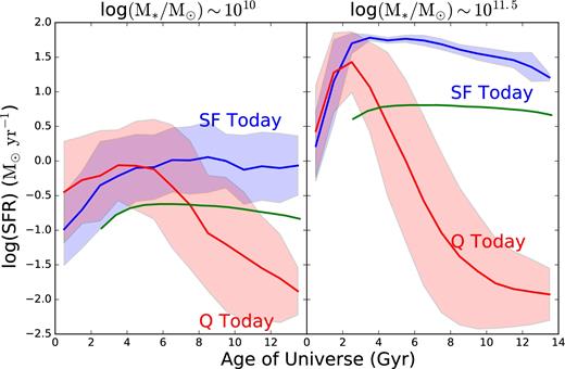
Evolution of the mean SFR for model galaxies that are star forming or quiescent in the present day, split into two mass bins. The blue lines indicate star-forming galaxies at z = 0, while red indicates quiescent galaxies at z = 0. The shaded regions correspond to the 1σ scatter in SFR for each of the curves. The green lines indicate the time-dependent star formation cut-off line, below which galaxies are considered quiescent at a given age of the universe. Left panel: Galaxies with stellar masses ∼1010 M⊙ at z = 0. Right panel: Galaxies with stellar masses ∼1011.5 M⊙ at z = 0. We see the main sequence of star formation manifested in the higher SFRs of more massive galaxies. We also see evidence of downsizing in the SFRs of more massive galaxies, which peak earlier than those of less massive galaxies. This is true for both galaxies that are star forming today, and for quiescent galaxies which peak at early times before falling below our quiescence threshold.
The scatter in SFR for quiescent galaxies is in general larger than that for star-forming galaxies because the mechanism that leads to the most intense quenching, AGN feedback, is associated with significant mass growth due to the major and minor mergers that trigger it. This is not as apparent in the low-mass panel, but only because we have artificially put a floor at log(SFR) = −2.0. Otherwise, the mean quiescent SFR became much less well-behaved.
This difference in average star formation histories between star-forming and quiescent galaxies is indicative of the SFMS at work in our model. As discussed in B15, and mentioned above, the SFR–M* correlation in our model does not behave exactly as that observed in the Universe; while the slope and normalization of our model main sequence are not quite the same as the observed SFR–M* correlation, we do reproduce a relationship between SFR and stellar mass. Galaxies tend to stay near this sequence until something happens to move them off of it, and the diversity of processes responsible, as well as the varying severity of these processes, leads to the larger spread in average star formation histories of galaxies that are quiescent today. Later, we will examine different galaxy properties as a function of distance from this SFMS, but first we will look at how different galaxy properties are distributed in the SFR–M* plane.
3 DISTRIBUTION OF PROPERTIES IN THE STAR FORMATION RATE–STELLAR MASS PLANE
Here we examine how the median Sérsic index, effective radius, SFR density, and stellar mass density vary across the SFR–M* plane for both our model and the observations. We note again here that for the rest of this work we impose a floor on log(SFR) so that all log (SFR) < −2.0 are set equal to −2.0. This is mainly to deal with quiescent model galaxy SFRs which would be far below the plots otherwise.
3.1 Number density in the SFR–M* plane
In Fig. 2, we show the distribution of galaxies in the SFR versus stellar mass plane. The number density is shown in grey-scale with contours overlaid in red. We also show the main-sequence fits we derive for both the model and observations in the three redshift bins of interest, as well as comparisons with the main sequence derived in Whitaker et al. (2012, 2014). We see immediately where the GAMA survey begins to become incomplete below a stellar mass of 1010 M⊙, which is why we have cut at this mass. We find that the distribution of galaxies is somewhat different in the model than in the observations. At all redshifts, most quiescent galaxies in our models have SFRs that are below our floor value log (SFR) = −2.0, while in the observations there is a cloud of galaxies with SFRs that are low enough to qualify them as ‘quiescent’ but well above our floor value.
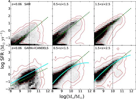
The distribution of model (top) and observed (bottom) galaxies with stellar mass >108 M⊙ in the plane of SFR versus stellar mass in the redshift bins z ∼ 0.06 (left panels), 0.5 < z < 1.5 (middle panels), and 1.5 < z < 2.5 (right panels). The grey-scale indicates population density with contours overlaid in red. The green lines show our fits to the main sequence of star formation, which are based on the mass range 109 to 109.5 M⊙ (solid green) and extrapolated to higher and lower masses (dashed green). The cyan lines indicate the main-sequence fits found in Whitaker et al. (2012) (lowest redshift bin) and Whitaker et al. (2014) (two higher redshift bins). The fits in Whitaker et al. (2014) are for smaller redshift bins, so we averaged the coefficients of the fits that fell within our larger bins. We see, as mentioned above, where the main-sequence slope becomes more shallow at higher stellar mass. The dashed black lines show the stellar mass cut we use for the rest of this work. We note that the normalization and slope of the SFMS are slightly different in the models and in the observations, which is why we fit them separately. In addition, we note that the distributions of SFR for quiescent galaxies are quite different in the models and observations. We discuss this further in the main text.
This may be due to limitations in our modelling of gas inflows and AGN feedback (for example, we may not resolve short time-scale rejuvenation events), or it could be due to the difficulty of obtaining accurate observational estimates of SFR for quiescent galaxies (while there is no explicit floor on detected SFRs in CANDELS or GAMA, the errors at low absolute SFR can become quite large and a natural floor is set based on the upper limits of detection in the photometric band used to derive the SFR). Despite this difference, we see that the main-sequence fits seem reasonable given the underlying distributions and continue with our analysis, although we will remark throughout when it seems this underlying difference is responsible for deviations between our model and the observations. We will also discuss possible reasons for this difference in our Discussion section.
3.2 Sérsic index in the SFR–M* plane
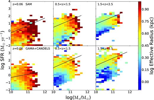
In Fig. 3, we explore the distribution of the Sérsic index in the SFR–M* plane by examining a colour map of the median Sérsic index in bins of SFR and M* (as in the analysis of W11, to which we compare directly in Section 6.1.1). The top panel shows this distribution for galaxies from our model and the bottom panel shows galaxies from the GAMA and CANDELS surveys. We have estimated the 1σ uncertainty on the median Sérsic index in each observational bin due to uncertainties in the estimates of galaxy properties in our observational sample. As in B15, we use quoted uncertainties in the Sérsic index and effective radius, an assumed uncertainty of 0.25 log(SFR) for SFRs, and the redshift-dependent stellar mass uncertainty of Behroozi, Wechsler & Conroy (2013b). The uncertainty, dn, in almost all bins and across all redshifts is only ∼0.0–0.3, except for at high redshift for low SFR galaxies, where dn∼ 1.0. In our lowest redshift bin, there is also a small patch of low SFR massive (>1011 M⊙) bins with dn ∼ 2.0. With this in mind we see that the model and observational distributions are qualitatively quite similar, although there are a few key differences.
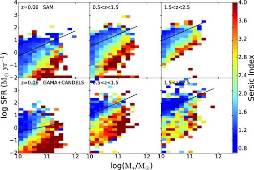
Distribution of median lightweighted Sérsic index in the SFR–M* plane for (top) model galaxies and (bottom) observed galaxies in three redshift bins. The black lines indicate the SFMS fits. We find good qualitative agreement between the model predictions and the observations, although our model does not exactly reproduce the distribution of structural properties across the main sequence. In addition, massive high Sérsic index (n ∼ 4) galaxies are more strongly quenched in our models than in the observations.
Both the model and observations exhibit a pocket of high Sérsic index at low SFR and high mass, although this trend is more pronounced in the observations, especially in the two lower redshift bins. As noted before, more galaxies in the models ‘pile up’ at SFRs below our floor value than in the observations, and these galaxies primarily have high Sérsic index (n ∼ 4) characteristic of very spheroid-dominated galaxies. In the observations, high-Sérsic index (spheroid-dominated) galaxies are predominantly quiescent, but have higher SFRs than their model counterparts. In addition, the quiescent population is dominated by galaxies with higher Sérsic index in the observations than in the models (see also Fig. 9).
Both the observations and model exhibit a smattering of high Sérsic index galaxies along the top edge of the SFR–M* distribution, above the main sequence, although this is more apparent in the observations. In our models, we know that galaxies like these are star bursting as the result of a merger and appear as bulge-dominated. However, we see that many of the highly star-forming galaxies above the main sequence in our model appear instead to be disc-dominated. The difference is especially apparent in the middle redshift bin, where some of the most massive, star-forming galaxies appear to have very strong discs. This is also true on the main sequence, where there appears to be a sharper transition to bulge-dominated systems along the observed main sequence (at ∼1011 M⊙ in our lowest redshift bin) than we see in the model.
In Fig. 4, we show the distribution of Sérsic index across the SFR–M* plane for our model without the prescription for bulge growth via disc instability. We see here how important the disc instability is in producing bulge-dominated galaxies. Without it we have very few truly bulge-dominated systems, even at low redshift far below the main sequence. Our main sequence is also completely dominated by disc galaxies, even at the high-mass end, unlike in the observed sample. The distribution of galaxies in the SFR–M* plane as compared with Fig. 3 is relatively unchanged; the disc instability is much more important for building bulge components than it is for quenching galaxies (See also B15, where it is shown that the quiescent fraction of galaxies changes very little between the two models, while the spheroid-dominated fraction changes by a significant amount.).
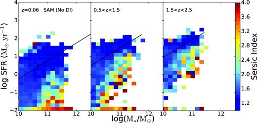
Distribution of Sérsic index in the SFR–M* plane for model galaxies in three redshift bins, in a version of the model that does not include bulge growth due to disc instabilities. The black lines indicate the SFMS fits. Here we see how important the disc instability mechanism is to building bulges in our model galaxies. Without it, we have very few bins with a median Sérsic index ≳3.5.
3.3 Sizes and surface densities in the SFR–M* plane
Fig. 5 is the same as Fig. 3, but for log effective radius. We calculate the uncertainty in each bin again as we did for Sérsic index and find that in general it is only ∼0.05 dex. In our lowest redshift bin at very high stellar mass, the uncertainty can grow to be ∼0.5 dex, but this affects very few bins. Again, the models qualitatively match the observations, although our model galaxies at low redshift tend to be too large. The main features are that there is a clear sequence from compact to extended galaxies from left to right, simply reflecting the size–mass relation. There is no clear correlation between size and location in the SFR–M* plane for galaxies that are near the SFMS (see also Shanahan et al., in preparation). However, galaxies that are below the SFMS (quiescent galaxies) are more compact at almost every mass than SF galaxies (although at our highest masses, even galaxies below the main sequence tend to be quite extended; we will return to this in Section 4, as well as the issue of our large low-redshift galaxies). These observational trends are well known (see e.g. van der Wel et al. 2014b, and references therein) and our models qualitatively reproduce them. We discuss the quantitative comparison between our model predictions and observational results in more detail in Section 4.
Distribution of log median effective radius in the SFR–M* plane for (top) model galaxies and (bottom) observed galaxies in three redshift bins. The black lines indicate the SFMS fits. The agreement between model and observations is qualitatively quite good, although at low redshift, our model produces galaxies that are too large.
Fig. 6 is the same as Figs 3 and 5, but now looking at the distribution of median SFR surface density, ΣSFR, defined as SFR/2πr2, where r is the effective radius. The uncertainty on these median values is generally less than ∼0.5 dex. Here again we see very good qualitative agreement between our models and the observations, the biggest difference being the high-density bins sitting above the main sequence that are much more pronounced in the observations than in the model. Whereas at z = 0.06, the model has no bins with a median log(ΣSFR)≳1.0 even at high redshift, the observations show several high SFR bins with log(ΣSFR) as large as 1.5 all the way down to low redshift. This may reflect limitations in our modelling of starburst systems.
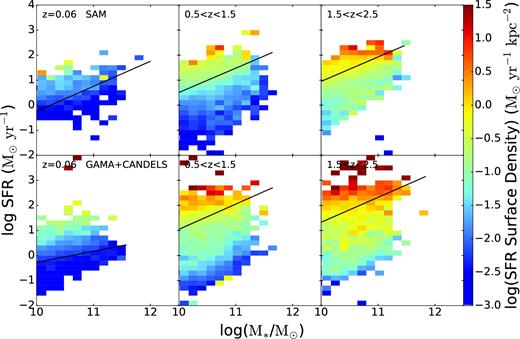
Distribution of median SFR density in the SFR–M* plane for (top) model galaxies and (bottom) observed galaxies in three redshift bins. The main difference between the model and the observations in all redshift bins is the absence of the highest SFR density systems in the model as compared with the observations. This is due to the on average slightly larger radii of the model galaxies above the main sequence, where the most concentrated observed galaxies are.
Fig. 7 shows the distribution of the median stellar mass surface density, |$\Sigma _{{M_{{\ast }}}}$|, defined as M*/2πr2 in the SFR–M* plane. The uncertainties on the median values here are less than ∼1.0 dex. We find that our agreement is very good in the lowest redshift bin. At higher redshifts, we see more compact systems in the observations, mainly below the main sequence at high stellar mass, than we produce in our model. This is most noticeable in our highest redshift bin. The most compact systems are those with n ∼ 4 in the quiescent cloud in Fig. 3.
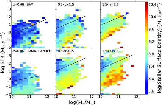
Distribution of median stellar mass density in the SFR–M* plane for (top) model galaxies and (bottom) observed galaxies in three redshift bins. The black lines indicate the SFMS fits. The qualitative agreement between the models and observations is very good, although the models do not reproduce as prominent a population of high surface density, quiescent galaxies in the highest redshift bin as seen in the observed distribution.
3.4 Model-only properties in the SFR–M* plane
In Fig. 8, we look at the distribution of some properties which are predicted for our models, but for which we do not currently have direct observational constraints. However, all of these quantities can in principle be observationally constrained. From top to bottom, these are bulge-to-total luminosity ratio (in observed F160W), bulge velocity dispersion, dark matter halo mass and black hole mass. The diagrams look extremely similar for all of these. As seen in previous studies, stellar mass is strongly correlated with all of these quantities, which also have significant correlations with one another. From this analysis, it is not possible to conclusively determine which property is the most fundamental causal factor in driving galaxy quiescence. We investigate this in more detail in a future work.
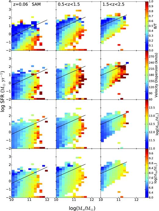
Distribution of (from top to bottom) bulge-to-total luminosity ratio in observed F160W, central velocity dispersion, halo mass, and black hole mass in the SFR–M* plane for model galaxies in three redshift bins. The black lines indicate the SFMS line fits. Here we see the behaviour of galaxy parameters which are native to our model, rather than the derived quantities we need to compare with observations. B/T and Sérsic index track each other very well. The other three quantities are strongly correlated with stellar mass.
4 DISTANCE FROM THE MAIN SEQUENCE
In order to be a bit more quantitative, we now examine the medians of the quantities investigated in the previous section as a continuous function of distance from the main sequence. We define ΔSFR as log(SFR)–log(SFRMS), where log(SFRMS) is the main-sequence SFR for a galaxy's stellar mass and redshift. A ΔSFR of ∼0 indicates galaxies on the main sequence, while a positive or negative ΔSFR indicates galaxies above (with a higher SFR than) or below (with a lower SFR than) the main sequence, respectively. The shaded region represents the distribution of the 25th–75th percentiles. We also include 1σ error bars derived the same way as the uncertainties on the median quantities in the last section. We set a floor for ΔSFR at a value of −3 dex, below which there are very few galaxies in either the models or the observations. We also employ somewhat larger bins towards lower ΔSFR to combat very low number statistics.
Fig. 9 shows median Sérsic index as a function of distance from the main sequence. In both the models and the observations, we see that the SFMS is dominated by galaxies with low Sérsic index (1.0–1.5), demonstrated by the minima of both the red and blue curves in all redshift bins near ΔSFR = 0 (recall that the intrinsic width of the SFMS is ∼0.2–0.4 dex). In the highest redshift bin, the SFMS population has slightly lower median Sérsic index (closer to a pure n = 1 exponential) in the observations, while in the models the median Sérsic index in this regime remains similar to the lower redshift bins. The trend towards increasing Sérsic index with decreasing ΔSFR seen in the observations is qualitatively reproduced in the models, as already noted, but the region below the SFMS (ΔSFR < 0) is dominated by galaxies with higher values of Sérsic index in the observations, at least in the two lower redshift bins. In the highest redshift bin, the models produce fewer quiescent galaxies than are seen, as already noted and discussed (also in B15). For the observations, there is a very slight upturn in median Sérsic index in the starburst regime of the SFMS (Δ SFR ≳0.6; e.g. Rodighiero et al. 2011) in the two lowest redshift bins. In the models, the highest ΔSFR bin is dominated by the few very highly star-forming, newly bulge-dominated systems, resulting in the large spike seen in all three redshift bins. These objects are rare in the model and subject to large statistical fluctuations in our relatively small samples, leading to the spikes as opposed to the gradual upturn of the observations. We also might expect the upturn in the observations to be larger (as seen in W11), but if the starburst is triggered by processes that cause morphological disturbance (such as mergers or disc instabilities), they are likely to have been excluded from our observational sample by our galfit quality cut.
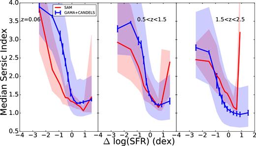
Median Sérsic index as a function of vertical distance from the fitted star-forming sequence for model galaxies (red) and observed galaxies (blue). The shaded region covers the 25th–75th percentiles of Sérsic index and the observations also have 1σ error bars reflecting the uncertainties in galaxy parameter estimation. Below the SFMS, both the model and the observations exhibit an increase in Sérsic index with increasing distance from the SFMS.
In Fig. 10, we see that our model in general produces galaxies whose sizes are in rough agreement with their observational counterparts in our two higher redshift bins, although in our lowest redshift bin, the model tends to produce galaxies which are too large regardless of distance from the main sequence. We also see that in the model, galaxies just above and below the main sequence tend to be slightly larger than galaxies directly on the main sequence; see the Discussion for more details. In our lowest redshift bin, and to a lesser extent in our middle redshift bin, the galaxies furthest below the main sequence tend to be especially large compared to observed galaxies; this will also be discussed later. In the observations, the largest galaxies live on the main sequence, with radial size decreasing monotonically below the main sequence with increasing distance from it.
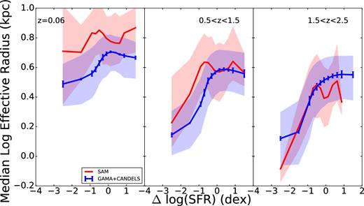
Median effective radius as a function of vertical distance from the fitted star-forming sequence for model galaxies (red) and observed galaxies (blue). The shaded region covers the 25th–75th percentiles of effective radius and the observations also have 1σ error bars reflecting the uncertainty in galaxy parameter estimation. At low redshift, our model galaxies tend to be too large.
Fig. 11 shows good agreement between the median values of ΣSFR at all distances from the main sequence in all three redshift bins, although model values fall slightly below observed values in our two higher redshift bins. In Fig. 12, we see that the model produces galaxies whose stellar mass surface densities are in decent agreement with those observed on the main sequence. Below the main sequence, where the model galaxies tend to be too large, as noted above, the stellar mass surface density falls below that found in the observations.
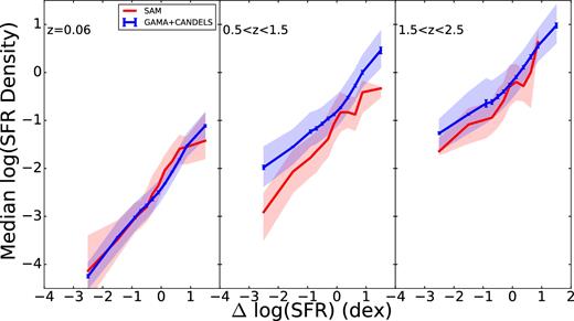
Median SFR density as a function of vertical distance from the fitted star-forming sequence for model galaxies (red) and observed galaxies (blue). The shaded region covers the 25th–75th percentiles of SFR density and the observations also have 1σ error bars reflecting the uncertainty in galaxy parameter estimation. The agreement between models and observations is in general quite good, although in our higher redshift bins, the models produce slightly less dense systems.
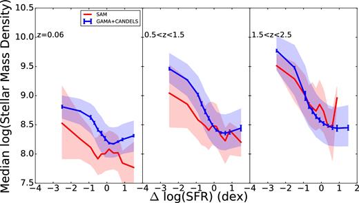
Median stellar mass density as a function of vertical distance from the fitted star-forming sequence for model galaxies (red) and observed galaxies (blue). The shaded region covers the 25th–75th percentiles of stellar mass density and the observations also have 1σ error bars reflecting uncertainty in galaxy parameter estimation. The agreement between the models and observations is generally quite good, with the largest deviation being ∼0.5 dex below the main sequence.
5 DISTRIBUTION OF DISTANCE AS A FUNCTION OF GALAXY PROPERTIES
Finally, we turn the tables and examine the distribution of ΔSFR in bins of various galaxy properties. Fig. 13 shows the results for stellar mass, bulge-to-total mass ratio, and halo mass at low redshift, for our models and for the analysis of SDSS galaxies by Bluck et al. (2014). The structural and stellar mass measurements for the SDSS galaxies were carried out by Simard et al. (2011) (bulge–disc decompositions by light) and Mendel et al. (2014) (bulge, disc and total stellar mass). For this plot and the next, we extend our mass range down to 108 M⊙, and use bulge-to-total stellar mass ratio as opposed to bulge-to-total luminosity ratio, to better compare with the results of Bluck et al. (2014). We see qualitatively similar trends, with the distributions for galaxies with larger values of these properties peaking below the main sequence. In the top left panel, we see a very extended model distribution for high-mass galaxies. Our model distributions have less well-defined peaks both on and off the main sequence than those seen for the observed galaxies in the top right panel. Bulge-to-Total stellar mass ratio (B/T) behaves the same way, although the model peaks are a bit more well-defined (but not as well as for the observations). The model distributions in bins of halo mass are well stratified, with higher halo mass galaxies peaking at successively lower ΔSFR. For the highest halo mass galaxies, this peak is right at our ΔSFR floor because these are most likely to be the most quiescent galaxies that live at the very bottom of our SFR–M* plane plots. The observed high halo mass distribution in the bottom right panel peaks at a higher ΔSFR because those galaxies live in the quiescent cloud like our quiescent GAMA and CANDELS galaxies do. As mentioned above, the lack of a distinct peak below the main sequence in these distributions (and those throughout this section) is due to the fact that we have arbitrarily low SFRs in our model, while it becomes very difficult to measure very low SFRs observationally. In fact, for the SDSS data with which we are comparing here, an explicit floor on specific SFRs [at log(sSFR) = −12.0] has been introduced (see Brinchmann et al. 2004 for details).
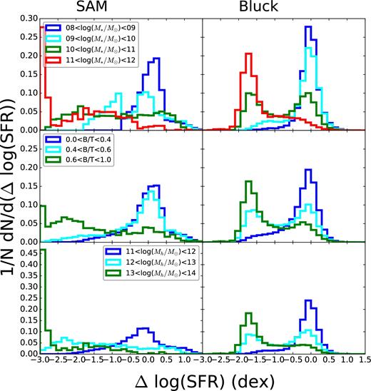
Distribution of Δlog SFR for different bins of galaxy properties (for galaxies with M* > 108 M⊙) in our lowest redshift bin. Left: model properties. Right: Galaxy properties used as part of the analysis of Sloan Digital Sky Survey galaxies that span the redshift range 0.02 < z < 0.2 in Bluck et al. (2014). Top panel: stellar mass. Middle panel: bulge-to-total stellar mass ratio (derived from bulge+disc decompositions for the observations). Bottom panel: halo mass (derived from abundance matching for the observations). All three of these quantities behave as expected. The model and the observations qualitatively agree, although the distributions for the larger values of each galaxy parameter tend to peak farther below the main sequence in our models than in the observations.
In Fig. 14, we see the same distributions for our higher redshift model galaxies. For all three galaxy properties, the distributions tend to collapse on to each other as we move to higher redshift, although stellar mass and halo mass remain somewhat stratified.
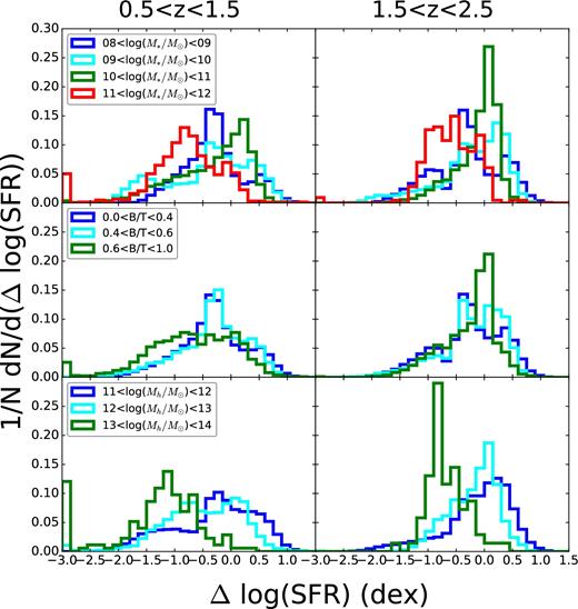
Distribution of Δlog SFR for different bins of model quantities (for galaxies with M* > 108 M⊙) in our two higher redshift bins (redshift increasing left to right). Top panel: stellar mass. Middle panel: bulge-to-total stellar mass ratio. Bottom panel: halo mass. We see that as we move towards higher redshift, the distributions in all bins of galaxy properties begin to pile up on the main sequence.
Now we return to the quantities we have been focusing on in the previous sections, comparing the distributions in bins of our model quantities with those from observed galaxies. We resume using our mass cut at 1010 M⊙ and revert back to using lightweighted B/T in order to derive the model Sérsic indices in the following plots. Fig. 15 shows these distributions in bins of Sérsic index, quartile of effective radius and SFR surface density for our lowest redshift bin. To assign a radius quartile, we divide galaxies into 1 dex mass bins (1010–1011 M⊙ and 1011–1012 M⊙) and see where they fall in the distribution of all sizes in their respective mass bins. We see that the qualitative agreement is good for all three quantities. Our model distributions tend to skew to lower ΔSFR as noted before. We also see that our model does not stratify in radius as well as the observations; we have some galaxies which are quite large for their stellar mass far below the main sequence and the distribution of large galaxies does not peak as strongly on the main sequence as it does for observations. We also see in the bottom panels that even our most dense star-forming systems are not as high above the main sequence as those seen in the observations. These conclusions are consistent with those we reached by looking at the plots of median quantities before.
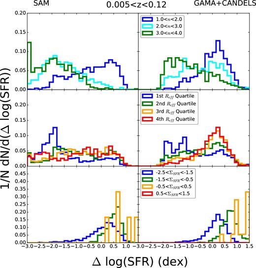
Distribution of Δlog SFR in our low-redshift slice for different bins of model (left column) and observed (right column) galaxy properties. Top panel: Sérsic index. Middle panel: quartile for effective radius for a given galaxy's 1 dex mass bin. Galaxies are divided into bins with 1010 < M*/ M⊙ < 1011 and 1011 < M*/ M⊙ < 1012. The first quartile is the smallest for each mass bin and so on. Bottom panel: SFR density. The agreement for all three quantities is very good, although our model distributions tend to have tails to lower ΔSFR than the observations.
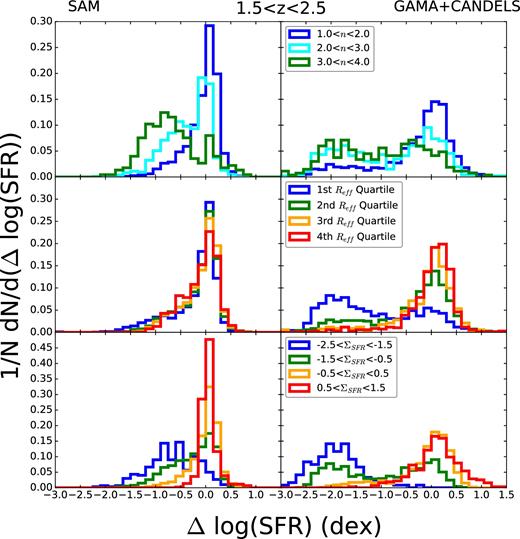
As we move towards higher redshift, the same trends persist. Fig. 16 is the same as Fig. 15 but for our middle redshift bin. The main difference we see is in the size distributions. While the observations show significantly different distributions in ΔSFR for the four radius quartiles, with the most compact galaxies being much more skewed towards large negative values of ΔSFR, the ΔSFR distributions in the models are much less well separated for the different radius quartiles. A similar result can be seen in Pandya et al. (2016), in which both model and observed galaxies have been split into star-forming, transition, and quiescent galaxies.

Distribution of Δlog SFR in our middle redshift slice for different bins of model (left column) and observed (right column) galaxy properties. Top panel: Sérsic index. Middle panel: quartile for effective radius falls into for a given galaxy's 1 dex mass bin. Galaxies are divided into bins with 1010 < M*/ M⊙ < 1011 and 1011 < M*/ M⊙ < 1012. The first quartile is the smallest for each mass bin and so on. Bottom panel: SFR density. Our agreement is again very good for Sérsic index and SFR density, but the models’ Δlog SFR distributions are not as well differentiated for different radius quartiles as they are in the observed distributions.
Finally, we look at high redshift in Fig. 17. Here, the lack of model quiescent galaxies at this redshift asserts itself. While our model reproduces the separation in the distributions in bins for Sérsic index, the high Sérsic index bins do not peak as far below the main sequence as in the observations. This is also true for the distributions in bins of SFR density. Our model does not reproduce the separation of distributions in bins of size quartile, with model galaxies of all sizes living near the main sequence. The high-Sérsic index, small-radius, and low-SFR density peaks seen below the main sequence in the observations are the beginnings of the quiescent cloud which our model has trouble reproducing.
Distribution of Δlog SFR in our highest redshift slice for different bins of model (left column) and observed (right column) galaxy properties. Top panel: Sérsic index. Middle panel: quartile for effective radius for a given galaxy's 1 dex mass bin. Galaxies are divided into bins with 1010 < M*/ M⊙ < 1011 and 1011 < M*/ M⊙ < 1012. The first quartile is the smallest for each mass bin and so on. Bottom panel: SFR density. The main disagreement in all panels is that our model distributions do not have a large enough quiescent population with SFR well below the main sequence.
6 DISCUSSION
Our study has demonstrated a significant correlation between galaxy structural properties and their star formation activity relative to a local SFMS. These correlations have been seen many times before both in the nearby Universe and out to high redshift. However, our study is novel in several respects. (1) We take particular care to carry out the analysis of the GAMA survey of nearby galaxies and the CANDELS survey out to z ∼ 2.5 in a consistent manner. (2) We carry out our analysis on the WFC3 images from the full five fields of CANDELS for the first time. (3) We make detailed comparisons between these observations and a statistically representative sample of model galaxies from a cosmological model of galaxy formation and evolution. The latter point is key, as an observed correlation can never prove causation, while if we see similar correlations in models, we can at least suggest a plausible story for a causal picture. For a brief discussion on progenitor bias and how this might affect the causal picture, see Section 6.2.3.
In this section, we compare and contrast the results of our analysis with previous results in the literature, and discuss what we have learned about galaxy evolution in the Universe and in our models.
6.1 Comparison with literature results
6.1.1 Comparison with the observational analysis of Wuyts et al.
The study by W11 was a primary inspiration for this work, and our observational analysis is deliberately very similar. For the most part, our conclusions are also very similar. Here we summarize the most important differences between the two studies. The structural measurements used in W11 were based on the ACS I814 image in the 1.48 deg2 COSMOS field, the H160 image in the CANDELS UDS and GOODS-S fields, and the z850 image in the GOODS-N field. Similarly, the catalogues used in W11 were selected in different filter bands and for different depths, as summarized in table 1 of W11. In contrast, our structural measurements are all derived from the CANDELS H160 image and are based on H160-selected catalogues with uniform depth for all five CANDELS fields. W11 computed their own photometric redshifts and stellar masses based on compilations of ground and space-based data from the literature for each of their fields, while we use the CANDELS team photo-zs and stellar masses for all five fields.
In spite of these differences, the main results of our analysis are very much in agreement with those of W11 overall. Here we highlight a few differences and some possible reasons for them. Comparing the bottom row of our Figs 3 and 9 with figs 1 and 2 of W11, one of the main differences we notice is the more pronounced population of galaxies with high Sérsic index, n ∼ 3.5–4, above the SFMS in W11. There are two possible reasons for this.1 First, our galfit quality cut eliminates galaxies with highly uncertain Sérsic index fits. W11 did not make such a cut and so includes star bursting systems that may have disturbed morphologies and may not be well fitted by a single Sérsic profile. If we remove this cut, we also see more star bursting systems above the main sequence in our observational sample. Secondly, the COSMOS ACS observations used by W11 cover a much larger area than the CANDELS WFC3 footprint and includes more rare objects such as starburst galaxies and massive, quiescent, very bulge-dominated galaxies. Comparing our Figs 5 and 10 with W11 figs 3 and 8, W11 saw a slightly stronger decrease in size for galaxies above the main sequence than we do. Similarly, W11 see more galaxies with very high SFR density (log ΣSFR > 1; figs 4 and 8) which again are missing from our sample. These compact, starbursting objects are likely the same ones that we have just discussed.
6.1.2 Comparison with other observational studies
We find that we are in qualitative agreement with several observational studies that have been done on the relationship between star formation and galaxy structural properties. As shown above, we find a similar segregation in the SFR–M* plane due to bulge mass or B/T stellar mass ratio as found in Bluck et al. (2014), the inspiration for the plots in our Section 5. We are also in qualitative agreement on this front with Lang et al. (2014) who found this type of segregation in CANDELS/3D-HST data (see also a comparison with our model in that work). Omand, Balogh & Poggianti (2014) found a simple dependence of quiescent fraction on B/T by flipping the type of analysis done here; they looked at the quiescent fraction in bins across the stellar mass–bulge fraction plane and found complementary behaviour to what we have found. Wake et al. (2012), Teimoorinia et al. (2016) and Bluck et al. (2016) all find strong dependence of star formation on central velocity dispersion at low redshift, as we see in the left panel of the second row of our Fig. 8. Woo et al. (2013) see segregation in the SFR–M* plane due to halo mass, which we also see quite strongly in the bottom panel of Fig. 13. Our results are also in qualitative agreement with those of Woo et al. (2015) who examined the distribution of sSFR for galaxies in bins of Σ1kpc (analogous to our Sérsic index) with fixed halo mass and vice versa.
6.1.3 Comparison with other theoretical studies
Many studies based on SAMs have shown that bulge-dominated galaxies in massive haloes tend to be red and quiescent (S08; Bower et al. 2006; Croton et al. 2006; Kimm et al. 2009; Lang et al. 2014), in general qualitative agreement with our results. As shown by e.g. Kimm et al. (2009) and Lang et al. (2014), different SAMs produce different relative degrees of correlation of the fraction of quenched galaxies with halo mass and bulge mass, reflecting differences in the physical recipes responsible for quenching star formation in the models. However, we are not aware of any other SAM-based comparison that has examined the continuous distribution of galaxy structural properties in the SFR–M* plane as we have done here.
Such an analysis has been done for the Illustris numerical hydrodynamical simulations at z = 0, by Snyder et al. (2015). The top left panel of their fig. 5 is strikingly similar to our redshift zero panel from Fig. 3, although it should be kept in mind that their colour coding is based on a different metric representing how bulge-dominated the galaxy is (Gini-M20). Similarly, in their fig. 10, Snyder et al. (2015) show that quiescent galaxies are more compact at a given mass than star-forming galaxies, although they note that the sizes of galaxies in Illustris are systematically too large. Snyder et al. (2015) show that quenching in the Illustris simulations is clearly associated with the growth of a massive SMBH as well as a massive halo, very similar to what we find in our SAMs. Snyder et al. (2015) have not presented a detailed comparison with observations. In another Illustris-based analysis, Sparre et al. (2015) showed that their simulations were lacking in extreme starburst galaxies (outliers above the SFMS), similar to what we find in our SAMs. The predicted population of extreme starbursts is likely quite sensitive to numerical resolution as well as the treatment of the ISM and feedback.
In another type of study, Zolotov et al. (2015) and Tacchella et al. (2016) analysed the SFRs and sizes of a set of high-resolution ‘zoom-in’ simulations. These 26 moderately massive haloes are not representative of a cosmological sample, and have not been run past z = 1, but they attain considerably higher resolution and contain arguably more physical ‘sub-grid’ recipes for processes such as star formation and stellar feedback than large cosmological volumes like Illustris. Zolotov et al. (2015) and Tacchella et al. (2016) emphasize that in their simulations, mergers and violent disc instabilities can lead to rapid gas inflow, building a compact, dense nucleus. They find that this ‘compactification’ phase is in general soon followed by a rapid decrease in SFR due to the changing decreasing inflow rate relative to the stellar-driven outflows. These authors also emphasize the role of building up a massive halo that can support a virial shock in driving the onset of quenching. However, these simulations do not include AGN feedback. This is likely the reason that, as noted by these authors, galaxies in these simulations do not ‘fully quench’. It can be seen in fig. 8 of Tacchella et al. (2016) that the simulations contain very few galaxies that are more than 1 dex below the SFMS, while the CANDELS observations show a significant population of such ‘strongly quenched’ galaxies even at 1.5 < z < 2.5. Fig. 8 of Tacchella et al. (2016) shows that within ±0.5 dex of the SFMS, galaxies in their simulations have a weak dependence of structural properties (stellar mass density, radius, Sérsic index) as a function of main-sequence residual. This is in qualitative agreement with our SAM predictions, and with the CANDELS observations. It also suggests that in order to create the strong outliers from the SFMS seen in observations, additional physical processes (such as AGN feedback) accompanied by fairly dramatic structural transformation are likely needed.
6.2 Interpretation of results
Overall, our model's agreement with observations is qualitatively very good, although there are some recurring issues which manifest many times in the above analysis. We now discuss both sides of this coin: what does our model tell us about the Universe when the two agree with each other, and what does the Universe tell us about our model when they do not?
6.2.1 What our model tells us about the Universe
The broad agreement between our model and the observations is extremely encouraging and suggests a plausible physical scenario that can explain the observed correlations. In this picture, relatively smooth accretion of gas fuels star formation and builds up rotationally supported discs. The radial size of the disc that forms is roughly proportional to the angular momentum of the gas, which (on average) traces that of the dark matter halo. Relatively minor perturbations, such as minor mergers or disc instabilities, cause galaxies to oscillate around the SFMS as suggested in Tacchella et al. (2016), and seen also in our models. As long as galaxies remain in this relatively smooth undisturbed growth phase, their structural properties do not show a strong correlation with their distance from the SFMS.
Eventually, either through many small perturbations or a few larger ones (see e.g. fig. 14 of B15), a galaxy can build up a sufficiently massive black hole that AGN feedback prevents further significant cooling, perhaps also rapidly removing the star-forming ISM through powerful winds. In the models presented here, bulge growth and black hole growth are explicitly linked, and both are fed through a combination of major and minor mergers and disc instabilities. It is certainly not clear that the details of the implementation of these processes are correct in our simulations or any existing ones, but it is not unexpected that the build up of a dense central nucleus and rapid feeding of a SMBH should go together. In our models, this linked growth of a compact, dense structure in the centres of galaxies and the engine that drives feedback (the SMBH) is the causal driver of the strong correlations between structure and SFR for galaxies that are below the SFMS. It is plausible that this is also the case in the real Universe. We note also that although there is general consensus that what is sometimes called ‘halo quenching’ (the build up of a halo massive enough to sustain a virial shock) is not by itself sufficient to cause strong and long-duration quenching (Choi et al. 2015; Pontzen et al. 2016), it is certainly reasonable to suppose that any sort of AGN feedback will have an easier time stopping the accretion of hot, low-density, isotropically distributed gas than that of dense, cold, filamentary gas. Because the fraction of accretion via the ‘hot mode’ versus ‘cold mode’ increases strongly with increasing halo mass (Birnboim & Dekel 2003; Kereš et al. 2005; Dekel & Birnboim 2006), it may therefore be that some combination of halo mass and black hole mass is in fact the best indicator of whether the conditions for quenching are met (see Terrazas et al. 2016; also Snyder et al. 2015 and Woo et al. 2015). This will be an interesting issue to explore in simulations with more detailed treatment of AGN feedback.
Our model also suggests the existence of some rather radially large galaxies in the two lowest redshift bins most prominent in the left panel and below the main sequence in the middle panel of Fig. 10. These galaxies do not appear to be present in existing catalogues from GAMA or CANDELS, but an interesting question is whether these objects could be missed due to their very low surface brightness. The recent discovery of ‘ultra diffuse galaxies’ in the Coma and Virgo cluster (van Dokkum et al. 2015a,b; Koda et al. 2015; Mihos et al. 2015), as well as extremely large disc galaxies (Ogle et al. 2016), has called into question whether there might be more large, diffuse galaxies out there than previously thought. Using the effective soft surface brightness limit of GAMA [23.5 mag arcsec−2 in the r band; Baldry et al. 2012], we estimate that over 17 per cent of model galaxies in our lowest redshift bin with effective radii >10 kpc at least 1.5 dex below the main sequence would be undetected. About two-thirds of these are disc galaxies and the rest are spheroid dominated. A detailed comparison between our model predictions and the observed populations of ultra-diffuse galaxies is beyond the scope of this paper, but it is intriguing that our models predict there may be a population of large diffuse galaxies.
6.2.2 What the Universe tells us about our model
Unfortunately (or perhaps fortunately), the Universe does not take our suggestions on how to run itself, so here we discuss how our model is failing to reproduce the observations and what we may be able to learn from this. As discussed above, our most quenched galaxies, which are the result of intense AGN feedback after building a massive black hole, have SFRs which are lower than those in the quiescent cloud of observed galaxies. This probably indicates that our treatment of AGN feedback is too simple. Real galaxies likely undergo short duty-cycle bouts of quenching and rejuvenation, which our simple model does not resolve. Also, although the observed population of compact, high-central density starburst systems well above the SFMS fits into our theoretical merger-based picture, we have trouble actually producing enough of these systems when compared with the observations. This is a direct result of the treatment of star formation enhancement in merger-triggered bursts implemented in our SAMs, which was based on a now rather out-of-date set of hydrodynamic simulations of binary mergers. As noted above, other hydro-simulations, such as the Illustris simulation, have had similar trouble producing ‘extreme’ starbursts which we would expect to see far above the main sequence (Sparre et al. 2015). We expect future simulations with higher resolution and a more detailed treatment of the ISM will help us understand how this population is produced.
The slight peaks in radial size above and below the main sequence apparent in Fig. 10 appear to be due to highly star-forming galaxies which still have a significant disc component and disc-dominated galaxies which are slowly fading off of the main sequence, respectively. Examples of the discy highly star-forming galaxies can be found in the upper-rightmost occupied bins of the top middle panels of Figs 3 and 5. These galaxies, while likely starbursts, still have fairly low Sérsic indices and large sizes. A few galaxies like this are enough to cause the peak seen in Fig. 10, as we start to see fewer galaxies that far above the main sequence overall. The large galaxies just below the main sequence appear to be due to a slight difference in the 2D size distributions seen in Fig. 5. In the observational panels, we see that in the two higher redshift bins, for a given mass, as we move below the main sequence we only see sizes greater than or less than the sizes seen on the main sequence. In the model, however, at high stellar masses, especially, it is possible to encounter sizes larger than those found on the main sequence. Because this occurs at high mass and because the corresponding bins in Fig. 3 are fairly disc-dominated, it seems that these are fairly massive discs which have fallen below the main sequence but which are not yet quiescent. While we expect galaxies to be kept on the main sequence by these cycles of activity and relative dormancy, it appears that perhaps this cycle is affecting the sizes of our galaxies too strongly, as there is no sign of this size behaviour in the observations.
As noted above, we also find that our model produces quiescent galaxies that are somewhat larger than those observed, and this discrepancy increases with decreasing redshift (see Fig. 10). The systematic nature of this discrepancy in our lowest redshift bin suggests the need to refine overall how sizes are computed.
Finally, while it is possible that some of the large model galaxies in our lowest redshift bin might be missed observationally due to selection effects, this is likely not the full cause of the disagreement, especially for galaxies on the main sequence. Because disc galaxies are the largest galaxies for their mass range, it would be easy to assume that most of our very large galaxies are disc-dominated ones that escaped merging and were allowed to grow out of control. However, more than half of our model galaxies with sizes >20 kpc are in fact spheroid-dominated. This is doubtless due to the limitations of the relatively simple modelling of the sizes of discs and spheroids in our SAMs. A clue is that the sizes of our largest galaxies, regardless of morphology, are correlated with abnormally low halo concentrations. While the average halo concentration of our low-redshift sample is ∼8.5, when limiting to galaxies with effective radii >20.0 kpc we find an average halo concentration of ∼7.0. A more detailed investigation of the size–mass relation in our model and its evolution will be presented in Somerville et al. (in preparation).
6.2.3 Progenitor bias
Lilly & Carollo (2016) have suggested that the correlations between star formation and structural properties might be explained by progenitor bias. For galaxies at any epoch, quiescent galaxies represent systems that left the main sequence at an earlier epoch when the Universe was denser and galaxy sizes were characteristically smaller. Because of this, quiescent galaxies will be systematically smaller than galaxies that have continued to grow while on the main sequence, regardless of any relationship between quenching mechanism and galaxy structure. As noted above, we have been careful to make the distinction between correlation and causation in this work, but can look to our model for guidance. While progenitor bias exists in our model, as characteristic galaxy sizes grow with cosmic time, we find that we are unable to reproduce basic statistical galaxy properties like the stellar mass function, luminosity functions or stellar mass-to-halo mass relationship without including some form of feedback. Meanwhile, on the observational side, Bluck et al. (2016) have found that high central velocity dispersion is a good predictor for the fraction of green valley galaxies as well as for quiescent galaxies. Green valley galaxies are not as likely to have left the main sequence a long time ago like quiescent galaxies, suggesting that feedback is a better explanation for these systems than progenitor bias. In light of this, while we acknowledge that progenitor bias may be a factor in the structural correlations observed here, we believe our model still represents a plausible explanation for our observations.
7 SUMMARY AND CONCLUSIONS
In this work, we have investigated the correlation of galaxy structural properties with their location in the plane of SFR and stellar mass. We studied structural properties such as morphology as represented by the Sérsic index, radial size, and mean stellar surface density as a continuous function of a galaxy's distance from the mean SFMS at its observation time. We carried out a parallel analysis on the GAMA survey of nearby galaxies, the CANDELS survey, which can measure galaxy structural properties to z ∼ 3, and a SAM that tracks the evolution of galaxy properties within a cosmological framework. We focus on the population of galaxies with stellar mass >1010 M⊙, for which these surveys are highly complete and the measurement of structural properties is robust.
Our main findings are as follows.
Within ±0.5 dex of the SFMS, we find a weak dependence of galaxy structural properties on the distance from the MS. Below the main sequence, we see a rapidly steepening dependence such that galaxies with larger negative MS residuals had higher median Sérsic index, smaller size, and higher stellar surface density. These trends are seen in both nearby galaxies (GAMA) and out to z ∼ 2.5 (CANDELS), and are qualitatively very similar in the theoretical models.
Our observational results are very similar overall to the results of an earlier study by W11. One difference between our results and those of W11 is that we do not find a significant population of galaxies with high Sérsic index (n ∼ 3.5–4) in the extreme starburst region above the SFMS. Similarly, we do not see as large a population of galaxies with small radii above the SFMS. We suspect that these galaxies are removed from our sample due to our requirement of being well fitted by a single-component Sérsic profile.
The good qualitative agreement between our model results and the observations suggests a plausible causal explanation for the observed correlations, namely, that central spheroids and black holes grow together, and black holes play a major role in quenching star formation in galaxies.
Quantitatively, our models disagree with the observations in some important respects. Our models do not produce as large a quiescent population at high redshift (z > 1.5) as seen in the observations (as already noted by B15), and the SFR for the model quiescent galaxies is lower than those of observed quiescent galaxies. This suggests the need to refine our modelling of AGN feedback. Moreover, the Sérsic indices of galaxies below the SFMS are systematically lower (more disc-like) in the models, while on and below the SFMS, especially at low redshift, the sizes of our galaxies are too large. As a result, there is not as large a separation between the sizes for the star-forming and quiescent populations in the models as what is seen in the observations. This suggests that we also need to refine our determination of galaxy sizes in the model.
Acknowledgments
We thank the anonymous referee for a constructive and thought-provoking report. RB was supported in part by HST Theory grant HST-AR-13270-A. RSS thanks the Downsbrough family for their generous support and acknowledges support from the Simons Foundation through a Simons Investigator grant. Thanks to Asa Bluck for providing us with data; his analysis in his own paper was a partial inspiration of this work. We acknowledge the contributions of hundreds of individuals for the planning and support of the CANDELS observations, and to the development and installation of new instruments on HST, without which this work would not have been possible. Support for HST Programmes GO-12060 and GO-12099 was provided by NASA through grants from the Space Telescope Science Institute, which is operated by the Association of Universities for Research in Astronomy, Inc., under NASA contract NAS5-26555.
Note also that figs 2 and 8 of W11 plot a slightly different mass range than our corresponding figures.
