


Abstract
The survival of dust grains in galaxies depends on various processes. Dust can be produced in stars, it can grow in the interstellar medium and be destroyed by astration and interstellar shocks. In this paper, we assemble a few data samples of local and distant star-forming galaxies to analyse various dust-related quantities in low- and high-redshift galaxies, and to study how the relations linking the dust mass to the stellar mass and star formation rate evolve with redshift. We interpret the available data by means of chemical evolution models for discs and proto-spheroid (PSPH) starburst galaxies. In particular, we focus on the dust-to-stellar mass (DTS) ratio, as this quantity represents a true measure of how much dust per unit stellar mass survives the various destruction processes in galaxies and is observable. The theoretical models outline the strong dependence of this quantity on the underlying star formation history. Spiral galaxies are characterized by a nearly constant DTS as a function of the stellar mass and cosmic time, whereas PSPHs present an early steep increase of the DTS, which stops at a maximal value and decreases in the latest stages. In their late starburst phase, these models show a decrease of the DTS with their mass, which allows us to explain the observed anti-correlation between the DTS and the stellar mass. The observed redshift evolution of the DTS ratio shows an increase from z ∼ 0 to z ∼ 1, followed by a roughly constant behaviour at 1 ≲ z ≲ 2.5. Our models indicate a steep decrease of the global DTS at early times, which implies an expected decrease of the DTS at larger redshift.
1 INTRODUCTION
Interstellar dust represents the solid component of the interstellar medium (ISM), and it strongly affects several properties of galaxies. First of all, dust grains absorb and scatter the optical and ultraviolet (UV) radiation in the well-known dust-extinction process. Most of the light absorbed by dust at UV and optical wavelengths is then thermally re-emitted at much longer wavelengths, in the infrared (IR) band, where the dust-reprocessed radiation represents the major contributor.
Secondly, the depletion of refractory elements into dust grains has a considerable effect on the chemical composition of galaxies. In our Galaxy, the depletion levels are found to vary largely as a function of the density and temperature of the ISM (Savage & Sembach 1996; Jenkins 2009). This is true also in high-redshift damped Lyman alpha systems observed in quasar (QSO) and gamma-ray burst (GRB) absorption lines, which show strong evidence of dust depletion in heavy element abundances (e.g. Vladilo 2002; Calura, Matteucci & Vladilo 2003; Calura et al. 2009b).
Thirdly, dust grain can enhance radiative cooling of the ISM and thus directly affect the star formation history of galaxies, as well as the stellar initial mass function (IMF) by inhibiting the formation of massive stars (e.g. Omukai et al. 2005; Bekki 2013).
In galaxies, the survival of dust grains is regulated by a series of constructive and destructive processes, which take place on rather distinct time-scales. Dust grains are thought to form in the lowest temperature and highest density regions of stellar envelopes and of the ISM. Favourable conditions for dust formation are met in the rapidly expanding shells of the ejecta arising from supernova (SN) explosions, as well as in outer envelopes of asymptotic giant branch (AGB) stars, on time-scales ranging from a few Myr up to several Gyr (e.g. Dwek 1998; Tielens 1998; Edmunds 2001; Morgan & Edmunds 2003; Zhukovska 2014; Dell'Agli et al. 2015; Michalowski 2015). Dust grains are also destroyed in SN shocks (Barlow 1978; McKee 1989; Jones, Tielens & Hollenbach 1996; Schneider, Ferrara & Salvaterra 2004; Silvia, Smith & Shull 2010), on times as fast at ∼104 yr after the SN explosion (Gall, Hjorth & Andersen 2011a). Dust grains can also grow in the coldest phases of the ISM (Draine & Salpeter 1979; Draine 1990; Dwek, Galliano & Jones 2007; Pipino et al. 2011; Valiante et al. 2011; Asano et al. 2013; Schneider, Hunt & Valiante 2016), typically on typical time-scales a few tens of Myr (Michalowski 2015), i.e. of the order of the lifetime for local molecular clouds (Dwek 1998). Direct evidence for dust accretion comes from the observed increase of the depletion levels at large interstellar densities and low temperatures (e.g. Savage & Sembach 1996) and from the observed IR emission of cold molecular clouds (e.g. Steinacker et al. 2010), characterized by the absence of small-grain emission. These features can be accounted for by the coagulation of small grains on and into larger particles. Indirect evidence of dust accretion comes also from the estimation of the grain lifetimes, which would be very small if no process could allow them to recondense and grow (Draine & Salpeter 1979; McKee 1989).
In the last few years, extragalactic surveys in the IR and submillimetre (submm) bands allowed us to perform an accurate estimate of the dust mass budget in local and distant galaxies. Recent studies revealed that submm galaxies (SMGs) at redshift z > 1 generally show a larger dust content than local spirals and even ultraluminous infrared galaxies (ULIRGs; e.g. Santini et al. 2010; Fisher et al. 2014), hosting the most vigorous dust-enshrouded starbursts in the local Universe. Although a fraction of them has been resolved into multiple sources by ALMA observations (ALESS survey; Hodge et al. 2013), these surveys have revealed the difficulty to account for the large dust masses observed in high-redshift galaxies with standard assumptions regarding dust evolution (Morgan & Edmunds 2003, Dwek, Galliano & Jones 2007; Santini et al. 2010; Valiante et al. 2011; Rowlands et al. 2014), i.e. with choices for the most basic parameters regulating dust growth and destruction tuned by reproducing the content of dust in local galaxies, also including a standard (i.e. non-top-heavy) stellar IMF.
Even studies of QSO hosts at higher redshifts (z > 6) indicate the presence of large masses of dust in the early Universe, suggesting that the dust build-up has occurred on time-scales considerably lower than ∼1 Gyr (e.g. Maiolino et al. 2004; Wang et al. 2013; Calura et al. 2014), i.e. the age of the Universe at those redshifts. This implies that in these systems, the formation of dust was possible through processes likely faster than the lifetimes of intermediate-mass stars, characterized by initial mass 2 ≤ m/M⊙ < 8 and which at these epochs are still on the main sequence; hence, they did not have enough time to produce considerable amounts of dust grains (but see Valiante et al. 2009). Moreover, the large star formation rate (SFR) values of QSO hosts imply large destruction rates (Gall et al. 2011a; Mattsson 2011; Calura et al. 2014), as it has been widely reckoned that (SNe, the most rapid stellar dust factories (Dunne, Eales & Edmunds 2003), are more efficient dust destroyers than producers (Dwek 1998; Calura, Pipino & Matteucci 2008), and this outlines the counterbalancing, fundamental role of the interstellar growth to support such large dust masses (Mattsson 2011; Pipino et al. 2011; Valiante et al. 2011). On the other hand, the absence of dust in metal-free, low star formation objects at z > 6 and in the local universe (Fisher et al. 2014) implies a dichotomy between rapidly dust-rich and dust-free objects.
A still open question is the possibility that the build-up of dust may occur in lockstep with that of metals, as suggested by a recent discovery by Zafar & Watson (2013) of a constant, nearly solar dust-to-metal ratio in GRB and QSO absorbers, with very little dependence on column density, galaxy type or age, redshift, or metallicity. On the other hand, De Cia et al. (2013) find significant variations of the dust-to-metal ratio in both QSO and GRB absorbers, with the discrepancy between their results and those of Zafar & Watson (2013) likely due to an overestimate of the intrinsic dust content estimated from the line of sight AV, as done by the latter authors. These significant variations of the dust-to-metal ratio versus metallicity might be explained by means of a non-universal ratio between the stellar dust and metal yields related to a dependence on metallicity of the dust yields (Mattsson et al. 2014b).
In this paper, we assemble data sets from various IR and submm surveys across a wide redshift range (0 ≤ z ≤ 6), and we use published results to gain a deeper insight on the evolution of the dust mass budget throughout cosmic history. To this aim, we consider various dust-related galactic scaling relations and assess how they evolve with redshift. Our study is mostly focused on the amount of dust which is produced in galaxies per unit stellar mass, on how this quantity depends on the stellar mass and what are the main physical processes which drive its cosmic evolution. The observational data sets are compared to chemical evolution models for galaxies of different morphological types, which include a detailed treatment of dust production (Calura et al. 2008) and which allow us to put strong constraints on the relation between the quantities studied in this work and the underlying galactic star formation history.
2 THE OBSERVATIONAL DATA SET
In this paper, we focus on the stellar mass Mstar, the dust mass Mdust, the gas mass Mgas and the SFR. The data set includes sources from the literature spanning a wide redshift interval, for which some of the above physical quantities are available. For a subset of data, novel estimates of some of these quantities have been derived as explained below in Section 2.1.
The data have been homogenized according to the following prescriptions: (i) a Salpeter IMF for the stellar masses and the SFR; (ii) a fit with a modified blackbody (MBB) function for the dust masses (see Section 2.1). Finally, for the samples where both H i mass and molecular gas masses are available, the observed gas masses have been calculated as the sum of these two quantities. In the ULIRG and SMG samples, we assume that their total gas mass is coincident with their H2 mass.
2.1 Dust masses in the COSMOS and GOODS fields
We derived novel estimates of the dust masses for galaxies in the COSMOS, GOODS-S and GOODS-N fields from the PEP Herschel survey (Lutz et al. 2011), and we used the multi-wavelength data set and source classification assembled by Gruppioni et al. (2013) to derive the Herschel luminosity function.
We have considered only the sources for which the observed flux Sν was available for at least four photometric data points at λrest > 20 μm, and all the sources dominated by an AGN were removed [i.e. classified in Gruppioni et al. (2013) as type 1 and type 2 AGN]. A final sample of ∼2700 galaxies, in the redshift range 0.01 < z < 4.8, was obtained.
Bianchi (2013) discussed how the bulk of the dust mass in galaxies can be robustly determined from the emission in the range 100 ≤ λ ≤ 500 μm, by fitting a single-temperature MBB to the data. However, the use of an MBB fit for the spectra to estimate the dust masses might seem questionable, as dust grains may present vastly different sizes and a large diversity of heating sources.
Several authors have shown how stable fits to the data can be obtained also using a grain-temperature distribution (GTD; Kovács et al. 2010; Magnelli et al. 2012), as it has been shown that dust grains have to be characterized by a GTD and its assumption deeply affects the estimate of the dust mass (see e.g. Xie, Goldsmith & Zhou 1991; Xie et al. 1993; Li, Goldsmith & Xie 1999; Magnelli et al. 2012; Mattsson et al. 2015). In general, the assumption of a GTD leads to dust mass estimates larger than those obtained by means of an MBB fit by factors of 1.5–2 (e.g. Santini et al. 2014; Berta et al. 2016). For this reason, our estimates can be regarded as lower limits to the dust masses for the galaxies of our samples.
2.2 Other data sets used in this work
We have assembled two data sets at z ≲ 0.1: a sample of spiral galaxies and a sample of ULIRGs.
The spiral subsample includes 26 objects from the SINGS (Kennicutt et al. 2003), with full multi-wavelength photometry and also with submm data, useful for dust mass measurements. Estimates for the SFR, Mstar and Mgas were taken from Santini et al. (2010), and the H i and H2 mass estimates are from Kennicutt et al. (2003). The dust masses were re-calculated using an MBB fit.1 The dust masses measured with an MBB fit result to be a factor of 2–3 lower than those estimated by the grasil code or using the Draine & Li (2007) templates (see Santini et al. 2014).
A subset of 46 spirals were selected from the KINGFISH sample (Kennicutt et al. 2011). For these sources, Mstar and Mdust are from Skibba et al. (2011). The Mgas estimates have been calculated from the sum of the H i mass (Walter et al. 2008) and the H2 mass (Leroy et al. 2009).
The ULIRG sample consists of 24 systems, originally from Clements, Dunne & Eales (2010) and, as for the spiral SINGS sample, estimates for the SFR, Mstar and Mgas were taken from Santini et al. (2010) by considering a CO-to-H2 conversion factor [α = 4.3 M⊙ (K km s−1 pc2)−1] which applies to normal galaxies. No estimate for the H i mass is available for these systems. The dust masses have been re-computed by means of a fit with an MBB function, as explained earlier in Section 2.
At redshift z > 0, we use the sample of 24 SMGs presented by Santini et al. (2010). These sources are in the redshift range 0.5 ≤ z ≤ 4 and the estimates of Mstar and Mgas were taken from Santini et al. (2010), whereas the dust masses were re-computed as described above for the SINGS and ULIRG systems. We also consider one additional SMG source, SMMJ123600.15+621047.2 from Greve et al. (2005).
Finally, for our study of the dust-to-stellar mass (DTS) ratio as a function of redshift (Section 4), we also consider the sample of QSO host galaxies at z > 6 from Calura et al. (2014), to which the reader is referred for further details. This sample shows that at z ∼ 6 a significant amount of dust is already present in several IR-luminous QSO hosts. A transition in dust production could have occurred at slightly larger redshifts, perhaps somewhere between z ∼ 6 and z ∼ 7, given the compelling absence of dust found in a couple of systems at z > 7 (Ouchi et al. 2013; Inoue et al. 2016).
3 CHEMICAL EVOLUTION MODELS
The observational data sets described in Section 2 are compared with results from chemical evolution models for proto-spheroidal (PSPH) galaxies and spiral, disc galaxies. In this section, we present a brief description of the chemical evolution models used in this work. More detailed descriptions of the models can be found in Calura et al. (2009a, 2014), Schurer et al. (2009) and Pipino et al. (2011).
Elliptical galaxies are assumed to originate from the rapid collapse of a gas cloud with primordial chemical composition. During this ‘proto-elliptical’ phase, this rapid collapse triggers an intense and rapid star formation process, which lasts until the onset of a galactic wind, powered by the thermal energy injected by stellar winds and Type II and Type Ia SN explosions. At this time, the gas thermal energy equates the gas binding energy, and all the residual ISM is assumed to be lost. After this time, the galaxies evolve passively. The models considered in this work are designed to describe three PSPH galaxies of baryonic mass 3 × 10¹⁰, 1011 and 1012 M⊙.
We also consider a suite of chemical evolution models for spiral galaxies of three different baryonic masses, spanning from ∼2 × 10⁹ to 1011 M⊙ (Calura et al. 2009a). In such models, the baryonic mass of any spiral galaxy is dominated by a thin disc of stars and gas in analogy with the Milky Way. The disc consists of several independent rings, 2 kpc wide, without exchange of matter between them. The disc formation occurs ‘inside-out’, i.e. the time-scale for disc formation increases with the galactocentric distance (Matteucci & Francois 1989). In our models, we assume that the efficiency of star formation is higher in more massive objects which evolve faster than less massive ones, a behaviour known as ‘downsizing’ (e.g. Matteucci 1994; Cowie et al. 1996; Recchi, Calura & Kroupa 2009).
All the models for spiral discs and for PSPHs include stellar dust production, mostly from core-collapse SNe and intermediate-mass stars, restoring significant amounts of dust grains during the AGB phase. In this work, for all the refractory elements, we consider the set of metallicity-independent dust condensation efficiencies presented by Dwek (1998). For a discussion on the effects of metallicity on stellar dust production and its impact on galactic chemical evolution models, see Gioannini et al. (2017).
Dust destruction in SN shocks and interstellar dust accretion are also taken into account as described in Calura et al. (2008). The evolution of elliptical galaxies is followed during their star-forming phase only, i.e. in our scheme, before a galactic wind may occur. However, it is worth stressing that also galactic outflows may represent an efficient mechanism to remove substantial amounts of dust from the ISM (Calura et al. 2008; Feldmann 2015).
In Fig. 1, we show for our models, from the top-left panel and in clockwise sense, the star formation histories along with the time evolution of the gas mass, of the dust mass, of the dust-to-gas ratio, of the metallicity (here traced by 12 + log (O/H)) and of the DTS ratio. The results for the PSPH models were computed both assuming a standard, Salpeter (1955) IMF and a Larson (1998), top-heavy IMF (THIMF). For the spiral models, we adopt instead a Scalo (1986) IMF (see Section 3.1).
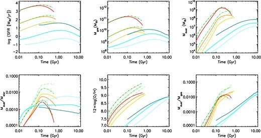
Clockwise, from top left: star formation history, evolution of the gas mass, of the dust mass, of the dust-to-gas ratio, of the interstellar metallicity and of the DTS ratio as a function of time for our chemical evolution models described in Section 3. In each panel, the yellow solid line, the orange solid line and the red solid line represent the PSPH models of baryonic mass 3 × 10¹⁰, 1011 and 1012 M⊙, respectively, computed with a standard, Salpeter (1955) IMF. The light green, green and dark green dot–dashed lines are for three PSPHs with the same baryonic masses as above but characterized by a top-heavy IMF (Larson 1998). The light cyan, cyan and dark cyan solid lines represent models for a dwarf spiral, an intermediate-mass spiral and an M101-like spiral, respectively (Calura et al. 2009a).
The downsizing character of the PSPH models is visible from the more extended SFHs in the less massive systems. The star formation (SF) is assumed to stop as soon as the conditions for the onset of the galactic wind are met, i.e. when the thermal energy of the ISM balances its binding energy.
In these models, the assumption of a THIMF generally produces larger dust masses (Gall et al. 2011a), larger metallicities (up by a factor of ∼0.5 dex) and larger DTS values than those achieved with a Salpeter (1955) IMF.
The three spiral models are characterized by lower SFRs and more prolonged star formation histories than PSPHs. As the spiral models are multi-zone, each of the quantities plotted in Fig. 1 represents the mass-weighted averages on the whole disc as described in Calura et al. (2009a) and considering only regions located at galactocentric distances 3 kpc < R < 8 kpc. As outlined by the recent Herschel Exploitation of Local Galaxy Andromeda, local disc galaxies are known to exhibit dust-to-gas and dust-to-metal gradients (Smith et al. 2012; Mattsson et al. 2014a). Even if such gradients are likely to be present also in high-redshift galaxies, in this work we assume that for each object of our sample, the observational quantities we compare our results with are luminosity-weighted values representative of the galaxy as a whole. Such an assumption may be justified by considering that, as the innermost parts are the densest and the most luminous, the average quantities computed within the regions located at radii R < 8 kpc could be regarded as representative of the entire discs (Calura et al. 2009a).
For the sake of consistency in the comparison with the observational gas masses described in Section 2, the gas mass Mgas refers to the total hydrogen mass present in the ISM in all models.
The entire set of models used in this work was successful in reproducing a few basic properties of galaxies and their evolution with cosmic time, such as the mass–metallicity (MZ) relation (Calura et al. 2009a) and the dust abundance pattern in galaxies of different morphological types (Calura et al. 2008; Schurer et al. 2009; Pipino et al. 2011). Recently, the PSPH models have been matched with spectrophotometric models which include the emission from dust grains to successfully account for the evolution of the K band and of the FIR luminosity functions across the redshift range 0 < z < 3 (Pozzi et al. 2015).
3.1 Initial mass function
In our standard PSPH galaxies, we adopt a Salpeter (1955) stellar IMF, i.e. a simple power law ϕ(m) ∝ m−1.35 constant in space and time, with stellar mass lower limit 0.1 M⊙ and upper limit 100 M⊙. This choice ensures that several observational constraints such as the average stellar abundances of present-day spheroids, the colour–magnitude diagram (Pipino & Matteucci 2004) and their global metal content (Calura & Matteucci 2004) are reproduced, as well as the metal content in clusters of galaxies and its evolution (see Renzini 2005; Calura, Matteucci & Tozzi 2007).
In spiral galaxies, the IMF is the one of Scalo (1986). This choice ensures that the abundance pattern observed in local spiral and disc galaxies is well accounted for (e.g. Calura & Matteucci 2004; Cescutti et al. 2007).
The use of this IMF is also motivated by various results showing that in general, the disc IMF must be significantly steeper than the cluster IMF, i.e. a universal Massey–Salpeter IMF with a Salpeter slope at the largest masses, i.e. at m ≥ 8 M⊙. This result stems from the fact that the integrated IMF of the disc population can be obtained from a folding of the universal IMF with the star-cluster mass function (e.g. Weidner & Kroupa 2005; Calura et al. 2010; Recchi & Kroupa 2015), which is well described by a single power law (Lada & Lada 2003).
Recently, Calura et al. (2014) showed that a Larson (1998) IMF with mc = 1.2 M⊙ in PSPHs produces an IMF richer in massive stars than the standard Salpeter IMF and allows one to account for the dust content of starbursts detected at z ∼ 6. In high-redshift starbursts mc = 1.2 M⊙ will be our reference value.
As discussed in Mattsson (2011), in principle, since observations suggest that low- and intermediate-mass stars produce significantly more dust per stellar mass than high-mass stars, if stars were the only sources of dust a THIMF would result in a lower total stellar dust yield. However, also processes other than stellar dust production are at play (such as dust growth) and overall the adoption of a THIMF implies larger dust amounts than those achievable with a normal IMF.
4 RESULTS
Various scaling relations for our galaxy samples at different redshifts are plotted in Figs 2 and 3, where the observational data sets described in Section 2 are compared with theoretical results from chemical evolution models of galaxies of different morphological types as described in Section 3. Combined together, the dust masses, the gas masses and the stellar masses allow one to have an insight on a few basic physical properties related to local and distant galaxies and on how some fundamental galaxy parameters evolve with redshift in the selected samples. The comparison with chemical evolution models is useful to interpret the data, since it can provide information on the possible morphology of the systems, and it also allows one to put constraints on their star formation history (Calura et al. 2009b).
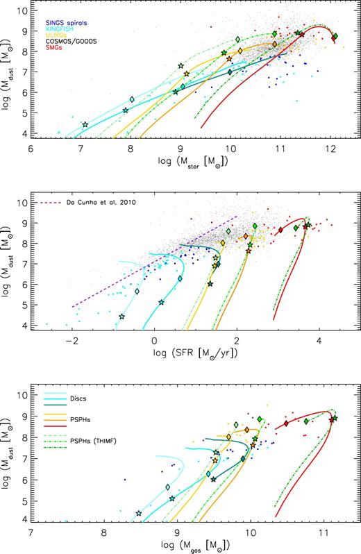
Upper panel: dust mass as a function of the stellar mass for the observational data discussed in Section 2. Symbols are colour-coded according to the different samples as follows. Blue circles are local spiral galaxies from the SINGS survey, light blue circles are local galaxies from the KINGFISH survey, yellow circles are local ULIRGs and red circles are SMGs from Santini et al. (2010), whereas the black dots are galaxies from the COSMOS/GOODS survey. The curves represent the models described in Fig. 1. The stars and diamonds plotted along each curve and with its same colour mark the evolutionary times of 0.1 and 0.5 Gyr, respectively. The central panel and the bottom panel show the observed and theoretical dust mass as a function of the SFR and the dust mass as a function of the gas mass, respectively. The purple dashed line in the central panel represents the Mdust–SFR relation found in local galaxies by da Cunha et al. (2010). All the other data and curves are as in the upper panel.
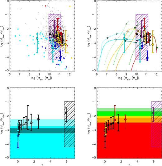
Top panels: DTS ratio as a function of the stellar mass. The large filled cyan, blue, yellow, red and black circles plotted with the error bars represent the median DTS values calculated in bins of stellar mass for the KINGFISH, SINGS, ULIRG, SMG and COSMOS/GOODS samples, respectively. The small purple squares are the DTS values measured in eight QSO hosts from the sample of systems at z ∼ 6 of Calura et al. (2014), i.e. in the systems for which it was possible to derive an estimate of the stellar mass. Note that in these systems, the stellar masses were computed from measures of the dynamical masses and neglecting the presence of dark matter and that if the latter was present, they should be regarded as upper limits. The large purple square with the error bar represents the median DTS value of the sample of Calura et al. (2014), as computed for these eight systems. The purple hatched area accounts for the non-detections of the z ∼ 6 sample (see Section 4.4 for details on its calculation). All the other curves and symbols are as in Fig. 2. All the median DTS values as a function of the stellar mass are reported in Table 1. Bottom panels: DTS ratio as a function of redshift. In the bottom-left panel, the filled cyan and blue circles are the median DTS values calculated for the local KINGFISH and SINGS samples, respectively, whereas the open symbols represent the median values calculated for higher redshift samples (see the description of the bottom-right panel). The light cyan, cyan and dark cyan regions in the bottom-left panels enclose the range of DTS values predicted for low-mass, intermediate-mass and larger mass spiral galaxies, respectively. In the bottom-right panel, the open circles with error bars are the median DTS as calculated for the local KINGFISH and KINGS samples, whereas all the other symbols with error bars are as in the top panels. The purple hatched area accounts for the non-detections of the sample of systems at z ∼ 6 of Calura et al. (2014); its width was calculated from the difference between the two extreme redshift values of the objects belonging to that sample. The yellow, orange and red regions in the bottom-right panel enclose the DTS values of the PSPH models of lower mass, intermediate-mass and larger mass, respectively, calculated assuming a Salpeter (1955) IMF. The light green and green regions in the bottom-right panel enclose the DTS values computed for the lowest mass and intermediate-mass PSPHs, respectively, computed assuming a THIMF. All the average DTS values as a function of redshift are reported in Table 2.
4.1 Dust mass versus stellar mass
As discussed in Santini et al. (2014), the positive correlation between Mdust and Mstar can be regarded as a consequence of the Mdust–SFR correlation combined with the Mstar–SFR relation (i.e. the main-sequence relation; see e.g. Elbaz et al. 2007). However, to a first approximation, the correlation between Mdust and Mstar can also be regarded as a consequence of the MZ relation, if one considers that the refractory elements representing the constituents of the dust grains are mostly metals (e.g. Dwek 1998; Calura et al. 2008). Clearly, in both the MZ and Mdust–Mstar diagrams, one has to consider that galaxies do not evolve as ‘closed boxes’, and that processes such as gas accretion and outflows can play important roles in determining both relations. Moreover, while the metal budget is regulated solely by the balance between stellar production and astration, the interstellar dust budget also depends on other complex mechanisms such as grain destruction in SN shocks as well as dust growth.
Even though the Mdust–Mstar relation alone does not allow us to determine the relative importance of all these processes, it clearly outlines that the growth of the dust mass has to occur in lockstep with the increase of the stellar mass, and that this is true at any redshift.
As visible from the Mdust–Mstar panel of Fig. 2, the trend characterizing most of the observed local disc galaxies is consistent with the theoretical evolutionary tracks calculated for the spiral models, with the exception of a set of local SINGS and KINGFISH systems with large stellar mass (logMstar/M⊙ ≳ 10.5) and low dust content (logMdust/M⊙ ≲ 7). We checked the morphological classification of these high-mass, low-dust objects, and we found that the majority (>60 per cent) of such systems belong to E, S0, SA0 and SB0 types, which are not represented by the suite of models used in the present work. Such low dust masses are instead in qualitative agreement with the values predicted for large-mass early-type galaxies with ages >10 Gyr, generally characterized by dust masses >106 M⊙ (Calura et al. 2008).
The observed stellar and dust masses of discs partially overlap also with the curves calculated for the lowest masses PSPHs, in particular in their earliest phases, i.e. when they are characterized by low stellar masses and little dust content. As we will see later in Section 4.2, the key parameter required to better constrain the star formation history of these systems and to disentangle between different models is the SFR. During their early starburst phase, the PSPH models are also characterized by a steeper slope of the Mdust–Mstar relation than spirals. This feature clearly reflects the different star formation histories of the two model types, visible in Fig. 1, where one can appreciate how the PSPHs show a considerably more rapid early increase of the dust masses with respect to spirals. This can be understood by considering that to a first approximation, during the earliest stages when both growth and destruction can be neglected, dust production scales as |${\rm d}M_{{\rm dust}}/{\rm d}t \propto (y_{{\rm dust}}- \frac{M_{{\rm dust}}}{M_{{\rm gas}}}) {\rm d}M_{{\rm star}}/{\rm d}t$|, where the ‘effective dust yield’ ydust accounts for the dust returned from a simple stellar population, which in principle is independent from the star formation history (although it may be a function of the metallicity as the dust condensation efficiency; see e.g. Gioannini et al. 2017) whereas the dust-to-gas ratio |$\frac{M_{{\rm dust}}}{M_{{\rm gas}}}$| is in turn strongly dependent on the star formation history (see Fig. 1).
The local ULIRGs have both stellar and dust masses larger than local spirals, compatible with the theoretical tracks of the intermediate-mass PSPH model in the latest phases and of the most massive PSPH model during the earliest stages. The dust masses of SMGs are broadly consistent with the values predicted for the most massive elliptical model at masses Mstar > 1011 M⊙, i.e. at stellar masses larger than the observed ones.
The COSMOS/GOODS sample includes a large variety of systems, most of them compatible with the PSPH models. This sample includes also several systems whose large dust content is difficult to account for by any galaxy evolution model. This fact outlines a problem already addressed in a recent study of the IR and submm properties of high-redshift galaxies (Rowlands et al. 2014), and confirms results already achieved in a few previous works, i.e. a dust mass produced per unit stellar mass significantly larger than what expected in standard models (Gall, Andersen & Hjorth 2011b; Calura et al. 2014; Michalowski 2015). Later in Section 5, we will come back on the main implications of this result.
In the PSPH models, the use of a THIMF2 alleviates the tension between the COSMOS/GOODS data presenting the most extreme dust mass values and the models. Only a minority of systems with Mdust ≳ 109 M⊙ are still unaccounted for by the models including a THIMF. The strong FIR emission of these objects could be related to various effects, including the blending of multiple sources, lensing or variable synchrotron emission (Santini et al., 2016). Additional data (especially with ALMA) are needed to securely rule out (or validate) such alternative scenarios.
4.2 Dust mass versus SFR
As outlined by previous studies, both local and distant galaxies show a tight and clear relation between dust mass and SFR (da Cunha et al. 2010; Rowlands et al. 2012; Hjorth, Gall & Michalowski 2014; Santini et al. 2014). The behaviour of such a relation is visible in the middle panel of Fig. 2.
The local spiral samples and the COSMOS/GOODS data set confirm the existence of a correlation between SFR and Mdust, although the slope seems different from the one found for local galaxies. It is worth stressing that the SMG data set allows us to extend the Mdust–SFR relation to SFR values >103 M⊙ yr−1, i.e. to values larger than those explored in previous studies (e.g. Hjorth et al. 2014).
The SFR and Mdust values observed in SMGs seem to confirm what already found in local galaxies and high-redshift galaxies, i.e. that the relation seems to bend over at very large SFR values (Hjorth et al. 2014). Moreover, in galaxies at redshift z > 0, the Mdust–SFR relation seems shallower than that found in local galaxies by da Cunha et al. (2010). As seen in Fig. 2, the largest dust masses observed in high-redshift systems such as in SMGs are of the same order of magnitude of the maximum dust masses of the local sample of da Cunha et al. (2010), whereas the SFR values of such high-redshift systems are much larger.
It is noteworthy that in the da Cunha et al. (2010) sample, both dust masses and SFR values were computed in different ways than in the present paper. For instance, in that work the dust masses were computed with a multi-component model of the galactic spectra, and considering the emission from hot, warm and cold dust as well as a polycyclic aromatic hydrocarbon component. The different methods of calculation, as well as different spectral coverages in the samples (see Hjorth et al. 2014), could lead to systematic differences between the relation found by da Cunha et al. (2010) and our results. A quantitative assessment of these systematic effects is beyond the aim of the present paper. The simultaneous study of the Mdust–Mstar and Mdust–SFR relations is very useful in order to disentangle among different possible star formation histories characterizing our systems. In principle, this is similar to the combined study of the MZ and SFR versus metallicity relations performed by Calura et al. (2009a) to have fundamental hints on the nature of the galaxies building the MZ relation.
In the models, a clear distinction between discs and PSPHs is visible in the Mdust versus SFR plot. Barring a small overlap between the lowest mass PSPH model and the largest mass spiral model, which concerns an extremely narrow SFR range, the two morphological types tend to occupy rather distinct regions of this diagram. The lowest SFRs and dust masses characterize the evolutionary tracks of the spiral disc models, whereas the PSPHs occupy the highest SFR, largest Mdust regions.
The KINGFISH and SINGS data are generally in good agreement with the spiral model tracks, which essentially removes the degeneracy discussed in Section 4.1, which saw PSPHs and spirals presenting similar Mstar and Mdust values during the earliest stages. Here, the lower SFR values observed in the KINGFISH and SINGS samples show a clear agreement with the spiral models and an inconsistency with any PSPH model.
The majority of the ULIRG data lie between the intermediate-mass and higher mass PSPH models. The SMG data show a large spread in SFR. Four systems show SFR values lower than 102 M⊙ yr−1, whereas the majority of them lie either between the intermediate-mass and largest mass PSPH models or rightwards of the largest mass PSPH model. For all the data sets, globally, in terms of SFRs, there is a good correspondence between the models and the observations, in that the whole dynamical range characterizing the measured SFRs seems to roughly correspond to the values spanned by the models. The same is not true as far as the dust mass range is concerned, in particular for the COSMOS/GOODS sample: starting from log[SFR/(M⊙ yr−1)] ∼ 1 and moving rightwards, many data points present dust masses underestimated by our models calculated with a standard IMF, in particular in the range 1 ≲ log[SFR/(M⊙ yr−1)] ≲ 3.
The tracks of the PSPHs show an early steep increase of the Mdust–SFR relation, a maximum dust mass achieved still at early times and in correspondence of the largest SFR values, followed by a decrease of both quantities at later epochs. This trend is particularly strong for the largest mass system. This result is qualitatively in agreement with Hjorth et al. (2014), who found a ‘maximal dust mass’ which can be achieved in strongly star-forming systems. In particular, our models allow us to appreciate the dependence of this maximal dust mass on the star formation history of PSPHs and spirals, and how this quantity basically increases as a function of the SFR and, in PSPHs, increases also at fixed SFR by assuming a THIMF. In fact, as visible from Fig. 1, the assumption of a THIMF has little effect on the star formation history of PSPHs. Since a Schmidt (1959) law is used for the SFHs of our models, this occurs as the gas mass budget is not dominated by the gas returned from stellar populations, which depends strongly on the assumed IMF, but by the amount of accreted pristine gas.
Not surprisingly, also in this case the inclusion of a THIMF in PSPHs reduces considerably the tension between the most extreme data and models, as it has little effect on the star formation histories but a strong impact on the predicted dust masses.
4.3 Dust mass versus gas mass
The samples of star-forming galaxies considered in the present work are characterized by a positive correlation between the dust mass and the gas mass. The values observed in most low-redshift discs are compatible with the tracks of the spiral models. Even if for a few ULIRGs the Mdust–Mgas relation is marginally consistent with the one found for the intermediate-mass PSPH model, at variance with the Mdust–SFR plot, in the Mdust–Mgas plot most of the ULIRGs with available gas masses lie between the lower mass and intermediate-mass PSPH model, i.e. the PSPH models overestimate the gas masses of the ULIRG sample. The H i mass in ULIRGs is not observed and, as discussed in previous works (Sanders & Mirabel 1996; Santini et al. 2010), the presence of a large, undetected H i gas reservoir in ULIRGs seems implausible. Although to a lesser extent, the same might be true also for the Mdust–Mgas relation found for most of the SMGs, as compared to the one predicted for the most massive PSPH model. These facts indicate that the most massive PSPH models tend to overestimate the molecular gas masses observed in ULIRGs and SMGs.
The PSPH models show that after a rapid increase of the dust build-up which, as seen in Section 4.2, occurs at nearly constant SFR, the dust masses reach a maximum and then start decreasing in lockstep with the SFR, as the available gas reservoirs undergo progressive consumption. During this late phase, the models move along a nearly diagonal line which starts from the maximum of the dust mass ever achieved during the whole evolutionary pattern, and evolves towards lower Mdust and Mgas values, i.e. towards the point which marks the end of star formation. This point is located on the lower left with respect to the Mdust maximum.
This phase is generally longer for PSPHs with larger stellar mass, owing to a larger star formation efficiency and a faster gas consumption time-scale, which imply a steeper decrease of the SFR and dust mass versus time.
Model results calculated assuming a THIMF in PSPHs are presented also in the lower panel of Fig. 2, which allow us to explain the behaviour of the most extreme points of the data sets, i.e. the few ULIRGs and SMGs characterized by particularly large dust masses at particularly low gas mass values. This is not the only way to reduce the discrepancy between data and models in this diagram and in the others previously described in Sections 4.1 and 4.2. The effects of other processes will be discussed later in Section 5.
4.4 DTS ratio versus stellar mass and redshift
A useful quantity to assess the efficiency of the dust production in galaxies is the DTS ratio. This quantity accounts for the amount of dust per unit stellar mass which survives the various destruction processes in galaxies and is effectively observable.
In the top panels of Fig. 3, we show the DTS as a function of the stellar mass as observed in galaxies at various redshifts, and corresponding model tracks of our chemical evolution models for galaxies of different morphological types.
The observed relations are plotted along with the median values, i.e. the 50th percentiles of the distributions computed in bins of stellar mass, represented by the large filled circles. The bin width has been chosen in order to have comparable numbers of objects in each bin. In each stellar mass bin, the error bar represents the dispersion associated with the median value, and connects the 16th to the 84th percentiles of the observed distribution. The median values and their associated dispersions computed for each observational data set are also presented in Table 1.
Median DTS ratio as a function of the stellar mass calculated for the samples described in Section 2. Column 1: name of the sample. Column 2: median value of the stellar mass distribution in each bin. Column 3: median DTS ratio in the bin. Columns 4 and 5: 16th and 84th percentiles of the DTS ratio distribution in the bin, respectively.
| Sample | log(Mstar/M⊙) | log(Mdust/Mstar) | ||
|---|---|---|---|---|
| Median value | 16th | 84th | ||
| percentile | percentile | |||
| SINGS | ||||
| 10.60 | −3.22 | −3.40 | 3.00 | |
| 11.13 | −4.07 | −4.25 | 3.57 | |
| KINGFISH | ||||
| 8.78 | −2.69 | −3.70 | −2.38 | |
| 10.37 | −3.34 | −4.35 | −2.74 | |
| COSMOS/GOODS | ||||
| 10.07 | −2.40 | −2.83 | −1.83 | |
| 10.47 | −2.52 | −2.87 | −2.10 | |
| 10.76 | −2.56 | −2.91 | −2.15 | |
| 11.03 | −2.73 | −3.08 | −2.32 | |
| 11.36 | −2.83 | −3.16 | −2.35 | |
| ULIRGs | ||||
| 10.91 | −2.65 | −2.98 | −2.21 | |
| 11.66 | −3.12 | −3.70 | −2.15 | |
| SMG | ||||
| 10.82 | −1.85 | −2.12 | −1.28 | |
| 11.21 | −2.40 | −2.97 | −2.26 | |
| Calura et al. (2014) | ||||
| 10.56 | −1.95 | −2.65 | −1.45 |
In general, the observational data sets indicate an anti-correlation between the DTS and the stellar mass. This is in agreement with previous observational studies of the DTS as a function of the stellar mass in nearby galaxies in different environments (Cortese et al. 2012) and in GRB hosts (Hunt et al. 2014). This result implies that in low-mass galaxies, the specific production of dust is particularly efficient and that the balance between dust production and destruction is somehow dependent on the mass of the galaxy (see Section 5). We have verified that this trend is not due to any redshift effect. By calculating the DTS–mass relation in various redshift bins, a similar anti-correlation was found in each bin, characterized by a systematic shift towards higher DTS values with increasing redshift at all masses.
The shapes of the theoretical evolutionary tracks (top-right panel of Fig. 3) outline the strong dependence of this quantity on the star formation history, which in turn depends on other quantities, such as the baryonic infall rate, the dust-destruction rate and the rate of astration.
In general, in systems characterized by a nearly constant and prolonged star formation activity, the DTS shows a rather flat behaviour with respect to stellar mass. This is visible from the tracks calculated for spiral galaxies. For these systems, the three curves run along nearly horizontal tracks at different DTS levels.
All the curves calculated for PSPHs show a rather different behaviour. During the earliest phases they grow steeply up to a maximum DTS level, after which they start decreasing until the end of SF.
The KINGFISH and SINGS data are in good agreement with the spiral model curves, whereas the ULIRG data are well reproduced by the intermediate- and high-mass PSPH model. The median values calculated for the COSMOS/GOODS data are in general consistent with the PSPH tracks. Moreover, the tracks computed with a standard IMF underestimate some of the observed DTS values, i.e. the lowest mass SMG value and the high-redshift value from the sample of Calura et al. (2014). This discrepancy between models and observed values vanishes once a THIMF is assumed. Finally, it is worth noting that an anti-correlation between the DTS and the stellar mass is also found in a recent study of McKinnon, Torrey & Vogelsberger (2016), based on cosmological simulations including dust production.
The redshift evolution of the DTS ratio is shown in the lower panels of Fig. 3, compared with the values predicted by means of our models for spiral discs (bottom-left panel) and PSPHs (bottom-right panel). The data are presented in Table 2 and represent the median values of the observed data sets. The median DTS values were computed in different redshift bins and are plotted along with their dispersion, which has been calculated from their 16th and 84th percentiles as done for the data in the upper panels and in Table 1.
Median DTS ratio as a function of redshift calculated for the samples described in Section 2. Column 1: name of the sample. Column 2: median value of the redshift distribution in each bin. Column 3: median DTS ratio in the bin. Columns 4 and 5: 16th and 84th percentiles of the DTS ratio distribution in the bin, respectively.
| Sample | 〈z〉 | log(Mdust/Mstar) | ||
|---|---|---|---|---|
| Median value | 16th | 84th | ||
| percentile | percentile | |||
| SINGS | ||||
| 0.00 | −3.40 | −4.25 | −3.08 | |
| KINGFISH | ||||
| 0.00 | −3.03 | −3.81 | −2.54 | |
| COSMOS/GOODS | ||||
| 0.18 | −2.81 | −3.17 | −2.44 | |
| 0.42 | −2.66 | −3.00 | −2.32 | |
| 0.74 | −2.57 | −2.93 | −2.13 | |
| 1.01 | −2.53 | −2.92 | −2.04 | |
| 1.64 | −2.49 | −3.06 | −1.90 | |
| ULIRGs | ||||
| 0.11 | −2.83 | −3.33 | −2.34 | |
| SMG | ||||
| 1.22 | −2.30 | −2.97 | −1.28 | |
| 2.52 | −2.26 | −2.90 | −1.94 | |
| Calura et al. (2014) | ||||
| 5.95 | −1.81 | −2.41 | −1.44 |
The data suggest an increasing trend of the DTS as a function of redshift as visible in the range 0 ≤ z ≲ 2.5. At larger redshift, there could be a wide spread in the dust content of star-forming galaxies (e.g. De Cia et al. 2013), which might also result in a large spread in the DTS ratio.
At z ∼ 6, the detections of the sample of Calura et al. (2014) indicate DTS values larger than those at z ∼ 2. However, these systems are likely to represent the most luminous and the dustiest objects of this sample. The hatched area plotted in Fig. 3 accounts for the several non-detections of the z ∼ 6 sample and for uncertainties in the stellar mass estimates. It is worth stressing that, strictly speaking, the stellar masses should be regarded as upper limits and consequently the DTS ratios represent lower limits.
An increasing trend of the DTS–redshift relation was also found by Dunne et al. (2011), although in a much narrower redshift range (0 ≤ z ≤ 0.3). We have verified that this trend is not due to the different range of stellar masses covered at various redshifts by dividing the largest sample considered in this paper, i.e. the COSMOS/GOODS sample, into various mass bins, and computing in each mass bin the median DTS as a function of redshift, dividing the subsample into redshift bins. In each mass bin, we still find a DTS increasing with redshift, with a hint of a steeper increase with redshift for lower mass galaxies. The observed DTS increases roughly by 0.5–0.7 dex from z ∼ 0 to z ∼ 1, to reach a plateau in the interval 1 ≤ z ≤ 2, where the galaxies of the COSMOS/GOODS sample lie. The SMG sample extends up to larger redshifts, and present median DTS values slightly larger (by ∼0.2 dex) than the ones obtained for the COSMOS/GOODS sample at comparable redshift.
The eight systems at z ∼ 6 present very large DTS values, by 0.7–0.8 dex larger than the plateau of the COSMOS/GOODS galaxies between z ∼ 1 and z ∼ 2. The purple hatched area calculated at z ≳ 6 takes into account the non-detections of the sample of Calura et al. (2014), and is compatible with a constant or decreasing DTS value at high redshift. The redshift range spanned by the non-detections could embrace an early epoch in which a decreasing trend of the global DTS is more likely than an increasing one, as expected from the theoretical time evolution of the DTS in both PSPHs and spirals shown in Fig. 1. In particular, our PSPH models suggest a steep rise of the galactic dust content, which takes place on time-scales of the order of ∼0.1 Gyr, and with a maximum dust mass reached earlier in more massive systems. Such a steep rise of the dust content in the early Universe has already been the topic of a few recent publications. In fact, while the eight objects at z ∼ 6 show a large presence of dust in extremely luminous (SFR ≫ 10 M⊙ yr−1) starbursts hosting QSOs, and while at z > 6 also dusty ‘normal’ star-forming galaxies (i.e. forming stars from a few to a few tens of M⊙ yr−1) have been found (see Mancini et al. 2015), a few notable cases of dust-free galaxies have been discovered at z > 7 (Ouchi et al. 2013; Inoue et al. 2016). Their existence may be explained by means of a very rapid evolution of the dust content of the Universe at z > 6, and with a sudden appearance of large amounts of dust as soon as adequate reservoirs of refractory elements become available (Mattsson 2016).
5 DISCUSSION
In general, the models provide an acceptable description of the observed scaling relations for most of the KINGFISH and SINGS galaxies, well described by the spiral galaxy models, and for the bulk of the ULIRGs, for the SMGs and COSMOS/GOODS sample, well described by the PSPH models.
The dust masses derived for many COSMOS/GOODS galaxies are larger than the ones characterizing the model galaxies. It is worth stressing that a few systematic effects could be present in the observational estimate of the dust masses, possibly leading to overestimations.
5.1 What process drives the DTS–mass relation?
Little is known about dust production in particularly intense star formation environments; the range of model parameters involved is wide (dust condensation efficiency in AGB stars and SNe, dust growth and destruction efficiency, which could all depend on metallicity and/or SFR). In order to build a realistic model of dust production in such an environment, one should properly take into account the dependence of growth and destruction on a few key physical properties of the interstellar gas, such as density and temperature, as well as a few non-thermal properties, such as microscopic turbulence or magnetic fields. Currently, these facts render a credible ‘ab initio’ modelling of interstellar dust far from feasible.
The chemical evolution models used in this work are useful to understand the global trends of the studied relations, as well as the main macroscopic processes these are driven by. We have seen that both the star formation history and the stellar mass play important roles in defining the DTS–Mstar relation. The observations indicate that lower mass systems, generally characterized by a less intense star formation activity, show larger DTS values than larger mass, more intensely star-forming objects, broadly in agreement with model predictions.
A decreasing trend of the DTS with the stellar mass reflects the time evolution of the theoretical DTS in PSPHs (see Fig. 1) in the late starburst phase, i.e. the phase following the peak of the star formation epoch. During this stage, the SFR starts decreasing, as well as the dust production rate. As the stellar mass still continues to increase, the final result is a DTS ratio moving along a diagonal line towards the lower-right corner of the diagram, i.e. towards the point which marks the end of star formation. Regardless of the stellar mass, this late starburst phase, characterized by the decrease of the DTS ratio, is considerably more extended than the early phase during which the DTS ratio increases with time (see Fig. 1). This implies that the DTS–Mstar relation is more likely populated by starbursts caught during this late phase.
Provided that the observed systems are all caught at comparable times after the beginning of the starburst, a DTS decreasing with stellar mass can also be explained by considering the theoretical DTS–time relation shown in Fig. 1 for PSPHs and that, at a fixed time, the DTS decreases with mass.
Moreover, the DTS is larger in low-mass systems because of the net specific rates of dust production which, similarly to the specific SFR (e.g. Hunt et al. 2014), tends to be larger in lower mass galaxies. This is summarized in Fig. 4, where the specific dust production and destruction rates are shown as a function of time for PSPHs of Mstar = 3 × 10¹⁰ and 1012 M⊙.
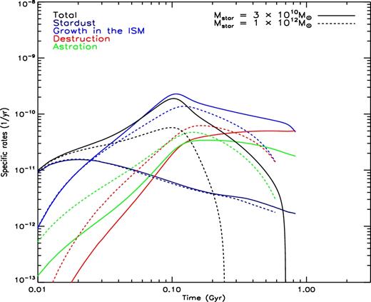
Theoretical specific dust production and destruction rates as a function of time in PSPHs. Results for two models of baryonic mass 3 × 10¹⁰ and 1012 M⊙ are shown (solid and dashed lines, respectively). In both cases, a standard Salpeter (1955) IMF is assumed. The green and red lines represent the destruction rates as due to astration and to shocks in SNe, respectively. The blue, dark blue and black lines represent the interstellar dust growth rates, the stellar dust production rates and the total rates, respectively.
Although the specific stellar dust production rates are comparable (dark blue solid and dashed lines), the lower mass model shows a lower specific destruction rate and a larger growth rate than the larger mass model. As shown in various previous studies (Dwek 1998; Calura et al. 2008, 2014; Pipino et al. 2011), the balance between destruction and growth is crucial to regulate the dust mass budget; in this case, we have shown the fundamental importance of these processes also in driving the DTS–Mstar relation.
5.2 Why a THIMF is needed
In models, larger dust masses can be achieved by means of a stellar IMF skewed towards massive stars, i.e. a THIMF, as this implies a more efficient stellar dust production (Gall et al. 2011b; Calura et al. 2014).
At the same time, even if the higher SN rates achieved with a THIMF imply larger destruction rates, also the accretion rate increases because of larger dust masses and of a lower dust-to-metal ratios (Calura et al. 2014). Moreover, the lower stellar masses achieved with a THIMF lead to dust masses produced per unit stellar mass larger than those obtained with a standard IMF.
Although no direct, ultimate proof for a different IMF in the early Universe or in starbursts can be found (Larson 1998; Elmegreen 2005; Narayan & Davé 2012), a THIMF offers a possible explanation for the large dust masses observed in high-z starbursts (Dwek et al. 2011; Gall et al. 2011a,b; Calura et al. 2014).
The study by Marks et al. (2012) suggests an IMF becoming more top-heavy at low metallicities and at high interstellar gas densities. Moreover, in principle, in extremely strong starbursts with SFR >1000 M⊙ yr−1, the formation of very massive and dense star clusters should be favoured, naturally leading to IMF skewed towards high-mass stars (Weidner, Kroupa & Pflamm-Altenburg 2011).
Possible ways to explore the IMF in starbursts include multiwavelength observations aimed at probing the production rate of ionizing photons. Recent results based on studies of unresolved stellar clusters in nearby galaxies show no deviation from a universal, standard IMF (Andrews et al. 2013). Future instruments such as the James Webb Space Telescope will allow one to extend such studies to higher redshifts, and this will be fundamental to gain more direct information on the IMF in distant, intense starbursts.
Finally, the study of interstellar metallicity offers another extremely efficient way to test the IMF in star-forming galaxies. In fact, as visible in Fig. 1, the interstellar metallicity achieved in PSPHs at the end of the starburst and calculated assuming a THIMF can be more than 0.5 dex higher than that computed with a Salpeter IMF.
The most dust-rich and strongly star-forming systems are expected to contain very large reservoir of metals. In such dust-enshrouded objects, metallicity diagnostics based on rest-frame optical emission lines are unreliable, as the optical spectral indices are likely unreliable (Santini et al. 2010). Currently, the Atacama Large Millimeter/submillimeter Array (ALMA) offers the possibility to overcome this problem. In fact, a recent ALMA study based on the flux ratio of the FIR fine-structure emission lines [N ii] 205 μm and [C ii] 158 μm as metallicity diagnostics has revealed high levels of chemical enrichment even in a starburst at z = 4.76 (Nagao et al. 2012).
6 CONCLUSIONS
In this paper, we have considered a few dust-related scaling relations in galaxies at both low and high redshift, in order to gain some basic information on how star formation has progressed in galaxies of various morphological types as a function of cosmic history. The scaling relations studied here include dust mass, gas mass, stellar mass and SFR.
We have assembled various data sets at various redshifts, and which include galaxies characterized by a large variety of star formation histories and spanning a large dynamical range in both stellar mass and SFR. These data sets include local spiral discs such as those from the SINGS and KINGFISH projects, as well as data from the COSMOS/GOODS surveys, which span a wide redshift range and include many intense starbursts, as well as local ULIRGs and of SMGs at z > 1.
The data sets have been interpreted by means of chemical evolution models of galaxies of different morphological types, useful in particular to set a few constraints on the star formation history of the observed systems and to understand which physical processes drive the relations considered in this paper.
We have focused in particular on the amount of dust per unit stellar mass observable in local and distant discs and starbursts, which represents a measure of the dust production efficiency or, rather, of the survival capability of dust grains in quiescent galaxies and in starbursts. We study how this quantity evolves as a function of the stellar mass and redshift, and how it can be theoretically accounted for.
Our main results can be summarized as follows.
The dust content of local disc galaxies and ULIRGs is broadly accounted for by our chemical evolution models for spirals and PSPHs, respectively. On the other hand, in several cases the large dust masses observed in some high-redshift samples are difficult to reproduce by means of our models with standard assumptions on basic parameters such as the stellar IMF. This fact outlines a notorious dust budget problem already addressed in previous studies (Dwek et al. 2007; Gall et al. 2011a; Mattsson 2011; Hjorth et al. 2014; Rowlands et al. 2014). A THIMF in PSPHs allows us to alleviate the tension between data and models. However, in a few particularly dust-rich systems, other processes could play an important role, such as an enhanced dust growth efficiency (Valiante et al. 2011; Asano et al. 2013; Nozawa et al. 2015).
The study of the relation between dust mass and SFR in high-redshift samples allows one to extend this diagram to SFR values larger than those measured in local starbursts. In high-redshift samples, the Mdust–SFR relation appears flatter than the one derived in local star-forming galaxies by da Cunha et al. (2010). In fact, the maximum dust masses observed in high-redshift samples are of the same order as those observed locally, but the SFRs of high-redshift systems are generally larger. The model results indicate that the two morphological types tend to occupy rather distinct regions of this diagram: spiral discs occupy the lowest dust mass, lowest SFR part, whereas PSPHs occupy the opposite part of the plot, characterized by the highest SFR and largest Mdust values. Overall, the samples considered in this work which bear information on the morphology of the galaxies tend to reflect this trend. In agreement with Hjorth et al. (2014), our models indicate that there is a maximum dust mass achievable in systems with log[SFR/(M⊙ yr−1)] > 3. Our models show the dependence of this ‘maximal dust mass’ on the star formation history of PSPHs and spirals. This quantity tends to increase as a function of the SFR and, in PSPHs, increases also at fixed SFR if one assumes a THIMF.
The Mdust–SFR and the Mdust–Mgas correlations are populated by starburst galaxies caught in their latest star-forming phases. The PSPH models show that after a rapid increase of the dust build-up, occurring at nearly constant SFR, the dust masses reach a maximum and then start decreasing with the SFR. During this late star-forming phase, each model moves along a nearly diagonal line which starts from the maximum of the dust mass ever achieved during the whole evolution, and evolves towards lower Mdust and Mgas values, i.e. towards the point which marks the end of star formation.
The observational data sets indicate an anti-correlation between the DTS and the stellar mass, implying that the production of dust per unit stellar mass is particularly efficient in low-mass galaxies. The theoretical models demonstrate the strong dependence of this quantity on the star formation history. In systems characterized by a nearly constant and prolonged star formation activity, the DTS shows a rather flat behaviour with respect to stellar mass. On the other hand, in the earliest phases of PSPHs, the DTS grows steeply up to a maximum DTS level, after which it experiences a decrease which extends up to the end of SF. Once again, our models computed with a standard IMF underestimate the DTS observed in distant starburst galaxies; the adoption of a THIMF helps reducing significantly the tension between data and models.
The decreasing trend of the DTS with stellar mass reflects the late starburst phase of PSPH models, i.e. the phase following the peak of the star formation epoch, characterized by a constant decrease of both the SFR and of the net rate of dust production.
In the mean time, the continuous increase of the stellar mass causes the DTS to proceed along a diagonal line towards the end of star formation.
The DTS ratio is larger in low-mass PSPHs because these are characterized both by a lower specific destruction rate and by a larger specific growth rate than the larger mass models.
The observed DTS ratio shows an increasing trend with redshift in the range 0 ≤ z ≲ 2.5. It increases roughly by 0.5–0.7 dex from z ∼ 0 to z ∼ 1, to reach a plateau in the interval 1 ≤ z ≤ 2. The values computed for the detections of the sample at z ∼ 6 are within the error bars to those of SMGs. However, at z ≳ 6, the spread in the DTS is expected to be wide. Our models predict that at some point at larger redshift, the global DTS is expected to decrease with increasing redshift. The growth of dust in the early Universe could be extremely rapid (Mattsson 2016), as supported also by the few notable cases of dust-free galaxies found at z > 6.5 (Ouchi et al. 2013; Inoue et al. 2016).
The average DTS computed from the data of local discs and ULIRGs are comparable with theoretical estimates for spiral galaxy models and PSPHs, respectively. Some of the observational estimates at z > 1 are reproduced by our PSPH models which adopt a THIMF. This could be another indication that a THIMF is required to explain the large dust masses in high-redshift data. However, such an assumption leads to metallicities larger than the ones computed with a standard IMF by more than 0.5 dex. Future IR studies based on the analysis of flux ratio of fine-structure emission lines as metallicity indicators (Nagao et al. 2012) will shed light on the metal content of high-z starbursts.
In general, a better understanding of the grain size distribution and temperatures, as well as their composition, will be fundamental in order to improve the accuracy in observational estimates of the dust mass. In particular, a valuable quantity useful to constrain the size distribution is the extinction curve, which depends also on the dust chemical composition. In principle, the study of the extinction curves in galaxies whose chemical abundance pattern can be derived by means of different observables, such as in the Milky Way or in the Small Magellanic Cloud, can be very useful to constrain the size distribution (e.g. Schurer et al. 2009).
On the theoretical side, it will be important to match the predictions from chemical evolution models including dust production to spectrophotometric codes such as grasil (Silva et al. 1998); previous efforts in this direction are those of Schurer et al. (2009) and Pozzi et al. (2015). In this regard, significantly new perspectives are also offered by the grasil-3d tool (Domínguez-Tenreiro et al. 2014), designed to match a detailed spectrophotometric modelling of dust, including radiative transfer effects, to the outputs of hydrodynamical galaxy formation codes.
Another future step will be to investigate the evolution of the dust content in galaxies by means of models computed within a cosmological framework. An attempt to model dust production in a fully cosmological context was made by McKinnon et al. (2016), which provides detailed three-dimensional theoretical distributions of the dust in simulated galaxies. However, the best tools to provide a cosmology-based, theoretical description of the global properties of galaxies are semi-analytic models (SAMs) of galactic evolution. Ideally, in order to extend their predictive power to dust-related properties, next-generation SAMs will have to include a detailed treatment of the chemical evolution of refractory elements (e.g. Calura & Menci 2009, 2011), of dust creation and destruction (e.g. Valiante et al. 2014) as well as a spectrophotometric treatment of dust grains.
Acknowledgments
We thank the anonymous referee for valuable suggestions which improved the quality of our work. Loretta Dunne is acknowledged for interesting discussions. PS acknowledges financial support from the European Union's Seventh Framework Programme ASTRODEEP (FP7/2007- 2013), grant agreement no. 312725.
For the conversion of the observed stellar masses from a Salpeter to a Larson (1998) THIMF with mc = 10 M⊙, Hjorth et al. (2014) suggest a rescaling downwards by a factor of ∼3, corresponding to −0.48 dex in logarithm (see also Dwek et al. 2011). In our case, we assume a considerably less extreme IMF characterized by mc = 1.2 M⊙; hence, such a conversion should be regarded as an upper limit. In our case, a reasonable conversion is likely to be of 0.1–0.2 dex. Given the large dynamic range of stellar masses characterizing the models and the data in this work, which spans from ∼106 to 1012 M⊙, in our analysis we ignore such a conversion.
