


Abstract
Energy losses from isolated neutron stars are commonly attributed to the emission of electromagnetic radiation from a rotating point-like magnetic dipole in vacuum. This emission mechanism predicts a braking index n = 3, which is not observed in highly magnetized neutron stars. Despite this fact, the assumptions of a dipole field and rapid early rotation are often assumed a priori, typically causing a discrepancy between the characteristic age and the associated supernova remnant (SNR) age. We focus on neutron stars with ‘anomalous’ magnetic fields that have established SNR associations and known ages. Anomalous X-ray pulsars (AXPs) and soft gamma repeaters (SGRs) are usually described in terms of the magnetar model that posits a large magnetic field established by dynamo action. The high magnetic field pulsars (HBPs) have extremely large magnetic fields just above quantum electrodynamics scale (but below that of the AXPs and SGRs), and central compact objects (CCOs) may have buried fields that will emerge in the future as nascent magnetars. In the first part of this series, we examined magnetic field growth as a method of uniting the CCOs with HBPs and X-ray dim isolated neutron stars (XDINSs) through evolution. In this work, we constrain the characteristic age of these neutron stars using the related SNR age for a variety of energy-loss mechanisms and allowing for arbitrary initial spin periods. In addition to the SNR age, we also use the observed braking indices and X-ray luminosities to constrain the models.
1 INTRODUCTION
In previous work (Rogers & Safi-Harb 2016, hereafter RSH16), we studied a parametrized phenomenological model for describing magnetic field growth in neutron star (NS) evolution. Assuming that the external dipole field is buried by an intense process of fall-back accretion after the formation of the NS (Muslimov & Page 1995, 1996), the slow diffusion from the stellar surface exerts a time-dependent torque on the NS (Geppert, Page & Zannias 1999). This process may provide an explanation for the observed braking indices of young pulsars with n ≠ 3 (Espinoza 2012; Archibald et al. 2016), in contrast to the prediction of a rotating magnetic dipole in vacuum (n = 3; Ostriker & Gunn 1969). Magnetic field growth provides an evolutionary link between apparently disparate classes of NS, such as the extremely weak field1 subset of NSs known as central compact objects (CCOs), high magnetic field pulsars (HBPs) and the X-ray dim isolated NSs (XDINSs). On the other hand, magnetic field decay has been invoked to describe the evolution of the anomalous X-ray pulsars (AXPs) and soft gamma repeaters (SGRs). These objects are conventionally described by the magnetar model that posits the development of large magnetic fields via dynamo action from rapid rotation early in the life of the NS, necessary to support the core of the massive progenitor from collapse (Duncan & Thompson 1992; Akiyama et al. 2003; Thompson, Quataert & Burrows 2005). However, the distinction between the apparently rotation-powered HBPs, with dipole fields just above the quantum critical limit, BQED = 4.4 × 10¹³ G, and the magnetically powered AXPs and SGRs (B ≥ BQED) is significantly blurred after the HBPs were observed displaying magnetar-like activity (Gavriil et al. 2008; Kumar & Safi-Harb 2008; Göğüs et al. 2016), and radio emission was observed from magnetars (Camilo et al. 2007). Moreover, the SNRs associated with the AXPs and SGRs show evidence of ‘typical’ explosion energies (≤1051 erg) and not superenergetic as one would expect from a rapidly rotating proto-NS (Vink & Kuiper 2006; Kumar, Safi-Harb & Gonzalez 2012; Safi-Harb & Kumar 2013; Kumar et al. 2014). These complications are difficult to reconcile with the standard magnetar picture.
The SNR association can also impose a profound constraint on the NS energy loss, since the NS characteristic age τ must agree with the age of the associated SNR τSNR± (denoting the lower SNR age with a minus and the upper limit with a plus). Generally the errors on SNR ages are large, and depend sensitively on both the distance to the remnant and its expansion velocity or assumed phase of evolution. Despite these large error bars, poor agreement is generally still found with the NS characteristic age, in some cases by orders of magnitude. The CCOs present extreme examples of this dichotomy. These objects appear to be extremely old NSs, but they are intrinsically young, being associated with young SNRs.
The discrepancy between NS and SNR age has been recently studied by several authors (e.g. Popov & Turolla 2012; Gao et al. 2014; Nakano et al. 2015, RSH16). Popov & Turolla (2012) calculate the initial spin period P0 as a function of SNR age and constant braking index for a set of 30 radio pulsars associated with SNRs. Gao et al. (2014, 2016) address the magnetar–SNR associations, however they include uncertain associations, SNRs with uncertain or unknown ages, and assume that P0 ≪ P. Nakano et al. (2015) explain the large discrepancy between the age of SNR CTB 109 and its AXP 1E 2259+586 by magnetic field decay, however, they also assume a very small initial spin period. In this work, we explore the relationship between NS and SNR ages for a selection of energy-loss mechanisms with arbitrary initial period P0, using the measured NS properties (period P, period derivative |$\dot{P}$|, braking index n and X-ray luminosity Lx). The properties of the secure NS–SNR pairs considered in this work are summarized in Table 1. The SNR ages and distance estimates were collected from the University of Manitoba's high-energy catalogue of SNRs, SNRcat2 (Ferrand & Safi-Harb 2012), while the McGill pulsar catalogue3 (Olausen & Kaspi 2014) provides the properties of the AXPs and SGRs. In Section 2, we discuss the general expression relating a constant braking index and initial spin period for power-law torques. Section 2.2 introduces time-dependent magnetic fields and describes magnetic field evolution. We discuss braking by the emission of relativistic winds in Section 2.3. We provide further discussion of our results in Section 3 and summarize our conclusions in Section 4. Justification for excluding some of the NS–SNR pairs is discussed in the Appendix.
For a given PSR, P is the period, |$\dot{P}$| the period derivative, and Lx the X-ray luminosity in the range 2–10 keV from the McGill magnetar catalogue (http://www.physics.mcgill.ca/∼pulsar/magnetar/main.html). The equatorial magnetic field strength in flat space–time is B0. The NS characteristic age is τPSR and the SNR age limits are τSNR− and τSNR+. The SNR ages have been compiled in the U. of Manitoba's SNR Catalogue (SNRcat, Ferrand & Safi-Harb 2012, http://www.physics.umanitoba.ca/snr/SNRcat/). References to SNR ages in this table are [1]: Kumar et al. (2014), [2]: Nakano et al. (2015), [3]: Nakamura et al. (2009), [4]: Park et al. (2012), [5]: Corbel et al. (1999), [6]: Kumar et al. (2012), [7]: Gotthelf et al. (2000), [8]: Becker et al. (2000), [9]: Zavlin et al. (2000), [10]: Sun et al. (2004). References to the braking indices included here are [11]: Weltevrede et al. (2011), [12]: Livingstone et al. (2006), [13]: Livingstone et al. (2011).
| Observed properties of AXPs, SGRs, HBPs, and CCOs associated with SNRs | ||||||||||
| PSR | P | |$\dot{P}$| | n | Lx | |$\dot{E}$| | τPSR | B0 | SNR | τSNR− | τSNR+ |
| s | 10−11ss−1 | 1033 erg s−1 | 1033 erg s−1 | kyr | 1014 G | kyr | kyr | |||
| AXP 1E 1841–045 | 11.79 | 4.09 | 184 | 0.99 | 4.75 | 7.05 | G27.4+0.0 (Kes 73) | 0.75 | 2.1 [1] | |
| AXP 1E 2259+586 | 6.98 | 4.8e − 2 | 17 | 5.3e − 2 | 228.317 | 0.59 | G109.1-01.0 (CTB 109) | 10 | 16 [2] | |
| CXOU J171405.7–381031 | 3.83 | 6.40 | 56 | 45.14 | 0.95 | 5.0 | G348.7+00.3 | 0.35 | 3.15 [3] | |
| SGR 0526–66 | 8.05 | 3.8 | 189 | 2.87 | 3.358 | 5.60 | N49 | – | 4.8 [4] | |
| SGR 1627–41 | 2.59 | 1.9 | 3.6 | 33.9 | 2.164 | 2.25 | G337.3–0.1 | – | 5.0 [5] | |
| PSR J1119–6127 | 0.408 | 0.40 | 2.684 ± 0.002 [11] | 2.4 | 2325 | 1.616 | 0.41 | G292.2–0.5 | 4.2 | 7.1 [6] |
| PSR J1846–0258 A | 0.325 | 0.71 | 2.64 ± 0.01 [12] | 20.0 | 8161 | 0.726 | 0.485 | G029.7–0.3 (Kes 75) | 0.430 | 4.3 [7] |
| PSR J1846–0258 B | 0.327 | 0.71 | 2.16 ± 0.13 [13] | 8056 | 0.728 | 0.49 | ||||
| RX J0822.0–4300 | 0.112 | 8.3e − 4 | 5.6 | 233 | 213.799 | 9.80e − 4 | G260.4–3.4 (Puppis A) | 3.70 | 5.20 [8] | |
| 1E 1207.4–5209 | 0.424 | 2.23e − 6 | 2.50 | 1.16e − 2 | 3.01e5 | 9.85e − 4 | G296.5 +10.0 (PKS 1209–51/52) | 2.0 | 20.0 [9] | |
| CXOU J185238.6+004020 | 0.105 | 8.68e − 7 | 5.30 | 0.296 | 1.92e5 | 3.06e-4 | G033.6+00.1 (Kes 79) | 5.4 | 7.5 [10] | |
2 BRAKING MECHANISMS
2.1 Power-law torques
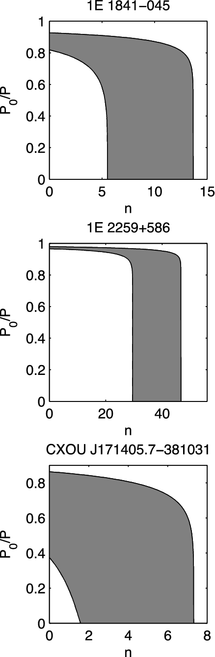
Power-law age constraints for the AXPs: 1E 1841–045, 1E 2259+586, and CXOU J171405.7–381031. Grey areas indicate regions where the pulsars’ ages agree with the SNR age estimates (see Table 1). We show that large ratios of initial and observed spin periods are needed for a large range of braking indices using a power-law spin-down torque.
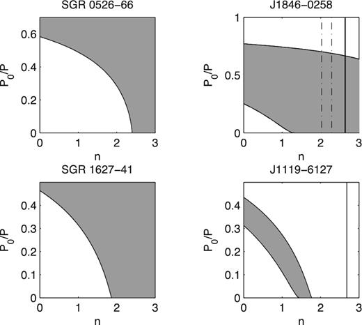
Power-law age constraints. Left column: SGRs 0526–66 (top) and 1627–41 (bottom). Right column: HBPs J1846–0258 (top) and J1119–6127 (bottom). See Table 1 and text for details. The vertical lines included in the plots of the HBPs mark the measured braking indices including uncertainties. The pre-outburst and post-outburst braking indices of HBP J1846–0256 are shown by the solid and dash–dotted lines, respectively.
The CCOs are not plotted in these figures as they require large initial spin periods (P0 > 0.99P) for braking index in the range 0 < n < 50. These large initial spin periods are insufficient to generate a strong dynamo and imply a weak magnetic field. This scenario forms the basis of the proposed ‘anti-magnetar’ model of CCOs, which posits an extremely weak field orders of magnitude lower than the magnetar model and X-ray luminosity due to thermal emission from residual cooling (Gotthelf & Halpern 2009; Gotthelf, Halpern & Alford 2013), though the CCO 1E 16348-5055, associated with the SNR RCW 103, has been observed to display magnetar-like bursting behaviour (D'Ai et al. 2016; Rea et al. 2016). The constant braking index assumption with the observed SNR age constraints naturally leads to this view since P0 ≈ P is naturally recovered. However, when more complex evolutionary scenarios are considered, this condition can be alleviated, leading to alternatives to the high P0/P ratios of the CCOs. Note that the SGRs in Fig. 2 have no lower SNR age estimates and so are only gently constrained.
Systems with a measured braking index provide interesting examples with further constraints. The HBP J1119–614 associated with the SNR G292.2–0.5 has n = 2.684 ± 0.002 (Weltevrede, Johnston & Espinoza 2011). However, in order for the pulsar to have an age that is consistent with the SNR, we expect the braking index to be much lower than this value. As shown in Fig. 2, we find that the braking index is constrained by the SNR's age to be 1.45 < n < 1.8 provided P0 ≪ P, consistent with an earlier estimate n < 2 (Kumar et al. 2012). We use the period, period derivative and braking index determined by Weltevrede et al. (2011), however we note that Antonopoulou et al. (2015) have a measured value n = 2.677, which does not follow from the spin parameters in that work due to the details of the analysis performed. The small difference between the two braking indices will not significantly affect the results. The HBP J1846–0258 demonstrates that the braking index varied over time. Measurements of the spin period and derivatives were made before and after a magnetar-like outburst detected in 2006 (Livingstone et al. 2006; Gavriil et al. 2008; Kumar & Safi-Harb 2008), and show changes in the pre- and post-outburst braking index. We include both in Fig. 2, with the measurements made from 2000 to 2003 (n = 2.64 ± 0.01; Livingstone et al. 2006) and 2008–2010 (n = 2.16 ± 0.13; Livingstone et al. 2011). The braking index has remained at comparatively low values (Archibald et al. 2015). The physics leading to the constancy of the X-ray luminosity and pulse profile from the pre- to post-outburst phase is difficult to explain in most conventional models. Whether the braking index will eventually return to the pre-outburst value remains an open question. Monitoring this object is crucial to address this question.
2.2 Magnetic field evolution
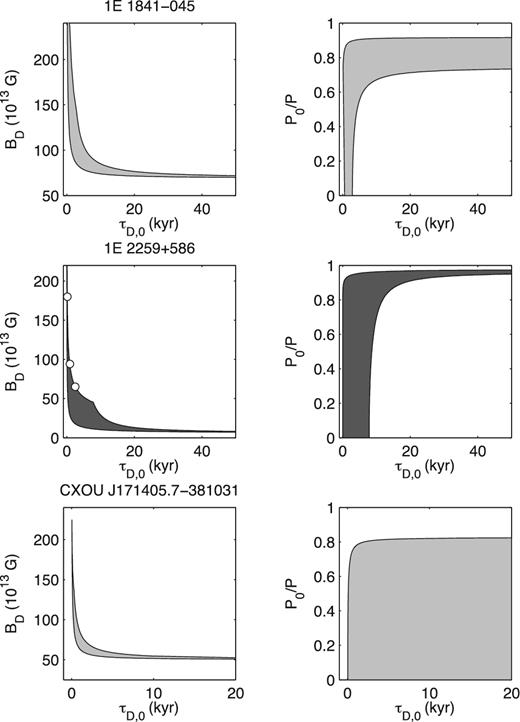
Field decay age constraints for the AXPs 1E 1841–045 (top row), 1E 2259+586 (middle row) and CXOU J171405.7– 381031 (bottom row). In the left column, we plot the initial field BD in units of 1013 G versus the initial decay time-scale τD,0 in kyr, and in the right column, we plot the initial period fraction P0/P against the time-scale. These parameter space regions are calculated for a variety of α between 0 and 2. Solutions that satisfy the SNR age constraints are shown as the shaded regions. Light grey indicates decay models that are capable of accommodating the observed X-ray luminosity. The solutions for 1E 2259+586 reported by Nakano et al. (2015) are plotted as the white discs on the BD − τD,0 plot. These solutions have P0 = 3 ms, so occupy the region near the τD,0 axis and are not shown on the associated right-hand panel.
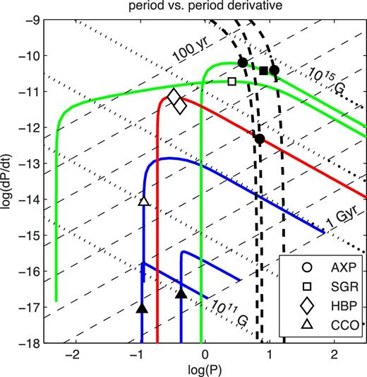
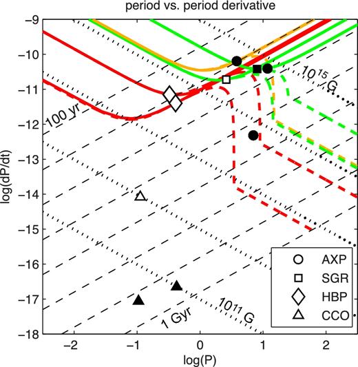
Period versus period derivative. Lines of constant characteristic age are plotted as the dashed lines ranging from 100 yr (upper left) to 1 Gyr (lower right), increasing by factors of 10. Lines of constant magnetic field are plotted as the dashed lines from 1011 G (lower right) to 1015 G (upper left), increasing by factors of 10. AXPs are plotted as circles and have dashed evolutionary trajectories given by field decay. The SGRs are squares and have green field growth trajectories. HBPs are diamonds and the J1846–0258 field growth path is plotted in red. Note that we do not provide a trajectory for HBP J1119–6127 (see text for details). Finally, the CCOs are triangles with field growth paths shown in blue. Sources with |$L_{\rm x}<\dot{E}$| are hollow and sources with |$L_{\rm x}>\dot{E}$| are filled. Both axes are plotted on logarithmic scales.
We also performed a joint fit for the AXPs and fit the observed spread of τPSR and τSNR± in terms of 1E 2259+586 since it has the largest characteristic age among the AXPs. In this view, the age discrepancy is an evolutionary effect. The relationship between τPSR and τSNR± for all systems in Table 1 is plotted in Fig. 5. This figure also includes the τPSR = τSNR line, shown in heavy black. Since we consider general initial spin periods in our models, our parameter sets include the solutions found by Nakano et al. (2015), who assumed a constant P0 ≪ P. The Nakano et al. (2015) solutions are marked as dashed black lines, and have α values 0.60, 1.00 and 1.40, where Colpi et al. (2000) favour α = 1. Our joint fits occupy the light grey region in Fig. 5. Following this approach, we also consider a joint fit to the CCOs in terms of CXOU J185238.6+004020. The only viable field decay mode for the CCOs requires exponential decay since the characteristic ages are so long for these objects. Since exponential decay is disfavoured among magnetic field decay modes (Dall'Osso et al. 2012; Nakano et al. 2015), this result suggests that field decay is unlikely to properly describe the CCO evolution, which we suggest is more neatly accommodated by field growth (RSH16). The parameters that describe the joint fit are given in Table 2.
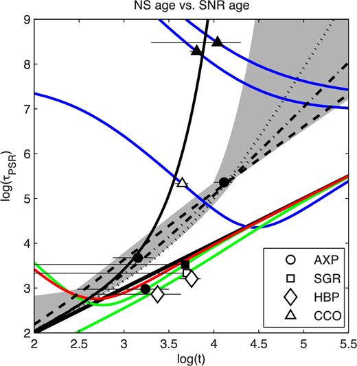
Pulsar age versus SNR age. The horizontal lines show the spread in SNR age estimates, ranging from τSNR − to τSNR+ (see Table 1). If one of these limits is not available, we plot the error bar to the corresponding axis limit. AXPs are plotted as circles, SGRs are squares, HBPs are diamonds and CCOs triangles. Sources with |$L_{\rm x}<\dot{E}$| are not filled, and sources with |$L_{\rm x}>\dot{E}$| are filled. Each of the axes are plotted on a logarithmic scale. The diagonal black line corresponds to τ = t. The light grey region is our joint fit region for field decay. The solutions found by Nakano et al. (2015) are plotted as the heavy dashed (α = 0.6), dash–dotted (α = 1.0) and dotted (α = 1.4) lines. The heavy solid black line is our best joint-fit solution found for the CCOs. The details of these solutions are given in Table 2. Note that we do not provide a trajectory for HBP J1119–6127.
| Solutions shown in Fig. 5 | ||||||
| Joint field decay | ||||||
| Object | α | – | τD,0 (yr) | BD,0 (×1013 G) | P0 (ms) | – |
| AXP | 0.60 | 2500 | 65.00 | 3.0 | ||
| AXP | 1.00 | 920 | 94.00 | 3.0 | ||
| AXP | 1.40 | 160 | 180.00 | 3.0 | ||
| CCO | 0.00 | 1180 | 3.48 | 421.00 | ||
| Individual field growth | ||||||
| Object | α | ε (×10−5) | τG (yr) | BG (×1013 G) | P0 (ms) | t (kyr) |
| SGR 0526–66 | 0.155 | 0.007 | 789.730 | 57.581 | 0.868 | 4.800 |
| SGR 1627–41 | 0.319 | 2.023 | 3700.000 | 41.763 | 0.005 | 5.000 |
| HBP J1846–0258 A | 0.000 | 6.372 | 252.686 | 5.178 | 0.182 | 0.900 |
| HBP J1846–0258 B | 0.341 | 5.487 | 223.731 | 6.014 | 0.182 | 0.900 |
| CCO RX J0822.0–4300 | 0.202 | 818.016 | 33550.160 | 0.909 | 0.112 | 4.450 |
| CCO 1E 1207.4–5200 | 0.700 | 100 | 98245.295 | 0.045 | 0.423 | 11.000 |
| CCO CXOU J185238.6+004020 | 0.468 | 0.017 | 12483.740 | 0.014 | 0.105 | 6.450 |
For the HBP J1119–6127, we were unable to find a braking index in the observed range given the age limits of the associated SNR, G292.2–0.5 (Kumar et al. 2012), and found a value n ≈ 1.2 (RSH16). This differs significantly from the measured braking index, n = 2.684 ± 0.002. As an alternative, we have also fit J1119–6127 by searching for solutions that satisfy the braking index constraint and determining the resulting age. This approach gives a maximum model age tSNR ≈ 1.76 kyr for n in the observed range, well short of the 4.2 kyr lower SNR age limit for G292.2–0.5. Due to these discrepancies with observation we do not show a trajectory for HBP J1119–6127 in Figs 4 and 5.
2.3 Braking by relativistic wind
In general, the Hall time-scale for magnetic field evolution depends on the strength of the magnetic field, as seen in equation (4). For young NSs with fields below 1014 G, this time-scale may be longer than the observed SNR age. Therefore, magnetic field growth does not have a dramatic effect on these young NSs. However, many of these systems are observed to have a braking index n < 3 (Espinoza 2012; Archibald et al. 2016). A possible explanation for these low braking indices may be through the emission of a relativistic particle wind (Thompson & Blaes 1998; Harding, Contopoulos & Kazanas 1999; Tong et al. 2013). However, the conclusive detection of wind nebulae around magnetars in particular is challenging due to the presence of dust-scattering haloes that accompany these X-ray bright, heavily absorbed objects (Esposito et al. 2013; Safi-Harb 2013). Only a handful of such nebulae have been proposed to be associated with highly magnetized NSs. For example, a wind nebula has been proposed to surround the magnetar Swift J1834.9–0846 in W41 (Younes et al. 2016), and the luminosity of a particle wind was estimated for SGR 1806–20 based on the X-ray and radio observations of the wind-powered nebula G10.0–0.3 (Thompson & Duncan 1996; Marsden, Rothschild & Lingenfelter 1999; Gaensler et al. 2005). In the pulsar wind model, relativistic particles load the magnetosphere with charge and distort the dipole field at large scales outside of the light cylinder. Besides affecting the NS spin-down, the emission of a relativistic wind can also offer an explanation for the significant timing noise that generally affects magnetar observations (Tsang & Konstantinos 2013). The HBPs J1119–6127 and J1846–0258 are clearly associated with pulsar wind nebulae (Gavriil et al. 2008; Kumar & Safi-Harb 2008; Ng et al. 2008; Safi-Harb & Kumar 2008; Safi-Harb 2013), suggesting that particle wind emission should play an important role in their evolution. We also expect that AXP and SGR evolution may be affected by wind emission due to candidate wind nebulae, but do not consider these models for the CCOs that do not show any evidence of PWN. However, we note that braking exclusively due to a steady particle wind produces a torque with a braking index n = 1, too low for the NSs with secure SNR associations in Table 1.
Period versus period derivative for wind models applied to systems with confirmed or candidate wind nebulae. Solid lines show the magnetar wind model, and dashed lines show the analogous VG(CR) model, with the effect of pulsar death included. Red lines are the evolutionary trajectories of the HBPs, green lines the SGRs and orange for the AXP CXOU J171405.7–381031. All other details are as in Fig. 4.
The luminosity and duty cycle parameters for the HBPs are plotted in Fig. 7. This figure shows the region of the Lp − Dp parameter space that satisfies the age constraint of J1846–0258 in the top panel, and J1119–6127 in the bottom panel. The pre-outburst and post-outburst constraints are plotted as dark grey and light grey, respectively. The changing braking index of J1846–0258 after the 2008 burst event requires a time-varying luminosity, but since no significant change in the X-ray pulse profile occurred any such change is strongly constrained (Archibald et al. 2015). We assume the derivative is negligible before and has a finite value after the burst, episodically varying about the mean on long time-scales. The braking index is calculated by fitting the pre-outburst state without a derivative term, and then solving for the required instantaneous derivative |$\dot{L}_{\rm p}$| from equation (22). An upper limit on the duty cycle exists from the condition that the wind luminosity must equal or exceed the X-ray luminosity. A minimum luminosity of Lp = Lx = 2 × 1034 erg s−1 with Dp < 0.947 (θ = 14|$_{.}^{\circ}$|08) using an initial period of 3 ms gives an SNR age of 805 yr. This solution requires dLp/dt = 2.82 × 1024 erg s−2, implying that even a relatively small luminosity growth rate after the glitch event has significant impact on the braking index. To compare with the results of previous studies that used the VG(CR) model, we fixed the inclination angle at θ = π/4 as used in Kou et al. (2016). At this inclination we find a polar magnetic field ∼1.25 × 10¹⁴ G, density factor κ between 56 and 59 growing at a rate |$2.55 \times 10^{-9} \le \dot{\kappa } \le 4.63 \times 10^{-9}$|. These values are similar to the results of Kou et al. (2016) after adjusting for the extra factor of 1/2, omitted by convention in that study, and using n = 2.19 (Archibald et al. 2015). The duty cycle Dp (or the corresponding inclination angle) strongly affects the solution, so knowledge of the system geometry is crucial to improve the results.
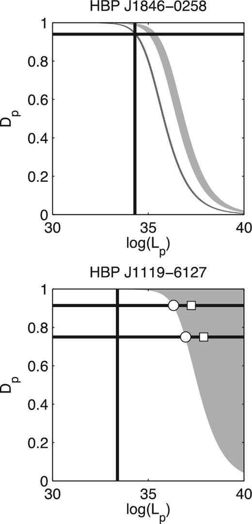
Dipole and wind age parameters for the HBPs J1846–0258 (top) and J1119–6127 (bottom). We plot the particle luminosity Lp against the duty cycle Dp. In the upper panel, the pre- and post-outburst phases of J1846–0258 are shown in dark and light grey, respectively. The horizontal line indicates the duty cycle limit at which Lp = Lx (vertical line). In the lower panel, parameters satisfying the SNR age are in the grey region. The parameters for four solutions with variable luminosity discussed in the text are plotted as dots (low SNR age) and squares (high SNR age) for an initial spin period of 3 ms. The X-ray luminosity Lx is marked with the vertical black line, and the limits on the inclination angle (duty cycle) are shown as the black horizontal lines.
As mentioned in Section 2.2, the braking index for J1119–6127 with a constant luminosity produces a braking index that is smaller than observed (n ∼ 1.2) when using the 4.2–7.1 kyr age range of G292.2–0.5, though the age is matched well. Conversely, a constant braking index with the contouring approach gives solutions up to a maximum age of tSNR ≈ 1.76 kyr. This result is similar to the prediction of the field growth model (Section 2.2). This problem vanishes when using of a wind model with a variable luminosity. The region of parameter space with acceptable solutions for J1119–6127 is shown on the lower panel of Fig. 7 as a light grey area and requires a decreasing luminosity |$\dot{L_{\rm p}}<0$| that gives a lower braking index in the recent past as suggested by Kumar et al. (2012). The inclination angle of J1119–6127 has been determined to be in the range 17° ≤ θ ≤ 30° (Weltevrede et al. 2011), and the corresponding duty cycle is then between 0.91 and 0.75, respectively. These limits are plotted as the horizontal lines in Fig. 7. To set limits on the parameters, we consider an initial period of 3 ms at the duty cycle extremes for the minimum and maximum SNR age, plotted as discs and squares, respectively. This gives luminosity between 2.04 × 1036 and 7.72 × 1037 erg s−1, with time derivative between −2.54 × 1027 and −6.61 × 1025 erg s−2.
3 DISCUSSION
We account for the X-ray luminosity of the AXPs using a decaying field, except for the AXP 1E 2259+586. For this system field decay was insufficient to explain the luminosity by a factor between 2 and 20. This discrepancy was found in previous work (Dall'Osso et al. 2012) and led to the suggestion of an additional internal decaying toroidal field component.
The joint fits for the decaying field in Fig. 5 also provide some interesting suggestions. The error bar on the age of the remnant G348.7+00.3, associated with AXP CXOU J171405.7–381031, is large and crosses the line for which τPSR = τSNR. If CXOU J171405.7–381031 is like the other AXPs then the NS characteristic age should appear older than the SNR and it has a braking index n > 3. In this case, the joint fit for field decay unites the AXPs as snapshots in the evolution of these objects. If the converse is true, the remnant appears older than the AXP and the braking index is n < 3, implying that field decay is the wrong explanation for this behaviour, so some other mechanism must influence the behaviour of the NS. These comments also apply to the SGRs that do not have conclusive lower SNR age limits, and from this perspective it is not clear if these sources evolve by field growth or decay. The AXP CXOU J171405.7–381031 and the SGRs 0526–66 and 1627–41 are similar in that they all have a τPSR < τSNR+, and there is no distinct age discrepancy. Since no lower age estimates for N49 or G337.3–0.1 exist, the SGR parameters cannot be tightly constrained in model fitting. In order to gain more insight on these systems, it is critical to tighten the age estimates of the associated SNRs, and future measurements of the braking index (whenever possible) would conclusively settle this issue.
Both HBPs provide extremely interesting insights on energy-loss mechanisms. The HBP J1119–6127 shows a faint wind nebula that is very similar in characteristics (e.g. |$L_{\rm x}/\dot{E}$| and photon index) to wind nebulae surrounding rotation-powered pulsars (Safi-Harb & Kumar 2008). Our study confirms these expectations and shows a changing particle luminosity is needed for this system. We find the required instantaneous luminosity derivative, but more detailed scenarios have been discussed in the literature (see for example, Tong et al. 2013).
Variability in the wind nebula around HBP J1846–0258 has been observed in reaction to outburst activity of the NS (Ng et al. 2008). The wind emission mechanism can account for both pre- and post-burst states with the age and braking index constraints with a varying particle luminosity. Archibald et al. (2015) argue against the applicability of the wind-braking mechanism in HBP J1846–0258, and favour an explanation based on changes in the structure of the magnetosphere. However, Kou et al. (2016) have explained the difference in terms of a time-dependent wind density, which our work supports. Kou et al. (2016) argue that the necessary wind density enhancement is on the order of ∼1 per cent, which provides a small change to the observed luminosity but is significant enough to explain the observed change in braking index. We also provide a link between the various wind models such as the magnetar wind model presented in Harding et al. (1999) and the various forms of acceleration gap models used in the literature (Xu & Qiao 2001).
In general, the dependence of the Hall drift time-scale on the magnetic field (equation 4) determines the physics at work in describing NS evolution. Pons et al. (2012) has analysed the properties of a sample of 118 NSs, most of which are recycled millisecond PSRs with measured braking index and relatively low magnetic fields. Their fig. 2 shows the evolutionary properties of this sample of low-field NSs. A number of conclusions are drawn based on this population, namely that the objects transition from an initial state with braking indices n < 3 at early times to n > 3 from field decay on Ohmic time-scales between 10 and 100 kyr. Moreover, Pons et al. (2012) also show the results of simulations that use all possible decay modes of the magnetic field including both Hall drift and Ohmic dissipation, along with an early period of accretion to bury the magnetic field. The evolutionary trajectories for submerged fields shown in Fig. 4 reproduce the qualitative behaviour from the simulations for a substantial amount of accreted mass ≈10−3 M⊙. This scenario produces a vertical trajectory in P and dP/dt at early times. However, simulations with a shallow submerged field under lower accreted mass (≈10−5 to 10−4) nearly follow along lines of constant magnetic field, relevant for the HBPs. The simulations presented in Pons et al. (2012) predict that the braking indices of the HBPs will be mainly affected by field decay and should generally increase with time. Pons et al. (2012) also provide several examples of additional, potentially dominant, effects such as alignment of the magnetic field and magnetospheric variability. Since the environs surrounding the young high-field PSRs are complex and display wind nebulae (Safi-Harb & Kumar 2008; Safi-Harb 2013; Younes et al. 2016), short-time-scale variations due to the emission of particle winds should also be included as an evolutionary effect significant for the variation of braking index and spin. The evolutionary tracks in Fig. 6 for wind emission predict that the braking index should decrease steadily with time, however the variable nature of the wind luminosity needed to explain the post-outburst braking index of J1846–0258 argues against such an orderly evolution. Realistically, both magnetothermal and particle wind effects must play important roles in the behaviour of the HBPs.
4 CONCLUSIONS
We have analysed several mechanisms to produce the spin evolution of ‘anomalously’ magnetized NSs by studying energy-loss mechanisms constraining the NS characteristic age and SNR age to agree. We also use the X-ray luminosity and braking index constraints when available. For constant values of the braking index, we find a large ratio of P0/P is often required to satisfy the age constraints, at odds with the prediction of the magnetar model. This leads to a discussion of emission mechanisms in which the braking index is time dependent.
For the AXPs, which have τPSR > τSNR±, we favour the field decay scenario that predicts n > 3, and we explored the properties of these solutions in terms of NS evolution. We performed a joint fit to the AXPs simultaneously and found a family of solutions containing those previously studied by Nakano et al. (2015). The CCOs require exponential decay to explain their joint behaviour, which is an unlikely decay mode for physical reasons. However, the population of CCOs can be neatly described in terms of field growth, which links apparently disparate classes of NS by evolution. This provides an evolutionary link between NSs in the HBP and CCO regions of the |$P-\dot{P}$| phase diagram (Ho 2015, RSH16). Despite the success of field growth in isolated NSs, the two HBPs that are associated with wind nebulae inside SNRs are best described in terms of a wind model (Harding et al. 1999; Tong et al. 2013; Kou et al. 2016). The wind model was able to account for the J1846–2058 pre- and post-outburst braking index, remnant age and X-ray luminosity but requires a variable particle luminosity. In our analysis, we relate the magnetar wind and acceleration gap models and show they describe the same qualitative evolutionary trajectories through the |$P-\dot{P}$| phase space, despite the unique physical assumptions included in each scenario.
Constraining the SNR ages will produce tighter constraints on the parameters for each of the models considered in this work. Finally, increasing the sample of pulsar–SNR secure associations and improving the age, distance estimates and braking indices are crucial to expand on this study.
Acknowledgments
This work was primarily supported by the Natural Sciences and Engineering Research Council of Canada (NSERC) through the Canada Research Chairs Program. SSH also acknowledges support by an NSERC Discovery grant and the Canadian Space Agency. This research made use of NASA's Astrophysics Data System, McGill's magnetars catalogue and the U. of Manitoba's high-energy SNR catalogue (SNRcat). We thank Harsha Kumar for discussions on magnetar SNRs and Gilles Ferrand for contributions to SNRcat. We also extend thanks to the anonymous referee for providing a valuable review which improved the overall quality of the text.
In this work, we use the dipole magnetic field at the stellar equator and poles, denoted with subscripts eq and p, respectively, and defined as |$B_{{\rm eq}}=3.2 \times 10^{19}\sqrt{ P \dot{P} }$| (G) and Bp = 2Beq. The field is inferred from the observed period, P(s), and period derivative, |$\dot{P}$| (s s−1).
REFERENCES
APPENDIX: EXCLUDED SYSTEMS
There are a number of systems that are absent in Table 1 which are not secure NS–SNR associations, or have unreliable age estimates. In this section, we address the reasoning behind our selections.
The SGR 0501+4516 and SNR HB9 (G160.9+2.6; Leahy & Tian 2007) have an uncertain association. The pulsar is located just outside the SNR shell and so would require a high projected space velocity of ∼1700–4300 km s−1 for a distance to the SNR of 1.5 kpc and an age of 8–20 kyr (Gaensler & Chatterjee 2008), which argues against the association.
SGR 1806–20 and the object G10.0–0.3 (Marsden et al. 2001) have been claimed to be associated with one another, but G10.0–0.3 is no longer considered an SNR and is now thought to be a radio nebula powered by a stellar wind (cf. Green 2014).
The SGR 1E 1547.0–5408 is likely associated with G327.24–0.13, but the SNR age is highly uncertain. Camilo et al. (2007) assume an SNR age <1.4 kyr based on the association with the NS.
We also exclude SGR 1900+14 from our sample, which is in a complex region of the sky containing many SNRs around its current position (Kaplan et al. 2002). In fact, SGR 1900+14 is believed to be associated with a cluster of massive stars (Vrba et al. 2000). Furthermore, SGR 1900+14 appears to be separate from the SNR G42.8+0.6 (Marsden et al. 1999; Thompson et al. 2000), and would require a large recoil velocity if related. Since the SNR association of SGR 1900+14 is ambiguous, we also exclude it from this study.
The interesting SGR Swift J1834.9–0846 shows strong evidence of interaction with its environment in the form of a wind nebula (Granot et al. 2016; Younes et al. 2016), and is associated with G023.3–00.3 (W41; Tian et al. 2007), though the age of the remnant is not well constrained and may vary between 60 and 200 kyr.
The PSR J1622–4950 is a transient magnetar, and is unlike any of the other sources we consider. This object is particularly interesting because it is the first to be discovered via its radio emission (Levin et al. 2010) and its X-ray luminosity can be accounted for by its rotational energy loss (i.e. |$L_{\rm x}<\dot{E}$|). It is proposed to be associated with the SNR candidate G333.9+0.0, but – aside from the fact that the SNR's nature is yet to be confirmed and the association is considered unlikely (Anderson et al. 2012) – the SNR age is also not reliable. Anderson et al. (2012) provide an upper limit only on the Sedov age of G333.9+0.0 to be τSNR+ = 6 kyr, similar to the characteristic age of PSR J1622–4950, which is τPSR = 4 kyr. For these reasons, we have also excluded PSR J1622–4950 from our sample.
Finally, we also exclude HBP J1734–3333, since the hypothesized association with the remnant G354.8–0.8 (Manchester et al. 2002) is still controversial. Ho & Andersson (2012) cite the lower limit of the SNR age only with tSNR > 1.3 kyr, based on the pulsar's distance from the remnant and its measured speed to obtain a lower limit on the SNR age.
