


Abstract
Post-main-sequence planetary science has been galvanized by the striking variability, depth and shape of the photometric transit curves due to objects orbiting white dwarf WD 1145+017, a star which also hosts a dusty debris disc and circumstellar gas, and displays strong metal atmospheric pollution. However, the physical properties of the likely asteroid which is discharging disintegrating fragments remain largely unconstrained from the observations. This process has not yet been modelled numerically. Here, we use the N-body code pkdgrav to compute dissipation properties for asteroids of different spins, densities, masses and eccentricities. We simulate both homogeneous and differentiated asteroids, for up to 2 yr, and find that the disruption time-scale is strongly dependent on density and eccentricity, but weakly dependent on mass and spin. We find that primarily rocky differentiated bodies with moderate (∼3–4 g cm−3) bulk densities on near-circular (e ≲ 0.1) orbits can remain intact while occasionally shedding mass from their mantles. These results suggest that the asteroid orbiting WD 1145+017 is differentiated, resides just outside of the Roche radius for bulk density but just inside the Roche radius for mantle density, and is more akin physically to an asteroid like Vesta instead of one like Itokawa.
1 INTRODUCTION
Observations of the fates of planetary systems help constrain their formation and subsequent evolution, and provide unique insights into their bulk composition. Planets, moons and asteroids which survive engulfment from their parent star's giant branch evolution (Villaver & Livio 2009; Kunitomo et al. 2011; Mustill & Villaver 2012; Adams & Bloch 2013; Nordhaus & Spiegel 2013; Villaver et al. 2014; Payne et al. 2016a,b; Staff et al. 2016) represent a sufficient reservoir of material to eventually ‘pollute’ between one-quarter and one-half of all Milky Way white dwarfs with metals (Zuckerman et al. 2003, 2010; Koester, Gänsicke & Farihi 2014). This fraction is roughly commensurate with that of planet-hosting main-sequence stars (Cassan et al. 2012).
The high mass density of white dwarfs (∼105–106 g cm−3) ensures that their atmospheres stratify chemical elements (Schatzman 1958), allowing for the relatively easy detection of metals (Zuckerman et al. 2007; Klein et al. 2010, 2011), particularly with high-resolution ultraviolet spectroscopy (Xu et al. 2013, 2014; Wilson et al. 2015, 2016). Consequently, trends amongst the chemical diversity and bulk composition of exoasteroids, which are the building blocks of planets, may be inferred and linked to specific families in the Solar system (Gänsicke et al. 2012; Jura & Young 2014) or to the compositional evolution during accretion of exoplanets themselves (Carter et al. 2015).
The pollutants are accreted from either or both surrounding debris discs and direct impacts. About 40 white dwarf debris discs have now been identified (Zuckerman & Becklin 1987; Becklin et al. 2005; Gänsicke et al. 2006, 2008; Farihi, Jura & Zuckerman 2009; Barber et al. 2012; Wilson et al. 2014; Farihi 2016; Manser et al. 2016), exclusively around white dwarfs which are polluted, strengthening the link between pollution and debris discs. Bodies may frequently impact the white dwarf directly (Wyatt et al. 2014, Brown, Veras & Gänsicke 2017), including comets (Alcock, Fristrom & Siegelman 1986; Veras, Shannon & Gänsicke 2014b; Stone, Metzger & Loeb 2015), moons (Payne et al. 2016a,b), asteroids (Bonsor, Mustill & Wyatt 2011; Debes et al. 2012; Frewen & Hansen 2014; Antoniadou & Veras 2016), or small planets (Hamers & Portegies Zwart 2016). Alternatively, upon entering the Roche (or disruption) radius, one of these bodies may break up, forming a disc (Graham et al. 1990; Jura 2003; Debes et al. 2012; Bear & Soker 2013; Veras et al. 2014a, 2015b) which eventually, and in a non-trivial manner, accretes on to the white dwarf (Bochkarev & Rafikov 2011; Rafikov 2011a,b; Metzger, Rafikov & Bochkarev 2012; Rafikov & Garmilla 2012).
How planets might perturb these smaller bodies into the Roche radius is a growing field of study (Veras 2016a) which is now buttressed with self-consistent simulations merging stellar evolution and multiplanet dynamics over many Gyr (Veras et al. 2013a; Mustill, Veras & Villaver 2014; Veras 2016b) or even over one Hubble time (Veras & Gänsicke 2015; Veras et al. 2016a,c). Planets are generally required as perturbing agents because self-perturbation into the Roche radius due to radiative effects alone is unlikely (Veras, Eggl & Gänsicke 2015a,c). Amongst the presence of external stellar perturbers, planets provide a key pathway for smaller bodies to collide with the white dwarf (Bonsor & Wyatt 2012; Bonsor & Veras 2015; Petrovich & Muñoz 2016).
Before the year 2015, what was missing from the framework detailed above were detections of asteroids breaking up within the Roche radius of a white dwarf. That situation changed with the discovery of photometric transits from K2 light curves of WD 1145+017. These strongly suggest that at least one body around this white dwarf is disintegrating (Vanderburg et al. 2015). The transit signatures change shape and depth on a nightly basis (Gänsicke et al. 2016; Rappaport et al. 2016) in a manner which is unique amongst exoplanetary systems, prompting intense follow-up studies (Croll et al. 2015; Alonso et al. 2016; Gary et al. 2016; Redfield et al. 2016; Xu et al. 2016; Zhou et al. 2016). A plausible interpretation of the observations, exemplified by fig. 7 of Rappaport et al. (2016), is that a single asteroid is disintegrating and producing multiple nearly co-orbital fragments. However, the actual tidal disruption has not yet been modelled numerically, and, with the exception of Gurri, Veras & Gänsicke (2017), all previous studies on this system have been observationally focused.
In this paper, we perform this task, and utilize both homogeneous and differentiated rubble piles to model the evolution of an object which could create the observational transit signatures. We first, in Section 2, describe the known parameters of the objects orbiting WD 1145+017. Then, in order to begin quantifying disruption, in Section 3, we summarize different simple formulations of the Roche radius which have appeared in the literature and how they relate to our simulations. The setup for these simulations is described in Section 4, and the results are reported in Section 5. We discuss the implications for WD 1145+017 and utility of our study to similar systems in Section 6, and conclude in Section 7.
2 KNOWN PARAMETERS
The known orbital parameters of the WD 1145+017 system are effectively limited to the orbital periods of individual transit features. These periods are obtained directly from the photometric transit curves for features which are observed over multiple nights, and are known to exquisite precision. As suggested by Rappaport et al. (2016), only one periodic signal, at 4.50 h, has been consistently detected over a timespan of about 2 yr (going back to the K2 observations presented by Vanderburg et al. 2015) and may be associated with the major disrupting parent body. Other transit features, which could be interpreted as co-orbital disintegrating debris, have orbital periods ranging from 4.490 to 4.495 h (Gänsicke et al. 2016; Rappaport et al. 2016).
These periods, however, do not translate into well-constrained semimajor axes because the stellar mass, MWD, is not well known. However, under the reasonable assumption (e.g. Tremblay et al. 2016) that MWD = 0.5 M⊙–0.7 M⊙, the semimajor axis a of the disrupting asteroid – henceforth denoted as the parent body – lies in the range 0.0051–0.0057 au (assuming a negligible-mass parent body). The typically used fiducial white dwarf mass of MWD = 0.6 M⊙ gives a = 0.0054 au.
3 ROCHE RADIUS
Does this semimajor axis value lie within the white dwarf Roche radius? The answer is not obvious because it depends on how the Roche radius is defined (see equation 9.1 of Veras 2016a for a summary of the different equations in the post-main-sequence literature) and how much internal strength the bodies are assumed to have (Cordes & Shannon 2008; Veras et al. 2014b; Bear & Soker 2015). We will ignore material strength for the remainder of this paper because for objects larger than about 10 km, the gravitational binding energy is more significant than any material strength (Benz & Asphaug 1999; Leinhardt & Stewart 2012).
The exact value of K (or k) depends on the nature of the body; see Table 1. A more thorough treatment in the strengthless case (Davidsson 1999) reveals that rd should also be explicitly dependent on the body's tensile strength and shear strength, parameters which determine when the body will specifically fracture or split.
Equation (5) provides a useful quick way to estimate the density of a disrupting body if only its orbital period is known. For the bodies orbiting WD 1145+017 (with periods of roughly 4.5 h), this formula gives ρ = 1.08, 1.62, 2.61, 8.04 g cm−3 for the solid no spin, solid spinning, fluid no spin and fluid spinning, cases, respectively. We plot equation (5) in Fig. 1 for the purpose of wider use beyond this individual planetary system.
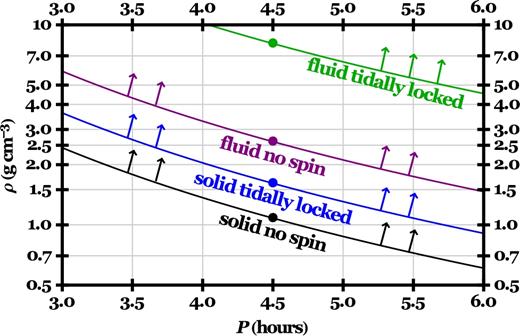
The relation between density (ρ) and orbital period (P) of a strengthless spherical homogeneous rubble pile which resides just at the Roche radius (equation 5); tidally locked rubble piles are in synchronous rotation and arrows indicate stable regions. The relation is general, and is independent of the properties of the central object. Dots indicate the orbital period of the likely disintegrating asteroid at WD 1145+017.
All of the bodies in the figure are strengthless. Incorporating strength would complicate equations (1–4), and the resulting curves would be different. The fluid case is not important for the numerical aspects of our study, but was included in Fig. 1 and Table 1 for comparison with and clarification of existing literature on Roche radii formulations. In contrast to fluids, granular materials, in general, can withstand considerable shear stress when they are under pressure (section 4.2 of Mann, Nakamura & Mukai 2009).
Proportionality constants for different formulations (equations 2–4) of the Roche radius and different generalized strengthless body types. The relations between constants are K = 1.61k, C = 1.63k and |$\mathcal {R} = 0.75K^3$|. The term ‘spinning’ assumes synchronous spinning from being tidally synchronized.
| Body type | K | k | C | |$\mathcal {R}$| | Ref. |
|---|---|---|---|---|---|
| Solid no spin | 1.26 | 0.78 | 1.27 | 1.50 | |
| Solid spinning | 1.44 | 0.89 | 1.45 | 2.24 | a |
| Fluid no spin | 1.69 | 1.05 | 1.70 | 3.62 | b |
| Fluid spinning | 2.46 | 1.53 | 2.49 | 11.2 | c |
| Body type | K | k | C | |$\mathcal {R}$| | Ref. |
|---|---|---|---|---|---|
| Solid no spin | 1.26 | 0.78 | 1.27 | 1.50 | |
| Solid spinning | 1.44 | 0.89 | 1.45 | 2.24 | a |
| Fluid no spin | 1.69 | 1.05 | 1.70 | 3.62 | b |
| Fluid spinning | 2.46 | 1.53 | 2.49 | 11.2 | c |
4 NUMERICAL METHODS
The analysis from the last section shows that knowledge of P can provide strong constraints on ρ. We explore this possibility in the case of WD 1145+017 with numerical simulations of rubble piles, which are aggregates bound together by self-gravity. We used the N-body gravity tree code pkdgrav (Stadel 2001), which has been modified with the ability to detect and resolve collisions amongst individual particles (Leinhardt, Richardson & Quinn 2000; Richardson et al. 2000).
4.1 Common properties
Our simulations required us to specify a central mass and semimajor axis. We chose values which correspond to P ≈ 4.5 h (M⊙ = 0.60 M⊙ and a = 0.0054 au) for all simulations because our focus is on modelling the WD 1145+017 system. We adopted a constant timestep of 50 s for all simulations, a choice which is sufficient to resolve the collisions within each rubble pile (see section 5.3 of Veras et al. 2014a for details).
4.2 Other parameter choices
Other parameters that we varied amongst different simulations include rubble pile structure, number of particles, bulk density ρ and mass M (and hence radius R), plus eccentricity e and spin. See Table A1 for the full list of simulations; three highly referenced simulations are repeated here in Table 2 for demonstration purposes. The table columns are as follows.
Packing type. We created our rubble piles with two different internal packing structures: (1) hexagonal closest packing (HCP; Leinhardt et al. 2000) and (2) random packing. See Fig. 2 for a visual comparison.
Differentiated. This column indicates if the rubble pile was homogeneous or differentiated. The differentiated rubble piles all contained a ‘core’ (green particles in Fig. 2; image B2) and ‘mantle’ (white particles in Fig. 2; image B2). Each type of particle has different properties: each core particle was four times more massive than each mantle particle although all particles had the same size. For these rubble piles, about 35 per cent of particles were core particles.
Number of particles. The vast majority of our simulations contained about 5000 particles, which is a well-justified choice (e.g. Leinhardt et al. 2012; Veras et al. 2014a) because disruption properties have been shown to be independent of particle number until it becomes smaller than roughly 1000. Some long-duration simulations necessarily featured smaller number of particles due to computational limitations.
Density. Our choices for ρ (1.0−4.6 g cm−3) were motivated by Fig. 1 and encompassed the Roche radius regions for solid parent bodies which may be spinning, and a fluid parent body with no spin. This range is reasonable but not exhaustive: the differentiated bodies limit the density on the upper end because the density of the core would be too high if the bulk density was much above 4.6.
Mass. We have considered different parent body masses, even though theoretically tidal disruption of a strengthless body should be scale-independent for any asteroid size (and therefore be independent of mass for a set density; see Solem 1994). We sampled seven orders of magnitude in parent body mass (M = 1016–1022 kg), a range which is bounded from below by parent bodies whose mutual co-orbital interactions would produce period variations on the order of tenths of seconds (Gurri et al. 2017) and from above based on when instability might set in at a significant level (Veras, Marsh & Gänsicke 2016b). Planet-mass objects are not assumed to frequently enter white dwarf Roche radii (Veras et al. 2013a; Mustill et al. 2014; Veras & Gänsicke 2015; Veras et al. 2016a; Veras 2016b) unless they are smaller than the terrestrial planets and, perhaps, are perturbed by a stellar companion (Hamers & Portegies Zwart 2016; Petrovich & Muñoz 2016).
Radius. The radius was simply computed from our choices of M and ρ.
e (eccentricity). Observations so far do not constrain eccentricity, and in the absence of constraints, circular orbits are the simplest assumption. We sampled eccentricities up to 0.2; see Section 5 for more details.
Spin. The values of 0, 1 and 2 indicate no spin, synchronous spin, and twice the synchronous spin rate. A spin value of 0 effectively refers to rotation once per orbit in the direction opposite to the motion in the corotating frame. A spin value of 2 instead refers to rotation once per orbit in the orbit direction in the corotating frame.
Duration. All simulations were run for at least three months (90 d), and some up to 2 yr (730 d). The timespan of 90 d is both computationally feasible and observationally motivated (WD 1145+017 is observed on an almost nightly basis and hence well-sampled over the course of months). This timespan covered nearly 481 orbits. 2 yr corresponds to about 3900 orbits, which represents the overall baseline of observations of the disintegrating asteroid, dating back to the K2 observations reported by Vanderburg et al. (2015).
Outcome. The homogeneous cases result in either full or no disruption (none). The differentiated primary bodies could result in one additional outcome: mantle disruption, where some mantle is lost but the core remains intact.
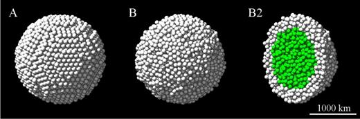
(A) A rubble pile with hexagonal closest packing (HCP) of 5003 particles. (B) A randomly packed differentiated rubble pile consisting of 5000 particles. ( B2) A hemispherical cutaway of B to show the structure (not a distinct initial condition).
| Simulation | Packing | Differe- | Number of | Density | Mass | Radius | e | Spin | Duration | Outcome |
|---|---|---|---|---|---|---|---|---|---|---|
| name | type | ntiated | particles | (g cm−3) | (kg) | (km) | (d) | (disruption type) | ||
| HCP134 | Hexagonal | No | 5003 | 2.60 | 1.0 × 10²² | 1000 | 0.00 | 0 | 90 | full |
| RandDiff19 | Random | Yes | 5000 | 3.50 | 1.2 × 10²² | 1000 | 0.00 | 1 | 90 | mantle |
| RandDiff32 | Random | Yes | 5000 | 3.50 | 1.2 × 10²² | 1000 | 0.01 | 1 | 90 | full |
Overall, computational limitations required us to judiciously choose the resolution with which to sample each parameter range, and how to partition our choices amongst different rubble pile constructions.
5 SIMULATION RESULTS
An observationally relevant question is, can we match the transit observations with a disrupting rubble pile?
5.1 Homogeneous rubble piles
Our first attempt to tackle the answer is to consider the simplest object: a homogeneous one. Also, one of the strictest observational constraints is that the transits are still observed after 2 yr. Therefore, this constraint is the first which we try to replicate. We do so by presenting our results primarily in terms of how quickly the parent body fully disintegrates (Figs 3 and 4). We consider a rubble pile to have disrupted after the mass of the most massive remaining clump is less than one per cent of mass of the original rubble pile. This disruption process for homogeneous rubble piles is illustrated in Fig. 5.
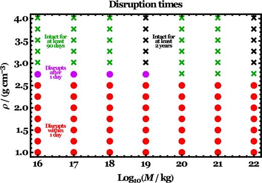
Disruption characteristics for homogeneous HCP progenitors as a function of parent body mass (M) and density (ρ) for circular orbits. Dots illustrate rubble piles which disrupted (HCP1 to HCP53) within one day (red dots) or between one day and one month (purple dots). Crosses represent rubble piles which remained stable throughout their simulations (HCP54 to HCP111), with durations of 90 d (green crosses) or 2 yr (black crosses). The density boundary between disruption and remaining intact is sharp, and is between 2.5 and 3.0 g cm−3 for all masses sampled.
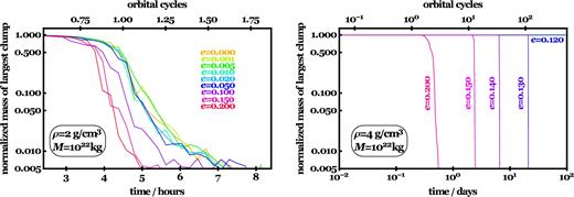
Disruption time-scales for M = 1022 kg, different eccentricities (shown on plots), and two different parent body densities (2 g cm−3, left-hand panel; 4 g cm−3, right-hand panel). Included on the figure are all simulations labelled HCP112 through HCP133 from Table A1 (the horizontal curves for HCP120 to HCP129 in the right-hand panel all overlap). In the left-hand panel, all parent bodies fully disrupt within two orbits, regardless of eccentricity; generally, the higher the eccentricity, the quicker the dissipation. The right-hand panel demonstrates this correlation clearly (a disruption time-scale of three months occurs for some e value between 0.12 and 0.13).
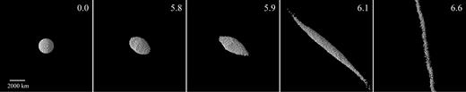
The disruption of a homogeneous hexagonal closest packing (HCP) rubble pile from simulation HCP134 (ρ = 2.6 g cm−3, e = 0). The images are shown in the rotating frame, where left is radially towards the white dwarf and the direction of the orbit is towards the top of the page. The white numbers in the upper part of each panel refer to the number of orbits. An animation accompanying this figure is available online.
5.1.1 Density constraints
Fig. 3 demonstrates disruption times as a function of M and ρ (for simulation details see Table A1) for rubble piles on circular orbits. The dots consist of all rubble piles which disrupted within 90 d; nearly all of these are red dots, indicating disruption within one day. Alternatively, the crosses signify rubble piles which remained intact throughout the duration of the simulation; green crosses represent our standard numerical resolution 90-d simulations and black crosses represent lower numerical resolution 2-yr simulations. The boundary between the dots and crosses, at ρ ≈ 2.5–3.0 g cm−3, is sharp. The plot illustrates the strong sensitivity of disruption to this density boundary, and the relative insensitivity to mass.
5.1.2 Eccentricity constraints
The last section demonstrates that homogeneous primary bodies on circular orbits either disrupt quickly or not at all. These two possibilities do not aid in the interpretation of the observations. Therefore, here we consider non-zero eccentricities. These might allow a rubble pile to dip in-and-out of the Roche radius, shedding some mass during every pericentre passage.
Fig. 4 displays results for simulations of non-circular rubble piles. The simulations in the figure utilize the same semimajor axis as the zero-eccentricity simulations, so that the variations seen are strongly dependent on the decreasing periapse at increasing eccentricity. The plots suggest that for a sufficiently high bulk density (ρ ≳ 2.5 g cm−3 from Fig. 3), there exists a critical eccentricity below which the parent body will remain intact for at least three months. For ρ = 2 g cm−3 (left-hand panel) rubble piles disrupt even on circular orbits, and increasing eccentricity speeds up the disruption (from about 8 h to 5 h). In the right-hand panel, where ρ = 4 g cm−3, this critical eccentricity lay in-between 0.12 and 0.13. Further, the right-hand panel indicates a clearly monotonic trend between increasing eccentricity and disruption time: e = 0.20 corresponds to disruption within a day, whereas rubble piles with 0.14 ≤ e ≤ 0.15 disrupt within a week, and those with e = 0.13 take about a month to break apart.
5.2 Simulation results for differentiated rubble piles
Our results with homogeneous rubble piles could not explain the constant periodic signal or the transient signals over a 2 yr period. Therefore, motivated by Leinhardt et al. (2012), who suggested that a differentiated body might allow for partial disruption, we also adopted a differentiated rubble pile. This assumption is realistic because the primary body could easily be large enough (like the asteroid Vesta; Gurri et al. 2017; Rappaport et al. 2016) to be differentiated. For differentiated bodies, the packing type for rubble piles has a more pronounced effect than in the homogeneous case. Therefore, for greater realism, all of our differentiated rubble piles were randomly packed (consequently, because of the lower packing efficiency, these rubble piles will disrupt more easily; see Figs 2 and 12).
5.2.1 Physics of disruption
The disruption of differentiated rubble piles is more complex than those of homogeneous ones, and has been thoroughly described in Canup (2010) and Leinhardt et al. (2012). We do not repeat their detailed analyses here, but rather just emphasize some of the important points below, and focus instead on the implications for the WD 1145+017 system. Overall, our simulations here are consistent with the behaviour seen in those works.
We characterize the outcome of disrupting a rubble pile with a mantle and core in one of three ways: (i) no disruption, (ii) mantle disruption and (iii) full disruption.
Mantle disruption is shown in Fig. 6 (simulation RandDiff19) and in the accompanying online animation. In this case, the green core particles remain in place and hidden from view as the white mantle particles are slowly stripped off. The streaming occurs at the L1 and L2 Lagrange points after the rubble pile has been distorted into the shape of a lemon. This process reproduces the schematic in fig. A1 of Rappaport et al. (2016), except for the major difference that in our numerical simulations, particles stream off from both L1 and L2, as opposed to just L1. The streaming is not symmetrical from both ends of the parent body, and up to 20 per cent more of the shorn-off particles emanates from one Lagrangian point than the other (see Section 6). The streaming of particles increases the density of the rubble pile, which allows it to subsequently resist disruption. Therefore, after about four orbits, the mantle stripping becomes intermittent. The core density is high enough for the core particles to remain protected from escape.
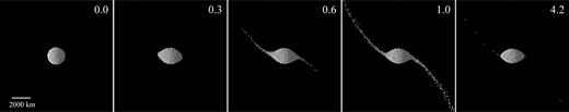
Mantle disruption of a differentiated synchronously spinning rubble pile on a circular orbit with ρ = 3.5 g cm−3 (simulation RandDiff19). The white particles are mantle particles, and the green core particles underneath remain hidden. After about half of an orbit, mantle particles start streaming from the L1 and L2 Lagrange points. After about four orbits, the streaming became intermittent. An animation accompanying this figure is available online.
Full disruption occurs when, subsequent to mantle stripping, the remnant core is not dense enough to resist breakup. This situation is visualized in Fig. 7 (simulation RandDiff32), whose rubble pile is equivalent to that in Fig. 6, except placed on an e = 0.1 orbit. After three orbits, most of the mantle has already separated and is in the process of forming a ring. After four orbits, the entire pile has catastrophically disrupted.
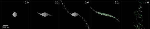
Similar to Fig. 6, except for the case of complete disruption with e = 0.10 (simulation RandDiff32). Subsequent to mantle stripping, the core is not dense enough to resist disruption, and both the white mantle particles and green core particles are visible after three orbits. An animation accompanying this figure is available online.
The trajectory of the stripped off particles forms a ring, just as in the homogeneous case. In Fig. 8, we illustrate this time sequence for the mantle disruption in Fig. 6. After about 10 orbits, the particles have covered an arc halfway around the white dwarf. After about 20 orbits, a full ring has formed, albeit one which contains inhomogeneities. We discuss ring filling times in Section 6.
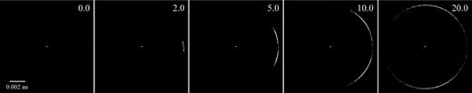
Spreading of stripped particles around the white dwarf (located at the centre) for the mantle disruption in Fig. 6 (simulation RandDiff19). The disrupting rubble pile is at the same position in each panel, centre-right. Rubble pile particles have been inflated to enhance their visibility. An animation accompanying this figure is available online.
Because the particles are stripped off from L1 and L2, they orbit at slightly different distances than does the centre of the rubble pile. Consequently, these particles have slightly different (both larger and shorter) orbital periods than the parent body; see Section 6 for more details.
In order to visualize this difference in orbital period from our simulations, in Fig. 9, we have zoomed-in on the top-left arc of the rightmost panel of Fig. 8. This close-up illustrates both the scale of the annulus, and regions of clumpiness and voids. For M = 1020 kg and 1022 kg parent bodies, the difference in orbital periods from particles on each end of the annulus is on the order of, respectively, a couple tens of seconds, and about 100 s. In this regard, the M = 1020 kg case better matches the orbital period differences given by fig. A3 and equation A11 of Rappaport et al. (2016) and table 1 of Gänsicke et al. (2016). Further, this mass is consistent with the estimates given by Gurri et al. (2017) and Rappaport et al. (2016). The slight excess difference that we see over Rappaport et al.'s (2016) calculation is likely due to collisions in the forming ring.
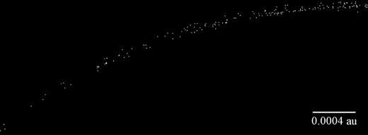
Close-up of the rightmost panel of Fig. 8 (simulation RandDiff19), illustrating annular extent, clumpiness and voids. Particles have been inflated to enhance their visibility.
5.2.2 Transit model
How do these disruption simulations relate to observable photometric transits? WD 1145+017 features some of the most spectacular transit curves of any exoplanetary system, with transit depths reaching 60 per cent, transit features appearing and disappearing on a nightly basis, and some appearing over multiple nights. The periods of the individual transits are stable to a few seconds (table 1 of Gänsicke et al. 2016 and table 4 of Rappaport et al. 2016) even though they differ by up to tens of seconds. In other words, the individual periods are seen to be more stable than their spread among different fragments. Rappaport et al. (2016) suggested that the transit curves in WD 1145+017 may be a result of fragments which break off from a single asteroid. Because we have found that mantle stripping is intermittent, this process could produce fragments which occasionally obscure the light from the white dwarf and create detectable dips in photometric light curves.
Our gravity-only simulations are too simplistic to reproduce the detail in these transit curves, particularly because they arise from dust- and gas-streaming off the fragments rather than from geometrical blocking of the white dwarf by solid bodies. Nevertheless, we have created a transit model from our simulations by inflating the size of our particles which stream away from the disrupted rubble pile. The flux was calculated by dividing the face of the white dwarf into about 27 000 pixels, and counting the number which were not obscured by the transiting fragments.
Fig. 10 displays the result, in two consecutive orbits offset by flux. Here, we have used only the particles which emanated from the rubble pile (which is shown in Fig. 6; simulation RandDiff19) during the previous 50 orbits. The choice of 50 orbits is arbitrary, but represents the idea that fragments are only ‘active’ – i.e. expelling a cloud of gas or dust – for a finite time.1 The time shown is a few hundred orbits after the start of the run, once the rate of fragment escape has slowed. Following Gänsicke et al. (2016), we also introduced two scaling factors: (i) the particle sizes were inflated to four times the size of the white dwarf (in order to achieve appropriate durations) and (ii) the transit depths were scaled such that the maximum depth was 0.5. The line-of-sight inclination was assumed to be offset by 2|$_{.}^{\circ}$|25 from an edge-on orientation, following the assumption in Gänsicke et al. (2016).
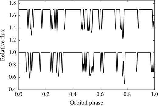
Illustrative model of photometric transit depths due to mantle stripping, a process which intermittently streams particles off of a rubble pile. Shown here are two consecutive orbits offset in flux. The rubble pile used here was from simulation RandDiff19 (Fig. 6), with particles suitably inflated. See the main text for more details.
The primary benefit of this simulation is to show that (i) the transit durations over a single orbit are commensurate with those actually observed, and (ii) the non-uniformity of the transit features may be reproduced by mantle stripping. Because the stripping is intermittent, this process may help explain the transience of some of the observed features.
5.2.3 Density constraints
Our simulations suggest that the process of mantle disruption might play an important role in the dynamics of WD 1145+017. A natural accompanying question is, for what values of ρ does mantle disruption occur? In order to pursue an answer, and informed by the bounds imposed from our homogenous rubble pile results, we have simulated differentiated rubble piles with 11 different bulk core plus mantle densities from 2.5 to 4.0 g cm−3.
We present the results in Fig. 11, which has a similar format to Fig. 4 and contains the simulations labelled RandDiff1 to RandDiff22 in Table A1. Here, however, mantle disruption is indicated by a slight decrease, at the few to tens of per cent level, in normalized mass of the largest remaining clump, before levelling off. Note that mantle or full disruption occurs in every simulation in the figure. The amount of material lost decreases for higher densities; at the high end (ρ = 4.0 g cm−3), in the left- and right-hand panels, respectively, 2.1 and 3.9 per cent of the total mass was lost. For ρ < 3.2 g cm−3, mantle disruption can be observed to occur for a few hours before full disruption occurs more quickly.
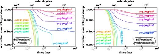
Disruption time-scales for differentiated rubble piles, where the core particle mass is quadruple that of the mantle particle mass (simulations RandDiff1 to RandDiff22). The rubble piles are on circular orbits and have either no spin (left-hand panel) or synchronous spin, equivalent to being tidally locked (right-hand panel). The slight decrease in mass at the tens of percent level seen in the curves with ρ ≥ 3.2 g cm−3 indicate mantle disruption. Full disruption occurs for ρ ≤ 3.1 g cm−3. This robust constraint on density, although specific to the rubble pile modelled, is similar to the robustness of the density constraints observed in Figs 3 and 4.
Comparison of the two panels in the figure indicates that the initial spin of the rubble pile makes little difference to the outcomes, except at the boundaries of the disruption regimes. For the particular differentiated rubble piles we sampled in this work (with a core four times more massive than the mantle), the transition density between mantle disruption and full disruption occurs at ρ = 3.1 g cm−3. At this density, a synchronously spinning rubble pile disrupts an order of magnitude more quickly than a rubble pile with no initial spin.
Although the boundary defined by ρ = 3.1 g cm−3 is strongly linked to the structure of the differentiated rubble pile which we adopted, the clear division between disruption regimes on the figure suggests that other rubble pile constructions will yield similarly robust constraints.
5.2.4 General constraints
Other shape geometries may need to be considered when modelling disruption of parent bodies in other systems. In fact, the results of our simulations might aid in future efforts, a prospect which we consider in this subsection.
Unlike for homogeneous rubble piles, which either disrupt fully or not at all, differentiated rubble piles could undergo no disruption, mantle disruption or full disruption. In order to better quantify the parameter regimes encompassing these ternary outcomes, we present Figs 12 and 13.
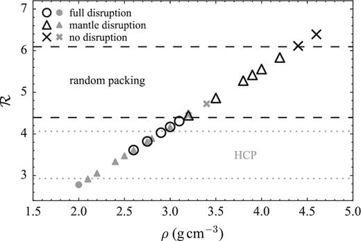
Boundaries between the regimes of ‘full disruption’, ‘mantle disruption’ and ‘no disruption’. The darker hollow symbols refer to simulations with randomly packed rubble piles, and the lighter filled symbols to outcomes with hexagonal-closely packed (HCP) rubble piles. The boundaries are approximated by the dashed lines, and are in good agreement with fig. 2 of Leinhardt et al. (2012).
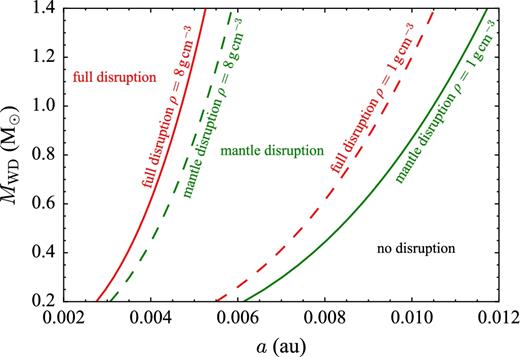
Pinpointing the three regimes where full disruption, mantle disruption and no disruption occur as a function of stellar mass (MWD) and parent body semimajor axis (a). The regions are identified by the horizontal labels. The curves are based on the dashed lines in Fig. 12 and are applicable only for our randomly packed rubble pile simulations.
Fig. 12 links disruption with |$\mathcal {R}$| and ρ through equations (4) and (5). The darker symbols represent simulations RandDiff2 through RandDiff11, plus RandDiff23, RandDiff24 and RandDiff25. The lighter symbols represent the outcomes for additional simulations (HCPDiff1 to HCPDiff11). The arbitrarily drawn dashed lines then approximate the critical values (4.4 and 6.1) of |$\mathcal {R}$| which separate the three regimes.
Fig. 12 can be compared directly to the bottom plot of fig. 2 of Leinhardt et al. (2012), which presents outcomes of tidal disruption simulations of randomly packed differentiated moons. Although they sampled a range of a, and hence P, the agreement with the critical values of 4.4 and 6.1 is good, to within one unit of |$\mathcal {R}$| in each case. Any differences could be attributed to the details of the packing geometry, including the bulk radius.
These critical values of 4.4 and 6.1 were then used to create Fig. 13, which ignores our knowledge of P. This figure approximates the boundaries between the disruption regimes (red = full disruption, green = mantle disruption, black = no disruption) in (a, MWD) space, for all possible white dwarf masses, where two extreme densities (1 g cm−3 and 8 g cm−3) are given. The solid lines provide absolute bounds. In the region to the left of the red solid line, full disruption always occurs. In the region to the right of the green solid line, no disruption ever occurs. In between those two lines, any three possibilities may occur depending on the choice of ρ. If the asteroid is less differentiated or centrally concentrated, then these curves would all shift rightwards.
Both figures represent useful tools for quick identification of a disruption regime for future discoveries of disintegrating bodies around stars. These stars need not be restricted to white dwarfs. In fact, several bodies disintegrating around main-sequence stars are now known (Rappaport et al. 2012, 2014; Croll et al. 2014; Bochinski et al. 2015; Sanchis-Ojeda et al. 2015).
6 DISCUSSION
6.1 Roche radius location
We can now return to the question of whether the disrupting asteroid is within the Roche radius of WD 1145+017. Consider that (1) the observational data suggest that the asteroid has not undergone full disruption for over 2 yr, (2) we have shown that an asteroid which remains intact for this long has ρ ≳ 3.1 g cm−3 on a near-circular orbit, (3) the density which corresponds to the Roche radius for this white dwarf is, for a solid, tidally locked body, 1.6 g cm−3, (4) we have shown that mantle disruption can qualitatively reproduce the intermittent transit features which are observed.
These statements imply that the parent body is not within the Roche radius for its bulk density, but rather just outside, and undergoing mantle disruption. Some caveats which might negate this conclusion are if the asteroid's shape is significantly non-spherical, the asteroid is differentiated in a complex manner, or if the asteroid's mass contains a significant amount of non-solid matter. These cases all represent viable, interesting and important topics for future studies. Objects like 67P/Churyumov–Gerasimenko hint at the complexity of small Solar system bodies, and similar bodies could maintain an internal reservoir of volatiles even throughout the giant branch phases of stellar evolution (Jura & Xu 2010; Jura et al. 2012; Malamud & Perets 2016).
The details of the disruption which we have shown here are different than those envisaged by Rappaport et al. (2016). Here, we see mass streaming from both L1 and L2 points. Further, we find that the relative fraction of particles escaping from L1 is slightly greater than those from L2, with the disparity increasing for higher bulk densities. In particular, for ρ = 3.9 g cm−3, 56 per cent come from L1, whereas for both ρ = 4.0 g cm−3 and ρ = 4.2 g cm−3, 59 per cent originate from L1. These differences are observationally constrained, although only material with shorter orbits is visible (Gänsicke et al. 2016; Rappaport et al. 2016). Perhaps the fragments with longer periods are not currently active, or that the imbalance between streaming from L1 and L2 becomes larger with time. K2 data did show some very weak signals at longer periods, but their reality could not be confirmed independently, as those signals are below the sensitivity threshold for ground-based observations.
If the asteroid indeed lies just outside of the Roche radius, then how did it arrive at a nearly circular orbit at that location? One possibility is that sustained gas ejection may be strong enough to appreciably decay the orbit of close minor planets (e.g. equations 32– 33 of Perez-Becker & Chiang 2013), although the exact manner of the orbital evolution may be nontrivial (Boué et al. 2012; Veras et al. 2013b; Dosopoulou & Kalogera 2016a,b). An alternative (A. Johansen, private communication) is that the asteroid represents a second-generation minor planet which grew out of smaller debris from a disrupted planetesimal which accumulated outside of the Roche radius, an idea previously proposed for Solar system moons (e.g. Crida & Charnoz 2012). Charnoz et al. (2011) suggested that the inner mid-sized moons of Saturn (Mimas, Enceladus, Tethys, Dione and Rhea) could all have been formed by a viscously spreading massive ring which was itself the result of a large disruptive impact. Phobos and Deimos (Mars's moons) could have formed close enough to their parent planet that they have since spiraled in close to Mars due to tidal decay of the orbit (Rosenblatt & Charnoz 2012).
6.2 Ring filling time
We have shown that disrupting rubble piles form rings. How efficiently does the debris spread around the white dwarf? We approach this question both analytically and with the numerical output. A key caveat to both approaches is that gas drag is neglected, which may play a significant role in the WD 1145+107 system.2 Also, the analytical approach ignores collisions, which are treated in the pkdgrav simulations.
6.2.1 Analytic filling times
6.2.2 Numerical filling times
Numerically, one way to determine how quickly particles spread into a ring is to consider the time evolution of the centre of mass of the particles, rCOM. Initially, rCOM ≈ a ≈ 92RWD, assuming RWD = 8750 km (a fiducial white dwarf radius; Veras et al. 2014a). As the rubble pile disrupts and the particles spread into a ring, this centre of mass will gradually move towards the centre of the white dwarf. Consequently, a uniform ring is formed as rCOM → 0. However, as rCOM approaches zero, it oscillates as ring particles overtake each other, and potentially collide. This movement ceases to be monotonic, and inhomogeneities in the ring will show up as non-zero values of rCOM.
6.2.3 Results
In Fig. 14, we plot the time evolution of rCOM for all homogeneous HCP rubble piles that are disrupted. Overplotted as stars, triangles and a square are the analytical estimates of the filling time from equation (10). Quantifying the extent of the agreement between the analytics and numerics is not possible unless one defines the meaning of a ring which has been ‘filled’: the curves in Fig. 14 appear to ‘bounce’ on the x-axis several times before settling. Equation (10) best reproduces a point in-between the second and third bounce.
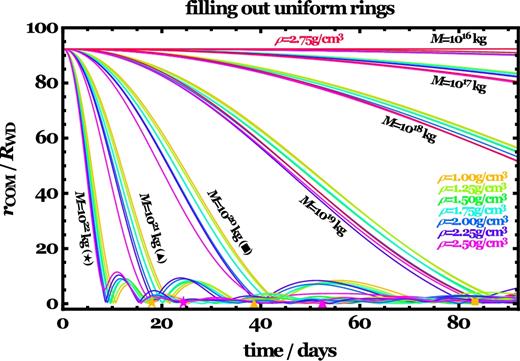
Ring filling times. Plotted is the time evolution of rCOM, which is the distance between the centre of mass of the rubble pile particles and the centre of the white dwarf. As the rubble pile disrupts and a ring fills out, this distance decreases. When rCOM = 0, a uniform ring has been created. Inhomogeneities (clumpiness and voids) in the ring result in the ‘bounces’ along the x-axis. Plotted symbols (stars for M = 1022 kg, triangles for M = 1021 kg, squares for M = 1020 kg; yellow for ρ = 1.0 g cm−3 and pink for ρ = 2.5 g cm−3) indicate the analytical predictions for the filling times of asteroids which are assumed to instantaneously disrupt at their orbital pericentres (equations 8 and 10).
Some trends from the figure are worth noting, particularly because of their potential use for interpreting future observations: (i) the circularization time decreases with increasing mass, (ii) the ‘bounciness’ increases with increasing mass, (iii) rubble piles with M ≳ 1020 kg generally spread out into full rings within about three months and (iv) for a given mass, higher density rubble piles more quickly achieve particle coverage throughout the orbit, but do not necessarily evenly fill out the ring more quickly or smoothly.
The figure demonstrates that the ring filling times range from 10 to 100 d for 1019 kg ≲ M ≲ 1022 kg. Although this time-scale fits within the baseline of observations, the ring is not directly observed. One possible reason is that the ring is collisionally eroded; another is that the newly disrupted pieces of mantle are not active. However, theoretical models which include dust and/or gas might better link observed infrared excess (indicating dust) or circumstellar gas (Xu et al. 2016) with ring formation.
7 CONCLUSION
The properties of the asteroid disintegrating around white dwarf WD 1145+017 are poorly constrained observationally. Theoretical work, however, can help remedy this shortfall, and in this case suggests that the disintegrating asteroid orbiting WD 1145+017 appears to reside just outside of the bulk density Roche radius.
In particular, we have modelled the tidal disruption of strengthless rubble piles with an orbital period equal to that of the longest-lasting observed transit signature. We found robust constraints on density (Figs 3 and 11) and eccentricity (Fig. 4), and weak constraints on mass (Fig. 3) and spin (Fig. 11) (but see the last paragraph of Section 5.2.1). By modelling both homogeneous and differentiated rubble piles, we found that ρ ≲ 2.75 g cm−3 ensures disruption within one day, whereas ρ ≳ 3.10 g cm−3 guarantees that rubble piles on circular orbits will remain intact for at least 2 yr. Nevertheless, the intact differentiated rubble piles all undergo mantle disruption, which produces intermittent streams of particles which may contribute to the observed photometric transit dips (Fig. 10). If the eccentricity of the disrupting object exceeds 0.130, then it is unlikely to remain intact for more than one month unless ρ > 4.0 g cm−3.
Useful ancillary results include figures which may be applicable for studies of disruption around other stars. These figures include a mass-free relation between orbital period and density (Fig. 1, and equation 5) and parameter-space locations where we can expect to find mantle disruption versus full disruption (Figs 12 and 13).
We must caution that our seemingly robust results for WD 1145+017 rely on several assumptions: (i) the parent body is spherical, (ii) the parent body is strengthless and (iii) the parent body or its fragments are not affected by the extant dust or gas in the system. Relaxing these assumptions (e.g. Metzger, Rafikov & Bochkarev 2012; Movshovitz, Asphaug & Korycansky 2012; Schwartz, Richardson & Michel 2012) as new observations warrant might place stricter physical constraints on the system.
Acknowledgments
We thank the referee for a careful read-through of the manuscript, and valuable comments. DV and BTG have received funding from the European Research Council under the European Union's Seventh Framework Programme (FP/2007-2013)/ERC Grant Agreement no. 320964 (WDTracer). PJC and ZML acknowledge support from the Natural Environment Research Council (grant number: NE/K004778/1).
If we had not implemented a cutoff, then the simulation would have been saturated as fragments were spread into a ring, but not removed.
Gas is likely produced from sublimation and/or collisions of solid particles. The most recent substantial attempt to model this interaction between gas and dust (Metzger et al. 2012) indicates a complexity which is beyond the scope of this work.
REFERENCES
SUPPORTING INFORMATION
Supplementary data are available at MNRAS online.
LastMovies.tgz
Please note: Oxford University Press is not responsible for the content or functionality of any supporting materials supplied by the authors. Any queries (other than missing material) should be directed to the corresponding author for the article.
APPENDIX A: SIMULATION TABLE
Summary of simulations. The radii are rounded to two significant digits. Bold entries indicate important variables which were varied within each set.
| Simulation | Packing | Differe- | Number of | Density | Mass | Radius | e | Spin | Duration | Outcome |
|---|---|---|---|---|---|---|---|---|---|---|
| name | type | -ntiated | particles | (g cm−3) | (kg) | (km) | (d) | (disruption type) | ||
| HCP1 | Hexagonal | No | 5003 | 1.00 | 1016 | 14 | 0.00 | 0 | 90 | Full |
| HCP2 | Hexagonal | No | 5003 | 1.00 | 1017 | 29 | 0.00 | 0 | 90 | Full |
| HCP3 | Hexagonal | No | 5003 | 1.00 | 1018 | 62 | 0.00 | 0 | 90 | Full |
| HCP4 | Hexagonal | No | 5003 | 1.00 | 1019 | 130 | 0.00 | 0 | 90 | Full |
| HCP5 | Hexagonal | No | 5003 | 1.00 | 1020 | 290 | 0.00 | 0 | 90 | Full |
| HCP6 | Hexagonal | No | 5003 | 1.00 | 1021 | 620 | 0.00 | 0 | 90 | Full |
| HCP7 | Hexagonal | No | 5003 | 1.00 | 1022 | 1300 | 0.00 | 0 | 90 | Full |
| HCP8 | Hexagonal | No | 5003 | 1.25 | 1016 | 12 | 0.00 | 0 | 90 | Full |
| HCP9 | Hexagonal | No | 5003 | 1.25 | 1017 | 27 | 0.00 | 0 | 90 | Full |
| HCP10 | Hexagonal | No | 5003 | 1.25 | 1018 | 58 | 0.00 | 0 | 90 | Full |
| HCP11 | Hexagonal | No | 5003 | 1.25 | 1019 | 120 | 0.00 | 0 | 90 | Full |
| HCP12 | Hexagonal | No | 5003 | 1.25 | 1020 | 270 | 0.00 | 0 | 90 | Full |
| HCP13 | Hexagonal | No | 5003 | 1.25 | 1021 | 580 | 0.00 | 0 | 90 | Full |
| HCP14 | Hexagonal | No | 5003 | 1.25 | 1022 | 1200 | 0.00 | 0 | 90 | Full |
| HCP15 | Hexagonal | No | 5003 | 1.50 | 1016 | 12 | 0.00 | 0 | 90 | Full |
| HCP16 | Hexagonal | No | 5003 | 1.50 | 1017 | 25 | 0.00 | 0 | 90 | Full |
| HCP17 | Hexagonal | No | 5003 | 1.50 | 1018 | 54 | 0.00 | 0 | 90 | Full |
| HCP18 | Hexagonal | No | 5003 | 1.50 | 1019 | 120 | 0.00 | 0 | 90 | Full |
| HCP19 | Hexagonal | No | 5003 | 1.50 | 1020 | 250 | 0.00 | 0 | 90 | Full |
| HCP20 | Hexagonal | No | 5003 | 1.50 | 1021 | 540 | 0.00 | 0 | 90 | Full |
| HCP21 | Hexagonal | No | 5003 | 1.50 | 1022 | 1200 | 0.00 | 0 | 90 | Full |
| HCP22 | Hexagonal | No | 5003 | 1.75 | 1016 | 11 | 0.00 | 0 | 90 | Full |
| HCP23 | Hexagonal | No | 5003 | 1.75 | 1017 | 24 | 0.00 | 0 | 90 | Full |
| HCP24 | Hexagonal | No | 5003 | 1.75 | 1018 | 51 | 0.00 | 0 | 90 | Full |
| HCP25 | Hexagonal | No | 5003 | 1.75 | 1019 | 110 | 0.00 | 0 | 90 | Full |
| HCP26 | Hexagonal | No | 5003 | 1.75 | 1020 | 240 | 0.00 | 0 | 90 | Full |
| HCP27 | Hexagonal | No | 5003 | 1.75 | 1021 | 510 | 0.00 | 0 | 90 | Full |
| HCP28 | Hexagonal | No | 5003 | 1.75 | 1022 | 1100 | 0.00 | 0 | 90 | Full |
| HCP29 | Hexagonal | No | 5003 | 2.00 | 1016 | 11 | 0.00 | 0 | 90 | Full |
| HCP30 | Hexagonal | No | 5003 | 2.00 | 1017 | 23 | 0.00 | 0 | 90 | Full |
| HCP31 | Hexagonal | No | 5003 | 2.00 | 1018 | 49 | 0.00 | 0 | 90 | Full |
| HCP32 | Hexagonal | No | 5003 | 2.00 | 1019 | 110 | 0.00 | 0 | 90 | Full |
| HCP33 | Hexagonal | No | 5003 | 2.00 | 1020 | 230 | 0.00 | 0 | 90 | Full |
| HCP34 | Hexagonal | No | 5003 | 2.00 | 1021 | 490 | 0.00 | 0 | 90 | Full |
| HCP35 | Hexagonal | No | 5003 | 2.00 | 1022 | 1100 | 0.00 | 0 | 90 | Full |
| HCP36 | Hexagonal | No | 5003 | 2.25 | 1016 | 10 | 0.00 | 0 | 90 | Full |
| HCP37 | Hexagonal | No | 5003 | 2.25 | 1017 | 22 | 0.00 | 0 | 90 | Full |
| HCP38 | Hexagonal | No | 5003 | 2.25 | 1018 | 47 | 0.00 | 0 | 90 | Full |
| HCP39 | Hexagonal | No | 5003 | 2.25 | 1019 | 102 | 0.00 | 0 | 90 | Full |
| HCP40 | Hexagonal | No | 5003 | 2.25 | 1020 | 220 | 0.00 | 0 | 90 | Full |
| HCP41 | Hexagonal | No | 5003 | 2.25 | 1021 | 470 | 0.00 | 0 | 90 | Full |
| HCP42 | Hexagonal | No | 5003 | 2.25 | 1022 | 1000 | 0.00 | 0 | 90 | Full |
| HCP43 | Hexagonal | No | 5003 | 2.50 | 1016 | 9.9 | 0.00 | 0 | 90 | Full |
| HCP44 | Hexagonal | No | 5003 | 2.50 | 1017 | 21 | 0.00 | 0 | 90 | Full |
| HCP45 | Hexagonal | No | 5003 | 2.50 | 1018 | 46 | 0.00 | 0 | 90 | Full |
| HCP46 | Hexagonal | No | 5003 | 2.50 | 1019 | 98 | 0.00 | 0 | 90 | Full |
| HCP47 | Hexagonal | No | 5003 | 2.50 | 1020 | 210 | 0.00 | 0 | 90 | Full |
| HCP48 | Hexagonal | No | 5003 | 2.50 | 1021 | 460 | 0.00 | 0 | 90 | Full |
| HCP49 | Hexagonal | No | 5003 | 2.50 | 1022 | 990 | 0.00 | 0 | 90 | Full |
| HCP50 | Hexagonal | No | 5003 | 2.75 | 1016 | 9.5 | 0.00 | 0 | 90 | Full |
| HCP51 | Hexagonal | No | 5003 | 2.75 | 1017 | 21 | 0.00 | 0 | 90 | Full |
| HCP52 | Hexagonal | No | 5003 | 2.75 | 1018 | 44 | 0.00 | 0 | 90 | Full |
| HCP53 | Hexagonal | No | 5003 | 2.75 | 1019 | 95 | 0.00 | 0 | 90 | Full |
| HCP54 | Hexagonal | No | 5003 | 2.75 | 1020 | 210 | 0.00 | 0 | 90 | None |
| HCP55 | Hexagonal | No | 5003 | 2.75 | 1021 | 440 | 0.00 | 0 | 90 | None |
| HCP56 | Hexagonal | No | 5003 | 2.75 | 1022 | 950 | 0.00 | 0 | 90 | None |
| HCP57 | Hexagonal | No | 5003 | 3.00 | 1016 | 9.3 | 0.00 | 0 | 90 | None |
| HCP58 | Hexagonal | No | 5003 | 3.00 | 1017 | 20 | 0.00 | 0 | 90 | None |
| HCP59 | Hexagonal | No | 5003 | 3.00 | 1018 | 43 | 0.00 | 0 | 90 | None |
| HCP60 | Hexagonal | No | 5003 | 3.00 | 1019 | 93 | 0.00 | 0 | 180 | None |
| HCP61 | Hexagonal | No | 3985 | 3.00 | 1019 | 93 | 0.00 | 0 | 365 | None |
| HCP62 | Hexagonal | No | 3011 | 3.00 | 1019 | 93 | 0.00 | 0 | 730 | None |
| HCP63 | Hexagonal | No | 5003 | 3.00 | 1020 | 200 | 0.00 | 0 | 90 | None |
| HCP64 | Hexagonal | No | 5003 | 3.00 | 1021 | 430 | 0.00 | 0 | 90 | None |
| HCP65 | Hexagonal | No | 5003 | 3.00 | 1022 | 930 | 0.00 | 0 | 180 | None |
| HCP66 | Hexagonal | No | 3985 | 3.00 | 1022 | 930 | 0.00 | 0 | 365 | None |
| HCP67 | Hexagonal | No | 3011 | 3.00 | 1022 | 930 | 0.00 | 0 | 730 | None |
| HCP68 | Hexagonal | No | 5003 | 3.25 | 1016 | 9.0 | 0.00 | 0 | 90 | None |
| HCP69 | Hexagonal | No | 5003 | 3.25 | 1017 | 19 | 0.00 | 0 | 90 | None |
| HCP70 | Hexagonal | No | 5003 | 3.25 | 1018 | 42 | 0.00 | 0 | 90 | None |
| HCP71 | Hexagonal | No | 5003 | 3.25 | 1019 | 90 | 0.00 | 0 | 180 | None |
| HCP72 | Hexagonal | No | 3985 | 3.25 | 1019 | 90 | 0.00 | 0 | 365 | None |
| HCP73 | Hexagonal | No | 3011 | 3.25 | 1019 | 90 | 0.00 | 0 | 730 | None |
| HCP74 | Hexagonal | No | 5003 | 3.25 | 1020 | 190 | 0.00 | 0 | 90 | None |
| HCP75 | Hexagonal | No | 5003 | 3.25 | 1021 | 420 | 0.00 | 0 | 90 | None |
| HCP76 | Hexagonal | No | 5003 | 3.25 | 1022 | 900 | 0.00 | 0 | 180 | None |
| HCP77 | Hexagonal | No | 3985 | 3.25 | 1022 | 900 | 0.00 | 0 | 365 | None |
| HCP78 | Hexagonal | No | 3011 | 3.25 | 1022 | 900 | 0.00 | 0 | 730 | None |
| HCP79 | Hexagonal | No | 5003 | 3.50 | 1016 | 8.8 | 0.00 | 0 | 90 | None |
| HCP80 | Hexagonal | No | 5003 | 3.50 | 1017 | 19 | 0.00 | 0 | 90 | None |
| HCP81 | Hexagonal | No | 5003 | 3.50 | 1018 | 41 | 0.00 | 0 | 90 | None |
| HCP82 | Hexagonal | No | 5003 | 3.50 | 1019 | 88 | 0.00 | 0 | 180 | None |
| HCP83 | Hexagonal | No | 3985 | 3.50 | 1019 | 88 | 0.00 | 0 | 365 | None |
| HCP84 | Hexagonal | No | 3011 | 3.50 | 1019 | 88 | 0.00 | 0 | 730 | None |
| HCP85 | Hexagonal | No | 5003 | 3.50 | 1020 | 190 | 0.00 | 0 | 90 | None |
| HCP86 | Hexagonal | No | 5003 | 3.50 | 1021 | 410 | 0.00 | 0 | 90 | None |
| HCP87 | Hexagonal | No | 5003 | 3.50 | 1022 | 880 | 0.00 | 0 | 180 | None |
| HCP88 | Hexagonal | No | 3985 | 3.50 | 1022 | 880 | 0.00 | 0 | 365 | None |
| HCP89 | Hexagonal | No | 3011 | 3.50 | 1022 | 880 | 0.00 | 0 | 730 | None |
| HCP90 | Hexagonal | No | 5003 | 3.75 | 1016 | 8.6 | 0.00 | 0 | 90 | None |
| HCP91 | Hexagonal | No | 5003 | 3.75 | 1017 | 19 | 0.00 | 0 | 90 | None |
| HCP92 | Hexagonal | No | 5003 | 3.75 | 1018 | 40 | 0.00 | 0 | 90 | None |
| HCP93 | Hexagonal | No | 5003 | 3.75 | 1019 | 86 | 0.00 | 0 | 180 | None |
| HCP94 | Hexagonal | No | 3985 | 3.75 | 1019 | 86 | 0.00 | 0 | 365 | None |
| HCP95 | Hexagonal | No | 3011 | 3.75 | 1019 | 86 | 0.00 | 0 | 730 | None |
| HCP96 | Hexagonal | No | 5003 | 3.75 | 1020 | 190 | 0.00 | 0 | 90 | None |
| HCP97 | Hexagonal | No | 5003 | 3.75 | 1021 | 400 | 0.00 | 0 | 90 | None |
| HCP98 | Hexagonal | No | 5003 | 3.75 | 1022 | 860 | 0.00 | 0 | 180 | None |
| HCP99 | Hexagonal | No | 3985 | 3.75 | 1022 | 860 | 0.00 | 0 | 365 | None |
| HCP100 | Hexagonal | No | 3011 | 3.75 | 1022 | 860 | 0.00 | 0 | 730 | None |
| HCP101 | Hexagonal | No | 5003 | 4.00 | 1016 | 8.4 | 0.00 | 0 | 90 | None |
| HCP102 | Hexagonal | No | 5003 | 4.00 | 1017 | 18 | 0.00 | 0 | 90 | None |
| HCP103 | Hexagonal | No | 5003 | 4.00 | 1018 | 39 | 0.00 | 0 | 90 | None |
| HCP104 | Hexagonal | No | 5003 | 4.00 | 1019 | 84 | 0.00 | 0 | 180 | None |
| HCP105 | Hexagonal | No | 3985 | 4.00 | 1019 | 84 | 0.00 | 0 | 365 | None |
| HCP106 | Hexagonal | No | 3011 | 4.00 | 1019 | 84 | 0.00 | 0 | 730 | None |
| HCP107 | Hexagonal | No | 5003 | 4.00 | 1020 | 180 | 0.00 | 0 | 90 | None |
| HCP108 | Hexagonal | No | 5003 | 4.00 | 1021 | 390 | 0.00 | 0 | 90 | None |
| HCP109 | Hexagonal | No | 5003 | 4.00 | 1022 | 840 | 0.00 | 0 | 180 | None |
| HCP110 | Hexagonal | No | 3985 | 4.00 | 1022 | 840 | 0.00 | 0 | 365 | None |
| HCP111 | Hexagonal | No | 3011 | 4.00 | 1022 | 840 | 0.00 | 0 | 730 | None |
| HCP112 | Hexagonal | No | 5003 | 2.00 | 1022 | 1100 | 0.001 | 0 | 90 | Full |
| HCP113 | Hexagonal | No | 5003 | 2.00 | 1022 | 1100 | 0.005 | 0 | 90 | Full |
| HCP114 | Hexagonal | No | 5003 | 2.00 | 1022 | 1100 | 0.010 | 0 | 90 | Full |
| HCP115 | Hexagonal | No | 5003 | 2.00 | 1022 | 1100 | 0.020 | 0 | 90 | Full |
| HCP116 | Hexagonal | No | 5003 | 2.00 | 1022 | 1100 | 0.050 | 0 | 90 | Full |
| HCP117 | Hexagonal | No | 5003 | 2.00 | 1022 | 1100 | 0.100 | 0 | 90 | Full |
| HCP118 | Hexagonal | No | 5003 | 2.00 | 1022 | 1100 | 0.150 | 0 | 90 | Full |
| HCP119 | Hexagonal | No | 5003 | 2.00 | 1022 | 1100 | 0.200 | 0 | 90 | Full |
| HCP120 | Hexagonal | No | 5003 | 4.00 | 1022 | 840 | 0.001 | 0 | 90 | None |
| HCP121 | Hexagonal | No | 5003 | 4.00 | 1022 | 840 | 0.005 | 0 | 90 | None |
| HCP122 | Hexagonal | No | 5003 | 4.00 | 1022 | 840 | 0.010 | 0 | 90 | None |
| HCP123 | Hexagonal | No | 5003 | 4.00 | 1022 | 840 | 0.020 | 0 | 90 | None |
| HCP124 | Hexagonal | No | 5003 | 4.00 | 1022 | 840 | 0.050 | 0 | 90 | None |
| HCP125 | Hexagonal | No | 5003 | 4.00 | 1022 | 840 | 0.080 | 0 | 90 | None |
| HCP126 | Hexagonal | No | 5003 | 4.00 | 1022 | 840 | 0.090 | 0 | 90 | None |
| HCP127 | Hexagonal | No | 5003 | 4.00 | 1022 | 840 | 0.100 | 0 | 90 | None |
| HCP128 | Hexagonal | No | 5003 | 4.00 | 1022 | 840 | 0.110 | 0 | 90 | None |
| HCP129 | Hexagonal | No | 5003 | 4.00 | 1022 | 840 | 0.120 | 0 | 90 | None |
| HCP130 | Hexagonal | No | 5003 | 4.00 | 1022 | 840 | 0.130 | 0 | 90 | Full |
| HCP131 | Hexagonal | No | 5003 | 4.00 | 1022 | 840 | 0.140 | 0 | 90 | Full |
| HCP132 | Hexagonal | No | 5003 | 4.00 | 1022 | 840 | 0.150 | 0 | 90 | Full |
| HCP133 | Hexagonal | No | 5003 | 4.00 | 1022 | 840 | 0.200 | 0 | 90 | Full |
| HCP134 | Hexagonal | No | 5003 | 2.60 | 1022 | 1000 | 0.00 | 0 | 90 | Full |
| RandDiff1 | Random | Yes | 5000 | 2.50 | 8.9 × 10²¹ | 1000 | 0.00 | 0 | 90 | Full |
| RandDiff2 | Random | Yes | 5000 | 2.60 | 9.3 × 10²¹ | 1000 | 0.00 | 0 | 90 | Full |
| RandDiff3 | Random | Yes | 5000 | 2.75 | 9.8 × 10²¹ | 1000 | 0.00 | 0 | 90 | Full |
| RandDiff4 | Random | Yes | 5000 | 2.90 | 1.0 × 10²² | 1000 | 0.00 | 0 | 90 | Full |
| RandDiff5 | Random | Yes | 5000 | 3.00 | 1.1 × 10²² | 1000 | 0.00 | 0 | 90 | Full |
| RandDiff6 | Random | Yes | 5000 | 3.10 | 1.1 × 10²² | 1000 | 0.00 | 0 | 90 | Full |
| RandDiff7 | Random | Yes | 5000 | 3.20 | 1.1 × 10²² | 1000 | 0.00 | 0 | 90 | Mantle |
| RandDiff8 | Random | Yes | 5000 | 3.50 | 1.2 × 10²² | 1000 | 0.00 | 0 | 90 | Mantle |
| RandDiff9 | Random | Yes | 5000 | 3.80 | 1.4 × 10²² | 1000 | 0.00 | 0 | 90 | Mantle |
| RandDiff10 | Random | Yes | 5000 | 3.90 | 1.4 × 10²² | 1000 | 0.00 | 0 | 90 | Mantle |
| RandDiff11 | Random | Yes | 5000 | 4.00 | 1.4 × 10²² | 1000 | 0.00 | 0 | 90 | Mantle |
| RandDiff12 | Random | Yes | 5000 | 2.50 | 8.9 × 10²¹ | 1000 | 0.00 | 1 | 90 | Full |
| RandDiff13 | Random | Yes | 5000 | 2.60 | 9.3 × 10²¹ | 1000 | 0.00 | 1 | 90 | Full |
| RandDiff14 | Random | Yes | 5000 | 2.75 | 9.8 × 10²¹ | 1000 | 0.00 | 1 | 90 | Full |
| RandDiff15 | Random | Yes | 5000 | 2.90 | 1.0 × 10²² | 1000 | 0.00 | 1 | 90 | Full |
| RandDiff16 | Random | Yes | 5000 | 3.00 | 1.1 × 10²² | 1000 | 0.00 | 1 | 90 | Full |
| RandDiff17 | Random | Yes | 5000 | 3.10 | 1.1 × 10²² | 1000 | 0.00 | 1 | 90 | Full |
| RandDiff18 | Random | Yes | 5000 | 3.20 | 1.1 × 10²² | 1000 | 0.00 | 1 | 90 | Mantle |
| RandDiff19 | Random | Yes | 5000 | 3.50 | 1.2 × 10²² | 1000 | 0.00 | 1 | 90 | Mantle |
| RandDiff20 | Random | Yes | 5000 | 3.80 | 1.4 × 10²² | 1000 | 0.00 | 1 | 90 | Mantle |
| RandDiff21 | Random | Yes | 5000 | 3.90 | 1.4 × 10²² | 1000 | 0.00 | 1 | 90 | Mantle |
| RandDiff22 | Random | Yes | 5000 | 4.00 | 1.4 × 10²² | 1000 | 0.00 | 1 | 90 | Mantle |
| RandDiff23 | Random | Yes | 5000 | 4.20 | 1.50 × 10²² | 1000 | 0.00 | 1 | 90 | Mantle |
| RandDiff24 | Random | Yes | 5000 | 4.40 | 1.56 × 10²² | 1000 | 0.00 | 1 | 90 | None |
| RandDiff25 | Random | Yes | 5000 | 4.60 | 1.64 × 10²² | 1000 | 0.00 | 1 | 90 | None |
| RandDiff26 | Random | Yes | 5000 | 2.75 | 9.8 × 10²¹ | 1000 | 0.00 | 2 | 90 | Full |
| RandDiff27 | Random | Yes | 5000 | 2.75 | 9.8 × 10²¹ | 1000 | 0.01 | 0 | 90 | Full |
| RandDiff28 | Random | Yes | 5000 | 2.75 | 9.8 × 10²¹ | 1000 | 0.01 | 1 | 90 | Full |
| RandDiff29 | Random | Yes | 5000 | 3.00 | 1.1 × 10²² | 1000 | 0.01 | 0 | 90 | Full |
| RandDiff30 | Random | Yes | 5000 | 3.00 | 1.1 × 10²² | 1000 | 0.01 | 1 | 90 | Full |
| RandDiff31 | Random | Yes | 5000 | 3.50 | 1.2 × 10²² | 1000 | 0.01 | 0 | 90 | Full |
| RandDiff32 | Random | Yes | 5000 | 3.50 | 1.2 × 10²² | 1000 | 0.01 | 1 | 90 | Full |
| RandDiff33 | Random | Yes | 5000 | 3.50 | 1.2 × 10²² | 1000 | 0.01 | 2 | 90 | Full |
| RandDiff34 | Random | Yes | 5000 | 4.00 | 1.4 × 10²² | 1000 | 0.01 | 0 | 90 | Mantle |
| RandDiff35 | Random | Yes | 5000 | 4.00 | 1.4 × 10²² | 1000 | 0.01 | 1 | 90 | Mantle |
| RandDiff36 | Random | Yes | 5000 | 4.00 | 1.4 × 10²² | 1000 | 0.02 | 0 | 90 | Full |
| RandDiff37 | Random | Yes | 5000 | 4.00 | 1.4 × 10²² | 1000 | 0.02 | 1 | 90 | Full |
| HCPDiff1 | Hexagonal | Yes | 5003 | 2.00 | 7.41 × 10²¹ | 1000 | 0.00 | 1 | 90 | Full |
| HCPDiff2 | Hexagonal | Yes | 5003 | 2.10 | 7.78 × 10²¹ | 1000 | 0.00 | 1 | 90 | Mantle |
| HCPDiff3 | Hexagonal | Yes | 5003 | 2.20 | 8.15 × 10²¹ | 1000 | 0.00 | 1 | 90 | Mantle |
| HCPDiff4 | Hexagonal | Yes | 5003 | 2.40 | 7.99 × 10²¹ | 965 | 0.00 | 0 | 90 | Mantle |
| HCPDiff5 | Hexagonal | Yes | 5003 | 2.50 | 8.33 × 10²¹ | 965 | 0.00 | 0 | 90 | Mantle |
| HCPDiff6 | Hexagonal | Yes | 5003 | 2.60 | 8.64 × 10²¹ | 965 | 0.00 | 0 | 90 | Mantle |
| HCPDiff7 | Hexagonal | Yes | 5003 | 2.75 | 9.15 × 10²¹ | 965 | 0.00 | 0 | 90 | Mantle |
| HCPDiff8 | Hexagonal | Yes | 5003 | 2.80 | 1.04 × 10²² | 1000 | 0.00 | 1 | 90 | Mantle |
| HCPDiff9 | Hexagonal | Yes | 5003 | 3.00 | 1.11 × 10²² | 1000 | 0.00 | 1 | 90 | Mantle |
| HCPDiff10 | Hexagonal | Yes | 5003 | 3.20 | 1.18 × 10²² | 1000 | 0.00 | 1 | 90 | None |
| HCPDiff11 | Hexagonal | Yes | 5003 | 3.40 | 1.26 × 10²² | 1000 | 0.00 | 1 | 90 | None |
