


Abstract
The frequencies of the solar acoustic oscillations vary over the activity cycle. The variations in other activity proxies are found to be well correlated with the variations in the acoustic frequencies. However, each proxy has a slightly different time behaviour. Our goal is to characterize the differences between the time behaviour of the frequency shifts and of two other activity proxies, namely the area covered by sunspots and the 10.7-cm flux. We define a new observable that is particularly sensitive to the short-term frequency variations. We then compare the observable when computed from model frequency shifts and from observed frequency shifts obtained with the Global Oscillation Network Group (GONG) for cycle 23. Our analysis shows that on the shortest time-scales, the variations in the frequency shifts seen in the GONG observations are strongly correlated with the variations in the area covered by sunspots. However, a significant loss of correlation is still found. We verify that the times when the frequency shifts and the sunspot area do not vary in a similar way tend to coincide with the times of the maxima of the quasi-biennial variations seen in the solar seismic data. A similar analysis of the relation between the 10.7-cm flux and the frequency shifts reveals that the short-time variations in the frequency shifts follow even more closely those of the 10.7-cm flux than those of the sunspot area. However, a loss of correlation between frequency shifts and 10.7-cm flux variations is still found around the same times.
1 INTRODUCTION
The frequencies of the solar acoustic modes vary periodically and in phase with the magnetic activity over the so-called 11-yr solar cycle (e.g. Woodard & Noyes 1985; Elsworth et al. 1990; Libbrecht & Woodard 1990; Chaplin et al. 1998; Dziembowski & Goode 2005; Salabert et al. 2011; Tripathy et al. 2011; Howe et al. 2015; Salabert, García & Turck-Chièze 2015). Activity-related frequency shifts were also detected in three solar-like stars (García et al. 2010; Régulo, García & Ballot 2016; Salabert et al. 2016) and are expected to be common in solar-type pulsators.
It has been argued that the frequency shifts result from variations of both the weak and strong components of the solar magnetic field (Tripathy et al. 2007; Jain, Tripathy & Hill 2009; Broomhall & Nakariakov 2015; Santos et al. 2016). This is corroborated by their strong correlation with the 10.7-cm flux (Chaplin et al. 2007; Tripathy et al. 2007; Jain et al. 2009; Broomhall et al. 2012; Simoniello et al. 2012), which is mostly sensitive to the weak component, but also affected by the strong component of the magnetic field (e.g. Covington 1969; Tapping 1987; Tapping & Detracey 1990), as well as by their sensitivity to the latitudinal distribution of active regions (e.g. Hindman et al. 2000; Howe, Komm & Hill 2002; Chaplin et al. 2004; Broomhall et al. 2012) and their strong correlation with the sunspot areas (Jain et al. 2012; Broomhall & Nakariakov 2015). Still, different studies have shown a decrease in the correlation between the activity proxies and the frequency shifts around the maximum of the solar cycle (e.g. Jain et al. 2009; Simoniello et al. 2012; Broomhall & Nakariakov 2015).
In addition to the 11- yr variation, the solar acoustic frequencies also show a quasi-biennial variation (Fletcher et al. 2010; Broomhall et al. 2012; Simoniello et al. 2012, 2013; Broomhall & Nakariakov 2015), which is strongly correlated with the mid-term periodicities found in other activity proxies (Broomhall et al. 2012; Broomhall & Nakariakov 2015). The signature of this quasi-biennial variation in the frequencies is seen over all phases of solar activity. However, its amplitude is highest around the solar maximum, suggesting that it is modulated by the 11- yr cycle. These mid-term frequency shifts show a weaker dependence on the frequency than the longer term (11- yr) frequency shifts (Fletcher et al. 2010; Broomhall et al. 2012; Simoniello et al. 2013), which has been interpreted as an indication that they originate from changes in layers that are located deeper than those inducing the 11- yr signal.
One of the difficulties in interpreting the correlations found between variations in the different activity proxies and variations in the oscillation frequencies comes from the fact that the latter result from the combination of different physical phenomena. In fact, the oscillation frequencies are not only sensitive to the direct effect of the magnetic field, which might be significant in active regions, but also to variations in the solar structure and dynamics that are induced both by the weak and the strong magnetic field components. Luckily, these phenomena do not all have the same characteristic time-scale, and thus, by considering the behaviour of the frequency shifts on short-, mid-, and long-terms one may hope to move forward in the interpretation of the observed correlations.
In this work, we propose a new observable to investigate the short- and mid-term variations of the frequency shifts. We argue that this observable, based on a weighted sum of frequency-shift variations, is insensitive to the long-term cycle variations, allowing us to amplify the signature of the short-term variations contained in the data.
2 OBSERVED AND MODEL FREQUENCY SHIFTS
In order to study the short-term variations of the solar acoustic frequencies, one must consider observed frequency shifts obtained from relatively short time series, such as those derived by Tripathy et al. (2011) using data from the Global Oscillation Network Group (GONG). In that work, the authors computed oscillation frequencies and the corresponding frequency shifts with a cadence of 36 d and an overlap of 18 d. These observations, thus, provide two data sets that we will analyse separately, each composed of a sequence of consecutive, independent, frequency shifts obtained from 36-d time series: Sample 1 and Sample 2 – starting, respectively, on the first and second data point of the original data set from Tripathy et al. (2011).
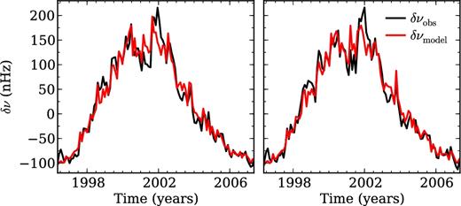
Comparison between the observed (black) and model (red) frequency shifts over the solar cycle 23 obtained using Samples 1 and 2 (left- and right-hand panel, respectively – see text for details).
A quasi-biennial variation with an 11-yr amplitude modulation was also identified by the authors in the residuals of the model-data comparison. This component, as well as the 11-yr variation, has been identified previously in data obtained from different space- and ground-based instruments and discussed in a number of works (cf. Section 1), while the shortest term component (varying on a time-scale of days) was first discussed in Paper I.
3 DESCRIPTION OF THE METHOD
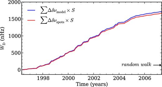
Weighted sum of the variations in the model (blue) and spot-induced (red) frequency shifts (derived from the observational sunspot data), where the weight S, in equation (2), is determined by the variation in the area covered by sunspots. The black arrow marks the expected standard deviation for a random walk.
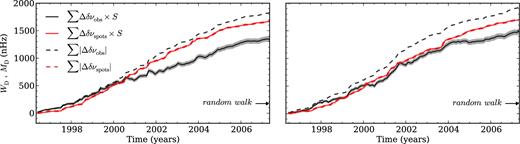
Left- and right-hand panels correspond to the results obtained for Samples 1 and 2, respectively. Weighted sum WD of the variation in the observed (black solid line) and spot-induced (red solid line) frequency shifts (derived from the observational sunspot data), where the weight, S, is determined by the variation in the total observed area covered by sunspots. The grey region represents the 1σ confidence interval from the black continuous curve resulting from the errors in the observed frequency shifts. The dashed lines represent the sum, MD, of the absolute (modulus) values of the frequency-shift differences. The arrow marks the expected standard deviation for a random walk.
We also verified to what extent the results for WD are affected by the error associated with the observed frequency shifts. By taking the observational data points and assuming that the corresponding errors are Gaussian, we obtain random samples for the frequency shifts. We then estimate the standard deviation from WD, which is represented by the grey area in Fig. 3. For some data points, the observational errors are of the same order as the frequency-shift differences. However, those data points do not contribute significantly to WD. Clearly, the uncertainty in the black curve (grey region) associated with the observational errors in the frequency shifts does not explain the loss of correlation found.
We thus conclude that a strong, but not complete correlation exists between the short-term variations in the frequency shifts and in the spots’ areas. The origin of the observed loss of correlation can be twofold: it may result from our inability to compute the true correlation between these two variations, or it may correspond to a genuine loss of correlation introduced either by changes in the effect that sunspots have on the frequencies or by the effect of other physical phenomena (besides spots), which may influence the solar frequency shifts on short time-scales. In the next section, we will discuss a potential source for that loss of correlation, associated with the lack of information about the sunspots on the invisible side of the Sun.
4 IMPACT OF IGNORING THE SOLAR INVISIBLE SIDE ON THE COMPUTATION OF WD
Even if a complete correlation existed between the variations in the frequency shifts and in the total area covered by spots, we would still expect to see a significant loss of correlation when comparing the quantities WD and MD derived from the observations. The reason is that the sunspot areas we consider for the computation of WD, obtained from the NGDC/NOAA data bases, concern only the visible sunspot groups, while the acoustic frequencies are affected by sunspot groups emerging over the whole solar surface. In this section, we estimate the effect of having ignored the invisible sunspot groups in the computation of WD of the previous section. To that end, we use synthetic sunspot data obtained with an empirical tool developed by Santos et al. (2015). This tool generates synthetic sunspot daily records analogous to the real sunspot data from NGDC/NOAA, starting from simulations of sunspot groups on both the visible and invisible sides of the Sun.
Using the model presented in Paper I, we compute the spot-induced frequency shifts for the synthetic sunspot data, δνsynthetic, taking into account all the spots, including those appearing on the visible and invisible sides of the Sun. Since the model for the frequency shifts is parametrized, it needs to be calibrated by comparison with the observed data. In this case, we are interested in analysing the short-term variations in the frequency shifts. We thus have calibrated the frequency shifts such as to make their absolute sum equal to the absolute sum of the observed counterparts, i.e. ∑k|Δδνobs|k = ∑k|Δδνsynthetic|k. We then compute WD for the synthetic data, by combining the variations in the frequency shifts obtained from all the synthetic sunspot groups with the weights Sk computed only from the visible synthetic sunspot areas. Since the sunspot cycle simulations are stochastic, we repeated this exercise 1000 times, computing the values of WD and MD for all simulations.
The quantities MD and WD derived from the synthetic data are shown in the top panel of Fig. 4 for one particular simulation. The difference between these quantities gives an estimate of the loss of correlation that can be explained by our not accounting for the sunspot groups on the invisible side of the Sun when computing the weights Sk. The bottom panel of Fig. 4 shows the distribution of that difference at the end of the solar cycle. Taking the average of the distribution as an indicator and comparing it with the difference between MD and WD computed in Section 3 for the observations, we conclude that only about 30 per cent of the loss of correlation found in the analysis of the real data may be explained by this non-physical effect. Therefore, a significant part of the loss of correlation detected in Section 3 is expected to have its origin in physical effects other than sunspots that affect the short-term frequency shifts and that are not, themselves, fully correlated with the total area covered by sunspots.
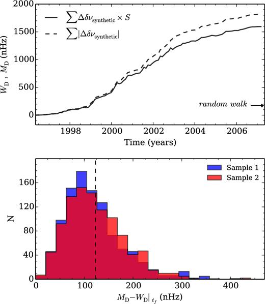
Top panel: comparison between the quantities MD (dashed line) and WD (solid line) for a particular synthetic cycle. The arrow marks the expected standard deviation for a random walk. Bottom panel: distribution of the difference between the quantities MD and WD at the end of the synthetic solar cycle (at tf). The dashed line marks the averaged difference found for both samples of independent frequency shifts.
5 EPOCHS OF DISTINCT BEHAVIOUR BETWEEN THE FREQUENCY SHIFTS AND THE SUNSPOT AREAS
While the frequency-shift differences are found to be strongly correlated with the variations in the area covered by sunspots, there are particular epochs when the frequency shifts and the sunspot areas vary in the opposite way, leading to the loss of correlation found in Section 3. In this section, we identify those epochs.
The top panels of Fig. 5 show the difference between MD (black dashed line in Fig. 3) and WD (black solid line in Fig. 3) for the observed frequency shifts. The results for the two samples differ slightly. For Sample 1 (left-hand panel), the differences have a larger amplitude around the solar maximum, while for Sample 2 they are more evenly spread. We recall that the two samples provide 36- d averages of the frequency shifts that are shifted by 18 d. The differences seen in the results for the two samples highlight that a significant loss of correlation takes place on shorter time scales than 18 d. In the discussion that follows we will, therefore, consider only aspects that are identified in both samples.
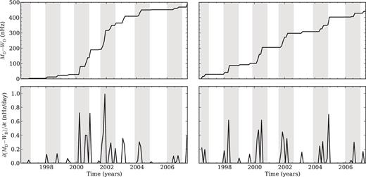
The left-hand panel concerns Sample 1, while the right-hand panel corresponds to Sample 2 (see text for details). Top panels: difference between the absolute sum, MD, and the weighted sum, WD, of the observed frequency-shift variations, i.e. between the black-dashed and solid lines in Fig. 3. Bottom panels: time derivative of the difference shown in the top panels. The grey bars, with a width of one year, are centred around the approximate location of the maxima of the quasi-biennial signal detected by Broomhall et al. (2012).
The bottom panels of Fig. 5 show the derivative of the difference between MD and WD with respect to the time. This quantity is zero when the variations in the frequency shifts have the same sign as those in the sunspot areas, differing from zero when the two variations have an opposite sign. The most significant correlation losses occur around the same times for the two samples of independent frequency shifts. The peaks are quasi-periodic, coinciding with the maxima of the quasi-biennial periodicity observed in the solar acoustic frequencies. This is illustrated by the grey bars in Fig. 5, which have a width of 1 yr and are centred at the locations of maxima of the quasi-biennial signal found by Broomhall et al. (2012).
6 DISCUSSION
Our results show that there is a strong correlation between the short-term variations in the frequency shifts and in the area covered by sunspots. However, the loss of correlation between the two is still significant and cannot be fully explained by the combined effect of the sunspot groups on the invisible side of the Sun and of the observational error in the observed frequency-shift differences. Moreover, the detailed analysis of the difference between the quantities WD and MD shows that opposite variations in the frequency shifts and in the sunspot area are more significant around the times of maxima of the quasi-biennial signal. This clear signature of the quasi-biennial variations in the quantity WD highlights the fact that the short time-scale variations are modulated on a quasi-biennial time-scale.
The above findings could point to a quasi-biennial change in the effect of the sunspots. However, we find this possibility difficult to understand on physical grounds because it would require that an increase in the sunspot area leads to a decrease in the frequency shifts at the maximum of the quasi-biennial variations. According to the model for the spot-induced frequency shifts (Paper I), this would imply that the phase shift induced by a sunspot on the acoustic wave travelling through it changed sign from the minimum to the maximum of the quasi-biennial variation. Another, perhaps more likely possibility is that other active-related features, such as plage, not accounted for in the computation of WD, could contribute to the short-term variations in the frequency shifts. However, given the asymmetry found between the behaviour of the correlations at the maximum and minimum of the quasi-biennial variations, their effect would have to dominate the short-term frequency-shift variations during the former, but be unimportant, compared to the effect of sunspots, during the latter. This possibility will be further investigated by inspecting the behaviour of 10.7-cm flux, discussed in the next subsection.
6.1 Short-term variations in the 10.7-cm flux
The acoustic frequency shifts are found to be better correlated with the 10.7-cm flux than with other activity proxies (e.g. Chaplin et al. 2007; Tripathy et al. 2007; Jain et al. 2009). Besides the contribution from sunspots, the 10.7-cm flux is also affected by radio plages and the quiet-Sun background in the upper chromosphere and lower corona (e.g. Covington 1969; Tapping 1987; Tapping & Detracey 1990). Given its sensitivity to both sunspots and plages, the 10.7-cm flux may provide a more complete picture of the short-term variations in the solar activity than the sunspot areas alone. To test this possibility, we repeated our analysis using the variations in the 10.7-cm flux (from NGDC/NOAA) instead of the sunspot area variations as the weight in equation (2). The results, shown in Fig. 6, confirm that the loss of correlation is less pronounced in this case than when the sunspot area variations are used (around 40 per cent smaller than that found in Figs 3 and 5). Despite this, we still find that, in general, the loss of correlation is more significant around the maxima of the quasi-biennial variations.
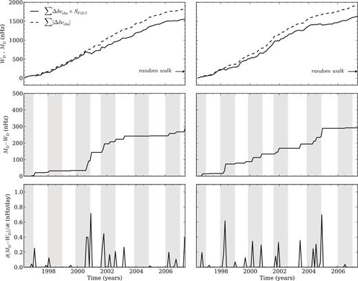
The left-hand panel concerns Sample 1, while the right-hand panel corresponds to Sample 2. Top panels: weighted sum of the variations in the observed frequency shifts (black solid line), where the weight S, in equation (2), is determined by the variation in the 10.7-cm flux. The dashed line represents the sum of the absolute (modulus) values of the frequency-shift differences, MD. Middle panels: difference between the dashed and solid lines in the top panels. Bottom panels: derivative of the difference shown in the middle panels. The grey bars, with a width of one year, are centred around the approximate location of the maxima of the quasi-biennial signal detected by Broomhall et al. (2012).
The comparison between the results found for the area covered by sunspots and for the 10.7-cm flux confirms that the latter contains contributions from additional activity-related features (besides sunspots) that vary on short time-scales and that these features have a significant impact on the short-term variations of the frequency shifts. Moreover, we may conclude from the results for the 10.7 cm that spots and plages alone do not fully explain the short-term variations in the observed frequency shifts.
7 CONCLUSIONS
In this work we investigated the correlation between the variation in the solar frequency shifts and in the area covered by sunspots. In particular, we proposed a new observable, consisting in the sum of the frequency shifts weighted by the variation of the sunspot area, which isolates and amplifies the signal from the short-term variations in the frequency shifts. Using this new observable, we found a strong correlation between the short-term variations in the area covered by sunspots and in the frequency shifts. Nevertheless, a significant loss of correlation is still observed, generally coinciding with the times of maxima of the quasi-biennial variations seen in the solar acoustic frequencies. The loss of correlation on short time-scales suggests that other physical phenomena, besides sunspots, acting on time-scales shorter than 36 d contribute to the frequency shifts and that their relative importance changes in phase with the quasi-biennial signal.
We also considered the case in which the variation of the 10.7-cm flux, rather than the visible sunspot area, is used as a weight in the computation of the new observable. The short-term variation in the frequency shifts was found to vary even more closely in line with the 10.7-cm flux than with the sunspot areas, confirming that the 10.7-cm flux contains information about additional activity-related features which contribute to the frequency shifts. Nevertheless, a significant loss of correlation, whose physical origin remains to be fully understood, is again observed around the times of maxima of the quasi-biennial signal.
Acknowledgments
This work was supported by Fundação para a Ciência e a Tecnologia (FCT) through the research grant UID/FIS/04434/2013. ARGS acknowledges the support from FCT through the Fellowship SFRH/BD/88032/2012 and from the University of Birmingham. MSC and PPA acknowledge support from FCT through the Investigador FCT Contract numbers IF/00894/2012 and IF/00863/2012 and POPH/FSE (EC) by FEDER funding through the programme Programa Operacional de Factores de Competitividade (COMPETE). TLC and WJC acknowledge the support of the UK Science and Technology Facilities Council (STFC). The research leading to these results has received funding from EC, under FP7, through the grant agreement FP7-SPACE-2012-312844 and PIRSES-GA-2010-269194. ARGS, MSC, and PPA are grateful for the support from the High Altitude Observatory (NCAR/UCAR), where part of the current work was developed.
A similar comparison was shown in Paper I, but for the two data sets combined.
