


In the Λcold dark matter model of structure formation, a stellar spheroid grows by the assembly of smaller galaxies, the so-called building blocks. Combining the Munich–Groningen semi-analytical model of galaxy formation with the high-resolution Aquarius simulations of dark matter haloes, we study the assembly history of the stellar spheroids of six Milky Way-mass galaxies, focusing on building block properties such as mass, age and metallicity. These properties are compared to those of the surviving satellites in the same models. We find that the building blocks have higher star formation rates on average, and this is especially the case for the more massive objects. At high redshift, these dominate in star formation over the satellites, whose star formation time-scales are longer on average. These differences ought to result in a larger α-element enhancement from Type II supernovae in the building blocks (compared to the satellites) by the time Type Ia supernovae would start to enrich them in iron, explaining the observational trends. Interestingly, there are some variations in the star formation time-scales of the building blocks amongst the simulated haloes, indicating that [α/Fe] abundances in spheroids of other galaxies might differ from those in our own Milky Way.
1 INTRODUCTION
The formation and evolution of the Galactic spheroid, consisting of the central bulge and the stellar halo, has been studied for more than 50 yr since the classical paper of Eggen, Lynden-Bell & Sandage (1962) on the origin of the Milky Way. Although it is still unclear to which extent accretion plays a role besides instabilities of the disc in the formation of the Galactic bulge (e.g. Combes 2000; Gerhard 2015; Di Matteo 2016), there is growing consensus on the formation of the Galactic halo. Since the proposed scenario of Searle & Zinn (1978) in which the stellar halo formed via the merging of several protogalactic clouds, there have been many pieces of evidence suggesting indeed a hierarchical build-up of the Milky Way's stellar halo (e.g. Ibata, Gilmore & Irwin 1994; Helmi et al. 1999; Belokurov et al. 2006; Bell et al. 2008; Starkenburg et al. 2009; Janesh et al. 2016). Presently, we have a firm theoretical framework provided by the Λcold dark matter paradigm predicting a hierarchical formation scenario that can be simulated in much detail (e.g. Johnston 1998; Bullock, Kravtsov & Weinberg 2001; Bullock & Johnston 2005; Abadi, Navarro & Steinmetz 2006; Moore et al. 2006). On the other hand, the accretion history of our Galaxy in particular is not completely unravelled yet, although much progress is expected thanks to the Gaia mission (Perryman et al. 2001). One particularly intriguing question is how the building blocks that formed our Milky Way's accreted spheroid compare to the satellite galaxies that we see around us today.
In a pioneering paper, Unavane, Wyse & Gilmore (1996) attempted to constrain the accretion history of the stellar halo from comparisons of the age distribution and chemical abundances of halo stars with those of the stars in present-day dwarf spheroidal (dSph) galaxies. Numerous observational studies (Shetrone, Bolte & Stetson 1998; Shetrone, Côté & Sargent 2001; Shetrone et al. 2003; Tolstoy et al. 2003; Venn et al. 2004; Koch et al. 2008; Tolstoy, Hill & Tosi 2009; Kirby et al. 2010) reported discrepancies between chemical abundances of satellite galaxies of the Milky Way and field halo stars. These studies show that the present-day satellites are, at least partly, unlike the building blocks of the Milky Way's stellar spheroid. The dSphs that we see around the Milky Way in our Local Group are survivors and thus had naturally more time to form stars than the building block galaxies that already dissolved into the halo (e.g. Mateo 1996). Even when comparing equal age populations in both environments (as done by Fiorentino et al. 2015, using RR Lyrae stars), discrepancies are found between the typical dSphs that survived and those that contributed majorly to the build-up of the spheroid.
In this work, we specifically focus on the properties (in terms of mass, age and metallicity) of the building blocks of our Milky Way's accreted spheroid modelled within a fully cosmological framework. We investigate when they merged and how they relate to the surviving satellite population. In the past decade, several efforts have already focused on the build-up of Milky Way stellar haloes and/or their chemical evolution, either using hydrodynamical simulations or with semi-analytic techniques (e.g. Bullock & Johnston 2005; Tumlinson 2006, 2010; Salvadori, Schneider & Ferrara 2007; Zolotov et al. 2009; Cooper et al. 2010, 2015; Font et al. 2011; Tissera et al. 2013; Pillepich et al. 2014; Tissera et al. 2014; Lowing et al. 2015; Pillepich, Madau & Mayer 2015). A specific focus on chemical evolution has been provided by Robertson et al. (2005)and Font et al. (2006a,b), using the hybrid semi-analytic plus N-body approach of Bullock & Johnston (2005). Cooper et al. (2010, hereafter C10) used the galform semi-analytic galaxy formation model to study the disruption of satellite galaxies within the cosmological N-body simulations of the six galactic haloes of the Aquarius project (Springel et al. 2008), which have masses comparable to values typically inferred for the Milky Way halo.
We use here a different semi-analytic model to study the formation of our Galaxy and its spheroids’ building blocks than C10 (Starkenburg et al. 2013a, hereafter S13, and references therein), but using also the Aquarius simulations as a backbone. In Section 2, we briefly describe our model, followed by a detailed description of the resulting stellar spheroids in Section 3. We will focus on their accreted components, but in this section, we will also show how they relate to the full spheroids in terms of stellar mass. In Section 4, we investigate the stellar mass–metallicity relation for the building blocks of the accreted spheroids and compare this to the observed stellar mass–metallicity relation for the surviving satellite galaxies of the Milky Way, and the simulated one by S13. In this section, we also show that the early star formation (i.e. over 12 Gyr ago) in the accreted spheroid was dominated by its building blocks and was much lower in the satellite galaxies that survive until the present day. We apply our analysis to infer observable [α/Fe] trends in galaxies with various accretion histories in Section 5 and we conclude in Section 6.
Throughout this paper, we name all accreted stellar material together the ‘accreted spheroid’ of a galaxy. This definition is preferred over the term ‘halo’ to clarify that this component is present at all radii. Only in Section 3, we furthermore use the term ‘accreted bulge’ for the innermost 3 kpc of the accreted spheroid.
2 THE MODEL
We use the semi-analytic model for galaxy formation that was originally established in Munich (Kauffmann et al. 1999; Springel et al. 2001; De Lucia, Kauffmann & White 2004; Croton et al. 2006; De Lucia & Blaizot 2007; De Lucia & Helmi 2008) and developed further in Groningen (Li, De Lucia & Helmi 2010, S13). The merger history trees of the six Milky Way-like haloes of the Aquarius project, denoted A–F (Springel et al. 2008), and their substructures were constructed using the subfind algorithm (Springel et al. 2001), after which baryonic processes are modelled using simple but observationally and astrophysically motivated prescriptions (De Lucia et al. 2004; Li et al. 2010, S13 and references therein).
A galaxy merger tree was constructed to follow the galaxies that end up in the Milky Way's stellar spheroid over time. Each building block of the spheroid undergoes three phases in this galaxy merger tree: a first phase where it is a main galaxy with its own dark matter halo; a second phase where it is a satellite galaxy (its dark matter halo becomes a subhalo of a more massive halo); and a so-called orphan phase, where the dark halo of a satellite galaxy is tidally stripped down to below the subfind resolution limit of 20 particles. Up until this last point, where the galaxy has ‘lost’ its dark matter halo, the galaxy merger tree is identical to the dark matter merger tree.
Despite the semi-analytical nature of our model in which no stellar particles are explicitly modelled or tagged, our model includes some prescription of stellar stripping in merging satellites, but only when the dark matter halo of a satellite galaxy is so heavily stripped that its half-mass radius becomes smaller than the half-mass radius of the stars and cold gas. In this case, the stars and cold gas are removed up to the half-mass radius of the dark matter and added to the host spheroid (see S13, appendix A1). Orphan galaxies – a class that is particularly difficult to handle well, because no information on them is present in the simulations anymore – either merge with the central galaxy on a dynamical friction time-scale before redshift zero, or, if this time-scale is longer, might survive. In the latter case, their survival depends on their average mass density compared to that of their host system (see S13, appendix A2). We note that besides stripping of their dark matter mass and possibly some stellar content, surviving orphan galaxies are similar to any surviving dwarf galaxy including a chemical history of self-enrichment (which sets them apart from globular clusters for instance; Kruijssen et al. 2012; Leaman 2012; Willman & Strader 2012). Some fainter orphan galaxies could potentially even still be dark matter dominated. Note that the tidal disruption of orphan galaxies is another way of growing the spheroid, as is stellar stripping.
To summarize, the five ways of spheroid growth in our model are: (1) major mergers, (2) minor mergers on a dynamical friction time-scale, (3) disc instabilities, (4) stellar stripping and (5) tidal disruption of orphans. The four different types of galaxies that we model are: (1) main galaxies that do survive until the present day. These galaxies have a dark matter halo and may have several satellite galaxies in subhaloes of this dark halo or orphan galaxies bound to them. The most massive of these main galaxies in our simulation is our model Milky Way. (2) Building block galaxies that once were main galaxies but went through the above-mentioned three phases of evolution before merging with our progenitor Milky Way galaxy. These do not survive until the present day. (3) Surviving satellite galaxies of a main galaxy, which do have a dark matter halo that is a subhalo of the dark halo containing the main galaxy. (4) Orphan galaxies that might eventually merge with a main galaxy but survive until the present day.
Our model assumes an instantaneous recycling approximation, i.e. we do not take into account finite stellar lifetimes. The abundance of an α-element such as Mg for instance, mainly originating in short-lived supernovae (SNe) Type II, can therefore better be compared with the metallicity predicted by our model than Fe, which is thought to originate mainly in the (delayed) population of Type Ia SNe. No individual elements are explicitly traced in the model though, instead it returns a total mass in metals for any system in the gas and stars. Throughout this paper, we refer to the metallicity of any stellar system by | $\log [\mathrm{{\rm {\it Z}}}_\mathrm{stars}/\mathrm{Z}_{\odot }]$ |, i.e. the logarithm of the ratio of mass in metals over the total mass in stars in that galaxy, divided by the solar metallicity, Z⊙ = 0.02. Two discrepancies, however, arise when comparing this modelled metallicity with observational data: (1) often, in observational data, [Fe/H] is measured, rather than [Mg/H] and (2) the average [Fe/H] of a stellar system is calculated by taking the average of the logarithms of (a representative sample of) its individual stars’ iron abundance ratios compared to that of the Sun, whereas we take the logarithm of the average metallicity compared to that of the Sun. Thus, the metallicity values that we find are higher. In our comparisons with data, we attempt to compensate for both discrepancies. We refer the reader to S13 for details (i.e. see their equation 2 and the paragraph below that equation), but in short, we convert each measured [Fe/H] into [Mg/H] and apply an offset to correct for the difference in the averaging procedure.
3 THE STELLAR SPHEROIDS
Our modelled stellar spheroids are part of galaxies that were already analysed in some detail in S13, who looked at the total stellar mass of the galaxies that developed in the six Aquarius haloes as well as their bulge/disc ratios. As pointed out by S13, if viewed as one component, the integrated or average values for the spheroids can best be compared with the Milky Way bulge since the stellar halo contains very few stars compared to the bulge. In terms of metallicity, spheroid B has the closest match to the observed bulge metallicity of the Milky Way of [Fe/H] ∼ −0.25 (McWilliam & Rich 1994; Zoccali et al. 2003; Bensby et al. 2013). S13 found that the bulge/disc ratios of the simulated galaxies in all Aquarius haloes except E and F are close to the estimated value of 0.2–0.3 (Bissantz, Debattista & Gerhard 2004) for the Milky Way. We list the disc stellar mass and the spheroid stellar mass in Table 1. The simulated galaxies in Aquarius haloes B and E are the closest Milky Way analogues in terms of total stellar mass, i.e. the sum of these first two columns.
The stellar mass of the disc, total spheroid stellar mass, the accreted spheroid stellar mass, the fraction of accreted spheroid stellar mass contributed by surviving satellite galaxies fsurv, the percentage of surviving satellites that are orphan and the number of significant progenitors Nprog, per halo.
| Halo | M*, disc | M*, sph. | M*, acc. | fsurv | orph | Nprog |
|---|---|---|---|---|---|---|
| | ${}_{10^{10} \,\mathrm{M}_{\odot }}$ | | | ${}_{10^{10} \,\mathrm{M}_{\odot }}$ | | | ${}_{10^{10} \,\mathrm{M}_{\odot }}$ | | ( per cent) | |||
| A | 15.35 | 3.409 | 0.467 | 0.104 | 36 | 3.3 |
| B | 5.925 | 1.080 | 0.896 | 0.034 | 23 | 3.1 |
| C | 15.79 | 4.906 | 0.529 | 0.482 | 45 | 6.1 |
| D | 12.40 | 3.431 | 1.182 | 0.484 | 32 | 5.4 |
| E | 3.156 | 1.932 | 1.305 | 0.009 | 35 | 1.3 |
| F | 5.182 | 3.890 | 1.226 | 0.896 | 31 | 1.4 |
In Fig. 1, we show the growth of the six Aquarius spheroids over time, including the stars that were moved to the spheroid through disc instability (solid lines) or excluding this and showing the contribution from accreted stellar mass only (dashed lines). The final spheroid masses can be read off from the vertical axis of each panel (and are listed in Table 1). They vary from 1.1 × 10¹⁰ M⊙ for spheroid B to 5.2 × 10¹⁰ M⊙ for spheroid C. Whereas spheroid B grows more gradual, the other Aquarius spheroids have undergone one or two major growths. Interestingly, whereas Aquarius haloes B and E contain the least massive galaxies in terms of total stellar mass (S13), they have the largest fraction of accreted spheroid stars compared to their total spheroid mass, since the contribution of disc instabilities to the build-up of the total spheroid is smallest in these haloes. The fraction is smallest in Aquarius haloes A and C, which also have the lowest accreted stellar mass in an absolute sense. Whereas the disc instability channel is mainly considered to lead to the formation of the galactic bar that is much more centrally concentrated, accreted material will contribute at all radii. The largest mass ratio (mass in stars and cold gas) that we find for galaxies merging with the central galaxy in our simulation is 0.23. Because we assign the label major only to a merger in which this ratio is larger than 0.3, none of the Milky Way galaxies in our simulations have undergone a major merger during their lifetimes, and even their mergers with the most massive building blocks are classified as minor. Consequently, we do not find any stars that were formed in situ in our spheroids, since in situ star formation only happens in major mergers in our model.
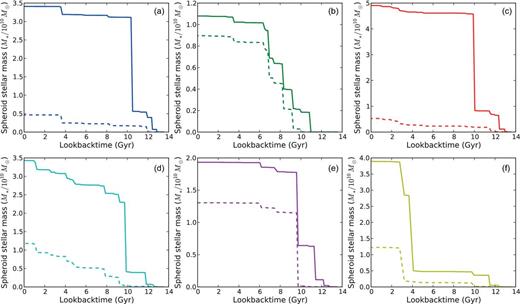
Build-up of the six Aquarius spheroids in stellar mass over time. Solid lines indicate the full spheroid growths, including stars that were moved from the disc to the spheroid by the disc instability channel (see Section 2). Dashed lines indicate the spheroid growth by accretion only.
In Table 1, the stellar masses of these accreted spheroids are listed, as well as the fraction of the accreted spheroid stellar mass that is material stripped from surviving satellites fsurv. This fraction is very large for Aquarius halo F, because the progenitor that almost completely accounts for its spheroids total stellar mass has a still surviving counterpart. For Aquarius haloes C and D, we also find large values of fsurv, which is in agreement with the result from C10. The difference between our results and those of C10 – in particular for halo F, but in lesser extent for the other haloes – is probably due to our differences in the treatment for the tidal disruption of orphan galaxies and stellar stripping (C10 make use of a particle tagging technique).
Table 1 also lists the percentage of surviving satellites that is orphan, when using the S13 prescriptions that we summarized in Section 2. We see that they constitute ∼1/3 of the total population of surviving satellites in most haloes.
The stellar mass of the accreted spheroids is on average 9.3 × 10⁹ M⊙ in our models. The resulting accreted spheroid/disc mass ratios that we find are 0.03, 0.15, 0.03, 0.10, 0.41 and 0.24 for haloes A–F respectively. Using the same Aquarius haloes but a different semi-analytic model, C10 find, on average, accreted spheroids of 1.2 × 10⁹ M⊙, thus, on average, almost a factor of 8 lower. To find differences between the two codes in these values is not so surprising; the stellar mass–halo mass relation in our model is quite different from that in galform in this mass range due to their stronger feedback (see S13 for a discussion).
On average, 38 per cent of the accreted spheroid stars in the galform semi-analytic model of C10 is located in the innermost 3 kpc. They refer to this component as the accreted bulge. The spread between these fractions in the six Aquarius haloes is large within their model, i.e. 26, 59, 8.7, 12, 90 and 20 per cent for haloes A–F, respectively. Since we have no particle tagging scheme implemented, we cannot make this distinction based on distances in our models, however, if the accreted spheroid stars in our model were distributed among bulge (inner 3 kpc) and halo according to the percentages derived from C10, the accreted stellar haloes (excluding the accreted bulge) A–F would respectively be 3.4, 3.6, 4.8, 10, 1.2 and 9.7 × 10⁹ M⊙ in our model. Aquarius halo E, containing the lowest mass galaxy, also contains the lowest mass stellar halo. Note that this estimate of its stellar halo mass matches our analytical estimate above.
The rightmost column in Table 1 lists the number of significant progenitors Nprog of the accreted spheroids. Following C10, this number is defined as | $N_\mathrm{prog} = M_{\mathrm{tot},*}^2/\sum _i m_{\mathrm{prog},i,\ast}^2$ |, which is the total number of progenitors in the case where each contributes equal mass, or the number of significant progenitors in the case where the remainder provide a negligible contribution. mprog, i, * is the total stellar mass of a building block, or the total stellar mass stripped from one and the same surviving satellite. The sum of all progenitor masses thus equals the total accreted stellar mass of the spheroid (∑improg, i, * = Mtot, *). While the full spheroids (including the disc instability mechanisms) are dominated by one or two major growths only, as shown in Fig. 1, we see from Table 1 that the accreted spheroids are typically built out of several significant building blocks.
We find that the stellar spheroid is built almost completely by a few main progenitor galaxies, as C10 find for the stellar halo. However, the number that we find is for all Aquarius haloes, except halo A, higher than the result of C10, most significantly for halo C (for which they find Nprog = 2.8), although only marginally for haloes E and F. For halo C, we find nine building blocks with a stellar mass larger than 108 M⊙, which is more than in any of the other Aquarius haloes, and indeed points to a large number of significant progenitors, even though the total accreted mass of this spheroid is one of the lowest (see Table 1). Our accreted spheroids B, E and F have the lowest number of progenitors, in agreement with C10's finding that the accreted haloes corresponding to these Aquarius haloes have the lowest Nprog. The larger number of significant progenitors that we find for haloes B, C and D could be due to our different selection of radii, i.e. C10 do not include any stars within a 3 kpc distance from the Galactic Centre in their halo selection. The other differences between our model and that of C10 that could again play a role are the different stellar mass–halo mass relation and the treatment of stellar stripping and the tidal disruption of orphan galaxies.
Fig. 2 shows the spheroids’ star formation rates (SFRs, in M⊙ yr−1) as a function of lookback time. The six black solid lines in Fig. 2 show the total SFRs of the accreted spheroids, i.e. the sum of the SFRs of all building blocks. With dashed, dotted, dot–dashed and coloured solid lines, the SFRs of the main progenitor galaxies are shown. These main progenitors were selected to contribute at least 10 per cent of the spheroid's stellar mass. Note that this selection criterion is more simplistic than the non-integer statistical count of main progenitors as defined in C10 and presented in Table 1. The blue dashed lines represent the SFRs of the most massive progenitor galaxies, the green dotted lines the second most massive progenitors, red dot–dashed the third and cyan solid lines the fourth (if applicable). Most of these main progenitors are completely disrupted, but for haloes C, D and F, respectively, 69 per cent, 94 per cent and 54 per cent of the original stellar mass of a still surviving satellite constitute its most massive ‘building block’.
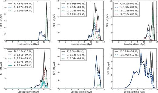
Star formation rates of the accreted spheroids (black solid lines), in combination with the star formation rates of their main progenitor galaxies, i.e. the largest building blocks (dashed, dotted and dot–dashed lines) that contribute to them. These main progenitors were selected to contribute at least 10 per cent of the spheroid's stellar mass. The first number in the legend of each panel is again the total accreted stellar mass of that spheroid, followed by the stellar mass of the largest building blocks.
In Fig. 3, we show the ages (in bins of 1 Gyr) and metallicities (| $\log [\mathrm{{\rm {\it Z}}}_\mathrm{stars}/\mathrm{Z}_{\odot }]$ |, in bins of 0.5 dex) of the accreted spheroids. The stars in the lowest luminosity bin (| $\log [\mathrm{{\rm {\it Z}}}_\mathrm{stars}/\mathrm{Z}_{\odot }]< -6$ |) in Fig. 3 were formed without any metals; these (still) exist in our model due to the neglection of any kind of pre-enrichment from Population III stars in our model. The majority of our modelled accreted stellar spheroid population have near-solar metallicity abundances. This is in agreement with the observed average [Mg/H] value for bulge stars, eg. [Fe/H] ∼−0.25 (McWilliam & Rich 1994; Zoccali et al. 2003; Bensby et al. 2013), which combined with [Mg/Fe] ∼+0.25 brings the observed average [Mg/H] to solar. However, it is difficult to compare our model, which predicts the metallicity distribution function of spheroid stars over all radii, directly to an observed one (eg. An et al. 2013; Allende Prieto et al. 2014), because the observations are made in a certain direction and/or distance range. If we interpret the lower metallicity accreted spheroid stars as halo stars, we seem to underestimate the lowest metallicities (<∼ −2) compared to the observed distributions by An et al. (2013) and Allende Prieto et al. (2014).
![Age–metallicity Maps ( $\log [\mathrm{{\rm {\it Z}}}_\mathrm{stars}/\mathrm{Z}_{\odot }]$ ) of the six accreted spheroids. The colour map represents the stellar mass (M⊙) per bin, on a logarithmic scale. In the bottom left corner of each panel, the total accreted stellar mass of that spheroid is indicated.](https://oup.silverchair-cdn.com/oup/backfile/Content_public/Journal/mnras/464/1/10.1093_mnras_stw2340/4/m_stw2340fig3.jpeg?Expires=1750502186&Signature=fyJUhzq7GEflafuUIlYwJtBbSY7zMHj9g2qCEjcYGOW0xT6fbPKDWLu6VQuRzGMVNdyOg-tiOugPp0rl4f6ASitq-7T6AYe8zwB0b3aFW8k93PAHl1jpWkt6jxcqhZebWBXLCzlzhKsHmUahclsaXSmV6ONFAoM50of5zHj4g9ub93LPlI7XSNnUaqg7pGOKXkZJO58bCVUKKrjdmHaOI12rH19WhQ5rjEzE8-hxoyuFakHbAi30CEXjvvx~8-0XPeVU7ahJv926fVX-~aI2Wyl-QEN0GmdNTKEUj1FFGJU9nXOT6bJvFTBKpEZc4FW3choxTgGU19cuivyl0F8YRg__&Key-Pair-Id=APKAIE5G5CRDK6RD3PGA)
Age–metallicity Maps (| $\log [\mathrm{{\rm {\it Z}}}_\mathrm{stars}/\mathrm{Z}_{\odot }]$ |) of the six accreted spheroids. The colour map represents the stellar mass (M⊙) per bin, on a logarithmic scale. In the bottom left corner of each panel, the total accreted stellar mass of that spheroid is indicated.
From Figs 2 and 3, it is clear that the majority of spheroid stars is old. An exception is the stellar spheroid of F, but this galaxy is atypical as a Milky Way analogue because its spheroid was built mainly by the recent stripping of stars from one still surviving (orphan) satellite, i.e. 3 Gyr ago (see the bottom right panel of Fig. 1).
As expected, our total spheroid's SFR values are very similar to those presented in fig. 8 in De Lucia et al. (2014) who use a slightly different version of the same semi-analytic code. Spheroid F looks very different between both models, but this is mainly due to the single massive progenitor galaxy mentioned above that either is counted as part of the Galactic spheroid (in our model) or not (in their model). In the corresponding erratum, De Lucia et al. (2015) moreover show that when they apply a new technique to account for finite stellar lifetimes in their model, rather than relying on an instantaneous recycling approximation, the total spheroid masses are typically lower by a factor of ∼2. The implementation of finite stellar lifetimes does also have a significant effect on their overall spheroid metallicity; these are typically lowered by ∼0.5 dex.
4 COMPARISON OF BUILDING BLOCKS AND SURVIVING SATELLITES: METALLICITY AND SFR
Having presented the SFRs of the most massive building blocks in the previous section and Fig. 2, we will now discuss in more detail the properties of all the building block galaxies and compare them with those of the surviving satellites. We would like to point out that although the number of building blocks is smaller than the number of surviving satellites (for spheroid E the number of building blocks is even less than half the number of surviving satellites), the total stellar mass in building blocks is much larger than the stellar mass in surviving satellites for most spheroids, for spheroid B even more than a factor of 10. The exceptions are spheroid A (where the stellar mass is similar in the two populations) and spheroid F (which has more mass in surviving satellites).
In their fig. 5, S13 showed the luminosity–metallicity relation for the satellite galaxies of all Aquarius haloes and concluded from a comparison with observed average [Mg/H] values for the Milky Way satellites that the model resembles reality quite accurately. An exception are the model galaxies with metallicities <−3. Many more of those are seen in the models than we observe around the Milky Way. However, as explained in S13, these typically have experienced star formation in less than four snapshots of our simulation, resulting in a clear signature of the neglect of pre-enrichment from the very first generation of stars. All stars formed in the first star formation event are modelled to have no metals at all and an identical initial mass function (IMF) to more metal-rich components. A different, more top-heavy IMF for these first stars is, however, likely to enrich these galaxies easily to a metallicity floor of [Fe/H] ∼−3 (e.g. Salvadori, Ferrara & Schneider 2008).
In Fig. 4, we show the average metallicities (| $\log [\mathrm{{\rm {\it Z}}}_\mathrm{stars}/\mathrm{Z}_{\odot }]$ |) of these satellites (blue circles), as a function of their stellar mass and compare their values to those of the fully disrupted building blocks of the spheroids (yellow squares). The satellites/building blocks with less than or equal to four star formation snapshots (SFS) are plotted with open symbols in Fig. 4. These indeed cover almost all galaxies below metallicities <−3. Because of the neglect of pre-enrichment from the very first generation of stars, we do not trust the physical nature of the second line at metallicities ∼−4 below the physical mass–metallicity relation which is starting at metallicities ∼−2 (almost all symbols on this line are open). All satellites shown here are those within a 280 kpc radius from the centre of the central galaxy in our simulations, which is a proxy for the virial radius of the Milky Way (Koposov et al. 2008). Only a few satellites that are still bound to the central galaxy in our simulations can be found outside of this radius. Observed Milky Way satellites [Mg/H] values, corrected to better compare with our model calculations (as described at the end of Section 2) within the same radius are plotted as red triangles with error bars, which, for most galaxies, fall within the symbol size. Values are taken from McConnachie (2012).
![Stellar mass versus metallicity ( $\log [\mathrm{{\rm {\it Z}}}_\mathrm{stars}/\mathrm{Z}_{\odot }]$ ) relation for the building blocks (yellow boxes) and for the surviving satellites (blue circles). Building blocks/surviving satellites with more than four snapshots during which there is star formation (star formation snapshots, or SFS) are shown with filled marker symbols, those with less than or equal to four SFS with open symbols. The 88 ‘building blocks’ that are stripped material of a surviving satellite (17 per cent of the total number of BBs) are not shown. With a grey zone, we indicate what mass range of the building blocks/surviving satellites we do not trust due to the limiting resolution of our simulation. Observed satellite metallicity values (McConnachie 2012), corrected to approximate a mass-weighted average of [Mg/H] for a better comparison to the models (see the text for details) are plotted as red triangles with error bars. The seven points in the grey area correspond to Leo IV, Bootes III (which nature is unclear), Ursa Major (I), Leo V, Pisces II, Canes Venatici II and Ursa Major II, from right to left, respectively.](https://oup.silverchair-cdn.com/oup/backfile/Content_public/Journal/mnras/464/1/10.1093_mnras_stw2340/4/m_stw2340fig4.jpeg?Expires=1750502186&Signature=Gg-XPO0AD~26FmTb-gFVpHY3XhfjoEcB8oQgdQYV2JTJIgc9JOFEmiOBZCAL6LhCgqxdMGGw8FcOpt~DPH-HFY~bHH0Tyc7dGl2rC9OMRvkNoekPRQ~YIE4rq1zEf2JjU1lLTm4syaFN5m0Nh7BT0NxtBQABE4AfdjaSvLFH6Ud8rqz4AG0z~xq7~kCa32mIfZ8DoSNn4jbgour-ow2fXEd2GfAN~8kx1U2Bxs8laZQdemGxdnn1fBjWgltDvQvRSLFa4hY8RBqwHCRvpd~LHMtHCrwywPWCVCmZiJEDDTT5bJeXZbvZiKTfnadKCgKbuJwluBU02bqg0KrJ20iprw__&Key-Pair-Id=APKAIE5G5CRDK6RD3PGA)
Stellar mass versus metallicity (| $\log [\mathrm{{\rm {\it Z}}}_\mathrm{stars}/\mathrm{Z}_{\odot }]$ |) relation for the building blocks (yellow boxes) and for the surviving satellites (blue circles). Building blocks/surviving satellites with more than four snapshots during which there is star formation (star formation snapshots, or SFS) are shown with filled marker symbols, those with less than or equal to four SFS with open symbols. The 88 ‘building blocks’ that are stripped material of a surviving satellite (17 per cent of the total number of BBs) are not shown. With a grey zone, we indicate what mass range of the building blocks/surviving satellites we do not trust due to the limiting resolution of our simulation. Observed satellite metallicity values (McConnachie 2012), corrected to approximate a mass-weighted average of [Mg/H] for a better comparison to the models (see the text for details) are plotted as red triangles with error bars. The seven points in the grey area correspond to Leo IV, Bootes III (which nature is unclear), Ursa Major (I), Leo V, Pisces II, Canes Venatici II and Ursa Major II, from right to left, respectively.
Fig. 4 does not evidence much difference in the metallicities of the building blocks and those of the surviving satellites at a given stellar mass. In order to see if the two populations could be drawn from the same underlying distribution, we conducted a Kolmogorov–Smirnov (KS) test, thereby excluding the open symbols and the galaxies in the shaded areas, where we suspect the resolution of our simulation to limit the robustness of our results. Furthermore, we removed the mass dependence of the | $\log [\mathrm{{\rm {\it Z}}}_\mathrm{stars}/\mathrm{Z}_{\odot }]$ | values by subtracting a quadratic polynomial fit from the data: | $\log [\mathrm{{\rm {\it Z}}}_\mathrm{stars}/\mathrm{Z}_{\odot }]= ax^2 + bx + c$ | with x = log (Stellarmass /M⊙), a = −0.0208, b = 0.682 and c = −4.79. The resulting D statistic of 0.09 and p-value of 0.38 indicate that the populations are consistent with each other. For this case, we conclude that the two populations follow the same underlying distribution.
Fig. 5 shows the average SFR (in M⊙ yr−1) versus stellar mass, with the same colour coding as Fig. 4. We have calculated the average SFR as the sum of the SFRs prior to infall into the halo of a larger galaxy (i.e. the galaxy was not yet a satellite) divided by the total number of timesteps during which there was star formation in this period.
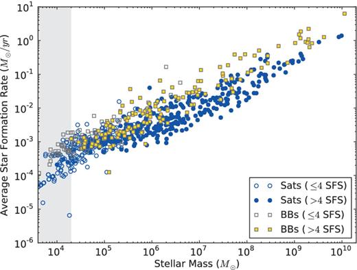
Stellar mass versus the average star formation rate for the building blocks (yellow boxes) and for the surviving satellites (blue circles). Building blocks/surviving satellites with more than four SFS are shown with filled marker symbols, those with less than or equal to four SFS with open symbols. The 88 ‘building blocks’ that are stripped material of a surviving satellite (17 per cent of the total number of BBs) are not shown. With a grey zone, we indicate what mass range of the building blocks/surviving satellites we do not trust due to the limiting resolution of our simulation.
It is clear from Fig. 5 that the average SFRs of the building blocks are typically higher at a given stellar mass than those of the surviving satellites. To quantify this difference, we again conducted a KS test on the two populations (open symbols, non-shaded area only) after subtracting a quadratic polynomial fit to remove the mass dependance of the SFR values: y = ax2 + bx + c with x = log(stellar mass/M⊙), y = log(average SFR/( M⊙ yr−1)) a = 0.0479, b = −0.0509 and c = −3.83. We find a D statistic of 0.49 and a p-value of 2.7 × 10⁻²². To check the sensitivity of this strong result on our choices of calculating the average SFRs described earlier, we additionally calculate the averages in various different ways: the sum of the SFRs in all timesteps during which there is star formation divided by the number of timesteps in which there is star formation (D: 0.51, p-value: 4.0 × 10⁻²⁴); and the total stellar mass of the building block/satellite divided by the timespan of star formation (D: 0.64, p-value: 5.7 × 10−37). Furthermore, we compared the peak SFRs of the building blocks and the surviving satellites, which show the same trend again (D: 0.49, p-value: 8.0 × 10⁻²³). Because the p-value is very low in all of these cases, we are convinced that our conclusion that the SFR in the building block population is higher than that in the surviving satellites is robust.
The left-hand panel of Fig. 6 shows the SFR of all fully disrupted building blocks weighted by their stellar mass at that time of star formation, versus the mass-weighted SFR of the surviving satellites, calculated separately for five of the Aquarius haloes, after which the median is plotted with a black line for the building blocks and with a blue line for the satellites. With a coloured band, the 30–70 percentiles are shown. The Aquarius simulation F is not included here because it has a different timestep size. The figure thus mainly represents the SFRs of the brightest objects in these simulations, which are most easily detected. We see that the SFRs are especially different at early times (i.e. in the first Gyr, which is shown in the zoom-in panel). This may have important implications, for example, the contribution to the reionization of the local universe. The surviving satellites have not contributed significantly compared to the fully disrupted ones and we might no longer be able to see host galaxies of the sources that reionized the local universe (see also Boylan-Kolchin, Bullock & Garrison-Kimmel 2014; Weisz et al. 2014; Boylan-Kolchin et al. 2015). Furthermore, our result implies that globular clusters may be forming more easily in building block galaxies than in galaxies that survive as satellites until the present day, since they are thought to be outcomes of large starbursts occurring in the early universe (Kruijssen et al. 2012).
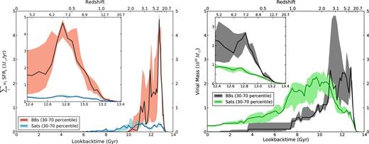
Left-hand panel: the star formations rates (M⊙ yr−1) of the fully disrupted building blocks (black line with red band) and the surviving satellites (blue line with light blue band) in haloes A–E, weighted by the mass of that galaxy at that time of star formation. At each time, the sum of the weights of the fully disrupted building blocks as well as those of the surviving satellites add up to one for each of these five Aquarius haloes (∑iwi = 1), after which the median is plotted (black and blue lines) as well as the 30–70 percentiles (red and light blue bands). The corresponding redshift is shown at the top axis. In the zoom-in panel, the SFRs in the first Gyr are shown. Adding those satellites that are stripped by at least two-thirds of their original stellar mass to the building blocks (to include also the main progenitors of spheroids C and D) did not significantly change this figure. Right-hand panel: the same mass-weighting is used to show the 30–50–70 percentiles of haloes A–E virial masses of building blocks as a function of lookback time (black line with grey band) and those of surviving satellites (green line with light green band). Again, the zoom-in panel shows the first Gyr of galaxy formation.
To shed some light on the origin of the difference in SFR between building blocks and surviving satellites, we show in Fig. 7 the virial mass versus SFR for all galaxies that still have their own dark matter halo at six different timesteps in the early universe. Galaxies that end up as building blocks are marked as yellow squares, whereas galaxies that survive as a satellite galaxy to the present day are visualized as blue circles. From this figure, it is clear that until ∼11.5 Gyr ago, the most massive galaxies are those that are building blocks at the present epoch. These building blocks are thought to be associated with high-density peaks that collapsed at higher redshifts, compared to the present-day surviving satellites that descended from more average density fluctuations in the early universe (Barkana & Loeb 2001; Diemand, Madau & Moore 2005). At early epochs, these satellites have lower virial masses than the building blocks, resulting in longer time-scales for merging with the central galaxy and lower SFRs. This same trend is shown in the right-hand panel of Fig. 6 where we apply the same mass weighting as we did to show the median SFR of the brightest objects at a particular lookback time, this time to show the median virial mass of the same objects (as well as the 30–70 percentiles again). The fact that the curves in the right-hand panel are decreasing after some time is due to tidal disruption of the haloes. Note that at the same time (∼11 Gyr ago), the SFR of the building blocks drops below that of the satellites (left-hand panel of Fig. 6) as their virial mass drop below that of the satellites (right-hand panel of Fig. 6).
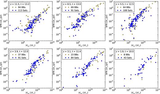
Virial mass versus SFR for the galaxies that become building blocks (yellow boxes) and the ones that survive as satellites (blue circles), at six different timesteps. The time and redshift labels are shown in the upper left corner of the panels. Also the total number of objects at that timestep is indicated in the legend of each panel.
5 COMPARISON OF BUILDING BLOCKS AND SURVIVING SATELLITES THROUGH THE STAR FORMATION TIMESPAN
5.1 Time-scales of growth
As already shown in the previous section, we find in our simulations that the average SFR in the surviving satellites is lower than in building blocks of the same mass (see Fig. 5), so it generally takes them a longer time to form their stars. This is visualized in more detail in Figs 8–11.
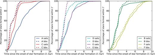
Percentage of stars in surviving satellites (solid lines) versus building blocks (dashed lines) that is formed since the onset of star formation. For spheroids A and C (left-hand panel), the difference between the two populations is very large already after ∼1 Gyr; for spheroids D and E (middle panel), the difference is largest after ∼2 Gyr; whereas for spheroids B and F (right-hand panel), the difference is negligible. All building blocks that form the stellar spheroid are included, also the stripped material from surviving satellites.
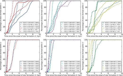
Percentage of stars formed since the onset of star formation in the three most massive surviving satellites that have lost less than 20 per cent of their stars (top three panels) and the three most massive building blocks that have been fully disrupted (bottom three panels). As in Fig. 8, spheroids A and C are visualized in the left-hand panels, spheroids D and E in the middle panels and spheroids B and F in the right-hand panels. Each colour indicates a separate spheroid, the same colour coding is used as in Fig. 8. The percentage of the total mass in satellites/building blocks that is contained in a particular satellite/building block is given in brackets in the legend of each panel. The most massive surviving satellites shown here (numbers 1) of spheroids B (indicated with the green solid line in the top right panel), D (the cyan solid line in the top middle panel) and E (magenta solid line in the top middle panel) lost, respectively, 6 per cent, 2 per cent and 2 per cent of their initial mass through tidal stripping, the other satellites did not lose any mass.
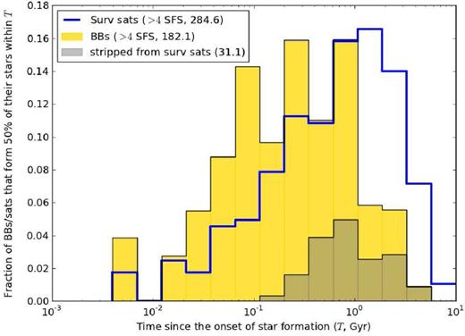
Fraction of building blocks (filled gold histogram) and surviving satellites (transparent histogram with thick blue edge) with more than four SFS that form 50 per cent of their stars within the time since the onset of star formation (T, Gyr), for the six Aquarius haloes combined. ‘Building blocks’ that are stars stripped from surviving satellites are divided among the two populations according to the mass fraction of the initial satellite mass. The dark shaded filled histogram shows how this material contributes to the building block distribution. The total number of building blocks and surviving satellites in these distributions are shown in brackets in the legend.
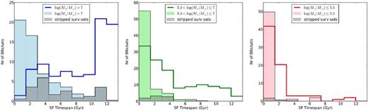
Number of building blocks (filled histograms) and surviving satellites (transparent histograms with thick edges) with more than four SFS per timespan it took to form all their stars (SF Timespan, binned in bins of 1.5 Gyr). The populations are split up into three different stellar mass regimes. High-stellar mass building blocks/satellites (M* > 107 M⊙) are shown with blue colours in the left-hand panel, intermediate-stellar mass building blocks/satellites (105.5 < M*/M⊙ ≤ 107) with green colours in the middle panel and low-stellar mass building blocks/satellites (M* ≤ 105.5 M⊙) with red colours on the right. With a dark shading, the material stripped from surviving satellites is indicated again.
The mass build-up of the accreted stellar spheroids (in percentage of the total accreted mass over time) since the beginning of star formation is shown for both building blocks and surviving satellites in Figs 8 and 9. For each galaxy, the moment at which the first stars in that galaxy begin to form is set as the zero time T. If a surviving satellite or building block experienced a merger with another galaxy, the star formation histories of the two galaxies are added together. The galaxy after the merger is therefore always considered to have started forming stars as early as the earliest of the two galaxies started to form stars. We do not examine the complete merger histories of building blocks and satellites here, but Deason, Wetzel & Garrison-Kimmel (2014b) estimated that ∼10 per cent of the dwarf galaxies with a stellar mass >106 M⊙ that are within the virial radius of the host experienced a major merger since z = 1.
Compared with the lookback time (used the previous sections in Figs 1, 2, 3 and 6), the onsets of star formation are shifted so that they all start at the same zero time, thus allowing us to address the enrichment histories of the building blocks and satellites on a similar internal time-scale. This is particularly relevant since several enrichment processes have longer delay time than others; e.g. SNe Type Ia originate from lower mass progenitors than SNe Type II and thus the former can only contribute significantly to enrich the galaxy after a certain time since the onset of star formation. The relative contributions of these SN types will have their imprint on the chemical abundances of the next generations of stars; whereas SNe Type II are producing lots of α-elements such as Mg, Ca and Ti, SNe Ia that are thought to be the main contributors for Fe for instance. The shifts that we applied, from the universal time to T, are no more than 0.1 Gyr for the most massive building blocks (of which we plotted the SFR in Fig. 2) and no more than 0.5 Gyr for the three most massive satellites of each spheroid.
We see that in spheroids A and C (leftmost panel of Fig. 8), ∼50 per cent of the stars in building blocks are formed within one Gyr, whereas only 10–30 per cent of the stars in the surviving satellites are formed during this timespan. For spheroids D and E (middle panel), the difference between the two percentages is the largest after approximately 2 Gyr, when ∼70–80 per cent of the stars in the building blocks were formed, compared to ∼40 per cent in the satellites. For spheroids B and F (right-hand panel), however, the difference between the build-up of the two populations of stars is much smaller.
In Fig. 9, we show the same growth rates for the surviving satellites (top panels) and the building blocks (bottom panels) as in Fig. 8, but now split out into contributions from three massive progenitors/surviving satellites in the population. As in Fig. 8, spheroids A and C, D and E and B and F are shown from left to right. The solid lines in the top panels and the dashed lines in the bottom panels correspond to the most massive satellites that have lost less than 20 per cent of their stars and most massive building blocks that have been fully disrupted, respectively, the second and third most massive galaxies are shown with other linestyles (see the legend). The contribution of that particular object to the total stellar mass in satellites or building blocks is given in between brackets in the legend of each panel. This gives an estimate of the weighting of that line with respect to the total build-up of satellites or building blocks over time (Fig. 8).
From Fig. 9, we learn that the spread in stellar mass build-up over time for massive satellites is larger than for massive building blocks. Comparing Figs 8 and 9, we see that the most massive surviving satellites (shown with solid lines in the top three panels of Fig. 9) resemble quite well the total build-up of the satellites in that spheroid over time (solid lines in Fig. 8). The same is true for the most massive building blocks of spheroids B and E, i.e. the dashed lines in the bottom panels of Fig. 9 match the dashed lines in Fig. 8 for these spheroids quite well. For spheroid A, on the other hand, the second most massive building block shown in Fig. 9 forms many more stars in a short period of time than the most massive one, thereby increasing the total percentage of stars formed early on. For the other spheroids (in particular, spheroid F), there is also a discrepancy between the dashed lines in the bottom panels of Fig. 9 and those in Fig. 8 because the most massive progenitor is not fully disrupted and therefore not included in Fig. 9.
Focusing now on the timespan during which the first 50 per cent of the stars in a building block/surviving satellite are formed, we show an overview of this distribution in Fig. 10. From this, it is once again clear that the building blocks form the first 50 per cent of their stars in a shorter time than the surviving satellites on average, as we expected from Figs 8 and 9. In Fig. 10, the time since the onset of star formation (T, Gyr) is binned in 15 equal-size bins on a logarithmic scale from 10−2.4 to 10 Gyr. We left out the building blocks/surviving satellites that had star formation in less than or equal to four snapshots again, which would otherwise pile-up in the lowest bin. The contribution from stripped surviving satellites is divided among the two populations according to the mass fraction. For example, the most massive progenitor of spheroid D is counted as 0.94 building block and 0.06 surviving satellite. With a dark shading in the building block histogram, we show that this material follows a different distribution than the total building block population and is more similar to that of the surviving satellites.
Finally, in Fig. 11, we split the total number of building blocks/surviving satellites up into three mass regimes, i.e. massive (>107 M⊙, in blue), intermediate mass (105.5 < M/M⊙ ≤ 107, in green) and low mass (≤105.5 M⊙, in red) shown from left to right, respectively. For the building blocks, indicated again with filled histograms, the fraction of stars in the lowest time bin relative to the total in that mass regime becomes larger if they are less massive, thus the chance that they formed their stars in a short timespan becomes larger with decreasing mass. However, the shape of the distribution is peaking at the shortest timespan in all three mass regimes for the building blocks. The opposite is true for the surviving satellites: the probability density function of the massive satellites peaks at large timespans, and the peak moves towards shorter timespans if the satellites become less massive, towards a distribution that is similar in shape to that of the building blocks for the lowest mass satellites. The ‘building blocks’ that were stripped from surviving satellites are indicated again with a dark shading, and as in Fig. 10, they are divided among the two populations according to the mass fraction of the initial satellite mass.
The three stellar mass bins chosen in Fig. 11 represent the various classes of dwarf satellite galaxies surrounding the Milky Way (as illustrated in comparison with Fig. 4). From the observed trends with stellar mass, we can conclude that the population of the faintest (also called ‘ultra-faint’) dwarfs show slightly more overlap in their star formation properties with the building blocks of similar mass than the brighter ‘classical’ dwarf galaxies.
5.2 Relation between iron abundance and SNe Type Ia delay time distribution
One key observable of our Milky Way system is that although its halo population is α-rich (Hawkins et al. 2014; Jackson-Jones et al. 2014), its (classical) satellites are predominantly α-poor, with an exception for their most metal-poor components (e.g. Shetrone et al. 1998, 2001, 2003; Tolstoy et al. 2003; Venn et al. 2004; Koch et al. 2008; Kirby et al. 2010; Starkenburg et al. 2013b; Frebel & Norris 2015; Jablonka et al. 2015). At metallicities of [Fe/H]∼−1, stars in the local halo have [α/Fe] ratios ([α/Fe] ∼ 0.2–0.4) that are approximately 0.2–0.6 dex higher than those in dwarf galaxies in the Local Group (see for a review, Tolstoy et al. 2009).
Several modelling efforts have already pointed out that indeed such a discrepancy could arise in a stellar halo built out of few early-accreted, massive main progenitor galaxies. These would have had high SFRs and have been enriched primarily by Type II SNe, whereas the surviving satellites had lower SFRs over a longer period of time, during which also Type Ia SNe contributed to their metal content, resulting in a lower [α/Fe] abundance (Robertson et al. 2005; Font et al. 2006a,b; Geisler et al. 2007). If Type Ia SNe start to contribute significantly only after a certain time-scale, this causes the [Fe/H] ratio to increase with respect to [α/H], leading to a ‘knee’ in the [Fe/H] versus [α/Fe] diagram. Support for such a scenario comes from the position of the observed knee in various galaxies; the α-element knee of the Sculptor dSph, for example, is estimated to be around [Fe/H]≈−1.8 (Tolstoy et al. 2009), whereas for the more massive Sagittarius, it takes place at [Fe/H]≈−1.3 (De Boer et al. 2014). This is consistent with our Fig. 11, where we see that the higher mass satellites have a higher SF efficiency, especially at earlier times.
As discussed before, our semi-analytic model does not include finite stellar lifetimes, but is based on an instantaneous recycling approximation, and therefore the relative contribution from Type Ia SNe and Type II SNe are not modelled directly. However, from the distribution of star formation timespans in the various building blocks and satellites as shown in Figs 8–11, we can still infer some information on the [α/Fe] ratios expected. For instance, by making the (very rough, but common) assumption that all spheroid stars formed after a certain time T, say 1 Gyr, are significantly enriched in iron from Type Ia SNe, and those before that time are α-rich, we can use Fig. 8 to predict that of the six Aquarius haloes, spheroids A and C have the most dominant high-α populations, spheroids B and F the least. De Lucia et al. (2014, 2015) have investigated the implementation of different delay time distributions for SN Ia explosions within a semi-analytical model that includes chemical evolution, but which is otherwise very similar to ours. They conclude that the Milky Way stellar disc metallicity distribution function is best represented for delay time distributions that are fairly broad, rather than strongly peaked at either short or intermediate delay times. In all these cases, the effective [O/Fe] yield (for a simple stellar population at fixed metallicity) is at a level ∼0.25 dex lower and most steeply dropping around a 1 Gyr time-scale, consistent with our simple assumption.
We see from Fig. 10 that 99 per cent of the building blocks and 92 per cent of the surviving satellites form the first 50 per cent of their stars in 3.3 Gyr. The observed discrepancy in [α/Fe] values between the stellar halo and the satellites of the Milky Way would therefore not be expected to show up in any of our modelled haloes, making 3.3 Gyr an upper limit on the delay time-scale for SNe Ia to become significantly abundant in the chemical enrichment process. Should on the other hand the relevant contribution delay time be as small as 6.5 × 10⁻² Gyr, then only 19 per cent of the building blocks would be α-rich, versus 10 per cent of the satellites. A difference that small would also be inconsistent with observations, making 6.5 × 10⁻² Gyr a lower limit on this time-scale.
We would like to note that although the exact distribution of type Ias as a function of time is highly uncertain (see e.g. Matteucci et al. 2009; Maoz, Mannucci & Nelemans 2014), many authors find that the delay time distribution has a power-law form, ∝ t−1, according to which ∼50 per cent of the Type Ia SNe occur within ∼1 Gyr. The time-scale T discussed here represents a cumulative result of all SNe Ia explosions on the galaxy enrichment, capable of moving from a regime of forming predominantly high-α stars to low-α stars, not the time-scale at which these stars start exploding. In the solar neighbourhood, the change of the [O/Fe] slope around [Fe/H] = −1 in the [O/Fe] versus [Fe/H] diagram is consistent with galactic chemical evolution models in which the overall delay time-scale for significant SNe Ia enrichment is ∼1 Gyr (eg. Matteucci & Recchi 2001). These time-scales could be different in regions with a different SFR, such as the bulge or the outer disc (eg. Pipino & Matteucci 2009).
The [α/Fe] distribution function of surviving satellites versus that of the inner halo was already modelled in detail by Font et al. (2006a), who also concluded that the bulk of the halo formed from massive satellites accreted early on. As noted by Font et al. (2006b) and Johnston et al. (2008), we see that in our models, the net efficiency of star formation – and in particular, the difference therein between the building blocks and satellites – show some variations between the modelled Milky Way-like systems. This means that largely independent of the assumptions made for the exact delay time distributions and/or Fe-enrichment mechanisms, we might expect to see different [α/Fe] distributions in various Milky Way-mass systems depending on their detailed formation histories. From an observational point of view, this is an exciting prospect offering us a different angle by which the history of a stellar halo can be unravelled. Currently, we do not have a clear picture on the [α/Fe] ratio in external Milky Way-like haloes (although Vargas et al. 2014 measured [α/Fe] abundances of four stars in the outer halo of the Andromeda Galaxy and found them α-enriched) but this will very likely change in the era of the European Extremely Large Telescopes (see e.g. Battaglia 2011).
6 CONCLUSION
In this paper, we have investigated the accreted stellar spheroids of Milky Way like galaxies with the Munich–Groningen semi-analytical model of galaxy formation, combined with the high-resolution Aquarius dark matter simulations. Typically, each of the accreted spheroids was built by only a few main progenitor galaxies and the majority of stars that end up in our Milky Way-like stellar spheroids is 10–13 Gyr old. In three of our six galaxies (C, D and F), a large fraction of the spheroid stars is stripped from satellites that are surviving to the present day. For spheroids C and D, these may be resembling the Sagittarius dwarf's contribution to the Milky Way halo. Spheroid F is atypical as a Milky Way analogue because it accreted ∼1010 M⊙ in stars over the last ∼3 Gyr.
We compared the properties of the building blocks of the Milky Way's stellar spheroid to those of the surviving satellites and found that in terms of the stellar mass–metallicity relation, the difference between the two populations is small, but that the former have significantly higher SFRs on average – they form comparable amounts of stars in a shorter time (see Figs 6 and 11). In particular, the more massive surviving satellites show a larger variety in stellar mass build-up over time than the massive building blocks (Fig. 9). On the other hand, the faintest surviving satellites build up mass in a similar fashion to building blocks with similar mass (right-hand panel of Fig. 11).
From these results, we expect the stellar spheroid to be more enriched in α-elements compared to Fe than the surviving satellites, as we observe in the Milky Way system. However, a quantitative analysis of the detailed chemical evolution will require a more sophisticated model and accurate descriptions of the delay time for SNe Type Ia. Furthermore, we are dealing with a stochastic process since we are comparing the spheroids of only six Milky Way-like galaxies, that have accreted components which are dominated by a few objects. This results in some of the Aquarius haloes having a better match with the Milky Way galaxy in terms of overall stellar mass and spheroid metallicity, while others have an accretion history that more closely matches that of the Milky Way. Also, we observe some scatter from system to system in our models of the time-scale of star formation in satellite galaxies and the time-scale of star formation in the main halo. A prediction of these models is therefore that not all Milky Way-mass systems will show [α/Fe] ratios similar to those in the Milky Way.
The authors are indebted to the Virgo Consortium, which was responsible for designing and running the halo simulations of the Aquarius Project and the L-Galaxies team for the development and maintenance of the semi-analytical code. In particular, we are grateful to Gabriella De Lucia and Yang-Shyang Li for the numerous contributions in the development of the code. Furthermore, we would like to thank the anonymous referee for valuable comments that helped to improve this paper. PvO thanks the Netherlands Research School for Astronomy (NOVA) for financial support. ES gratefully acknowledges funding by the Emmy Noether program from the Deutsche Forschungsgemeinschaft (DFG). AH acknowledges financial support from a VICI grant.
REFERENCES
