


The article ‘Formation and X-ray emission from hot bubbles in planetary nebulae – I. Hot bubble formation’ was published in 2014, MNRAS, 443, 3486 (hereafter Toalá & Arthur 2014). During revision of the follow-up paper (Part II. X-ray Emission, Toalá & Arthur 2016) we discovered an error in the energy update step of the thermal conduction routine in our numerical simulations. This caused extra energy to be added to the calculation and accelerated the expansion of the models with conduction. We also found that the size of the stellar wind injection region in our simulations plays an important role once the stellar wind mechanical luminosity drops off and the bubble starts to collapse. Our original calculations had a large (∼30 cells) wind injection region, which stalled the returning inner wind shock instead of letting it continue to collapse towards the star. Those simulations were then able to continue to late times and the stellar wind bubble expanded once more.
To remedy the first of these problems we completely rewrote the thermal conduction routine and subjected it to extensive testing. We ran tests on both the 1D spherical symmetric and 2D cylindrically symmetric versions of the code. We are now satisfied that our thermal conduction routine does not inject additional energy into the system and that we can account for all energy losses and gains (due to radiative cooling and photoionization, respectively). Thermal conduction is demonstrated not to affect the expansion rate of the stellar wind bubble but radiative cooling does.
The second problem was easily resolved by reducing the size of the stellar wind injection region (to 5 cells radius). Our new simulations give a more accurate representation of the hot bubble expansion around the time when the stellar wind mechanical luminosity drops off. Unfortunately, the timestep then becomes so small that none of the simulations advances much beyond this point and we do not get a re-expansion of the hot bubble. The majority of our hot bubbles do not reach a radius of 0.2 pc [as presented in Toalá & Arthur (2014)].
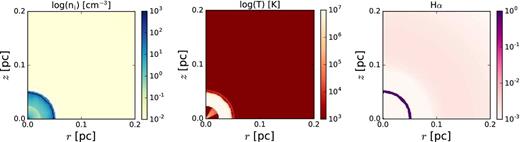
We present new versions of Figs 5–10, which show the number density of ions nI, the temperature and the Hα emissivity of the 1.5-0.597, 2.5-0.677 and 3.5-0.754 models for the cases with and without thermal conduction. The early-time evolution of the new simulations (not shown) is very similar to the old results, although the fine details of the instabilities vary since the stellar wind injection region is much smaller in the new calculations. For the 1.5-0.597 models, the new Figs 5 and 8 correspond to the time when the average hot bubble radius is 0.2 pc. For the 2.5-0.677 and 3.5-0.754 simulations, the new Figs 6, 7, 9 and 10 correspond to the time when the central star luminosity falls off and the calculation stalls.
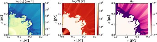
Total ionized number density (left-hand panel), temperature (middle panel) and normalized Hα volume emissivity (right-hand panel) for the PN formation for the 1.5-0.597 model 2D simulation without thermal conduction. The simulation corresponds to 7400 yr of post-AGB evolution for this CSPN, when the central star has an effective temperature and luminosity of log Teff = 5.0 and log L/L⊙ = 3.6.

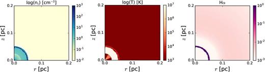
Same as Fig. 5 but for the case of 2.5-0.677 model without thermal conduction. The simulation corresponds to 2600 yr of post-AGB evolution for this CSPN, when the central star has an effective temperature and luminosity of log Teff = 5.29 and log L/L⊙ = 3.47.
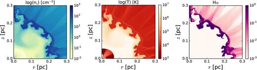
Same as Fig. 5 but for the case of 3.5-0.754 model without thermal conduction. This set of panels corresponds to 780 yr of post-AGB evolution for this CSPN, when the central star has an effective temperature and luminosity of log Teff = 5.2 and log L/L⊙ = 4.08.
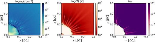
Same as Fig. 5 but for the 1.5-0.597 model with thermal conduction after 7400 yr of post-AGB evolution for this CSPN, when the central star has an effective temperature and luminosity of log Teff = 5.0 and log L/L⊙ = 3.6.
Same as Fig. 5 but for the case of 2.5-0.677 model with thermal conduction after 2600 yrs of post-AGB evolution for this CSPN, when the central star has an effective temperature and luminosity of log Teff = 5.29 and log L/L⊙ = 3.47.
Same as Fig. 5 but for the case of 3.5-0.754 model with thermal conduction after 780 yr of post-AGB evolution for this CSPN, when the central star has an effective temperature and luminosity of log Teff = 5.2 and log L/L⊙ = 4.08.
We also present here a revised version of Fig. 11, which compares 2D results to 1D simulations at the same resolution with the same physical processes for the 1.5-0.597, 2.5-0.677 and 3.5-0.754 models. An essential difference is the evolution time at which the latter two models are shown, which corresponds to when the calculations stall, rather than the much later times shown in the original paper. From the new Fig. 11 we note that the differences between the 1D and angle-averaged 2D simulations in the 1.5-0.597, 2.5-0.677 models is due to the instabilities that arise in the 2D cases. The instabilities enable hot gas to penetrate through the corrugated swept-up shell to larger radii than are seen in the 1D case. For the 3.5-0.754 models, there is a large discrepancy between the 1D and 2D models with regard to the positions of the shocks and contact discontinuities. This is due to overcooling at the contact discontinuity at very early times in the 1D calculations due to the low numerical resolution used in these calculations.
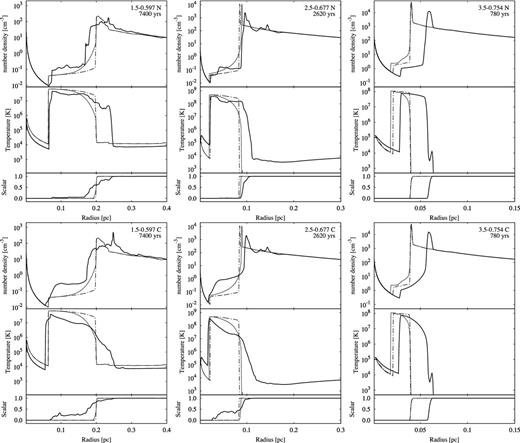
Comparison of 2D results with 1D results. Top row – 2D results without thermal conduction. Bottom row – 2D results with thermal conduction. In each plot, the upper panel shows the total number density and the centre panel shows the temperature. The lower panel shows the value of a passive advected scalar. The thick solid line is the 2D simulation as a function of radius averaged over all angles from the stellar position. The thin solid line is the 1D result with thermal conduction and the broken line is the 1D result without thermal conduction, both at the same evolution time as the 2D result.
The mass in the hot bubbles in the new simulations including thermal conduction does not grow as fast as in the old simulations because the expansion rates of the bubbles are now lower. Fig. 12 shows the hot bubble mass as a function of time for the new 1.5-0.597 and 2.0-0.633 simulations. The models with conduction have higher hot bubble masses due to thermal evaporation of dense shell material in both 2D and 1D simulations. For the models without conduction, the 1D simulations have hot bubble masses on average less than or equal to the injected fast wind material.
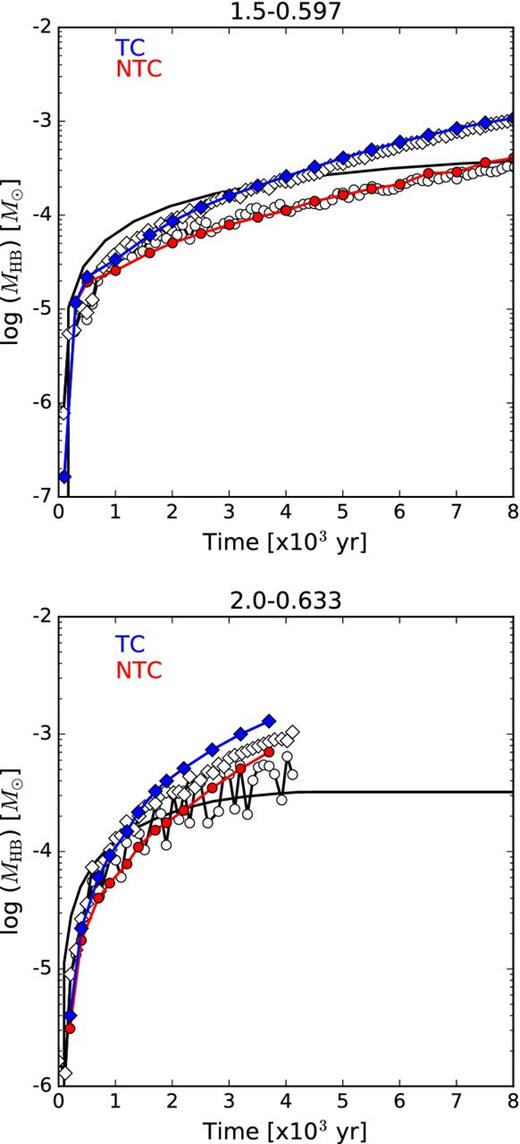
The hot bubble mass as a function of time for the 1.5-0.597 and 2.0-0.633 models. The solid lines without symbols represent the amount of mass injected by the fast wind. The lines with circles (red) represent the total mass of the hot bubble without thermal conduction, while the diamonds (blue) represent the model with thermal conduction. Open symbols represent the corresponding 1D simulation results.
The radial velocity of the photoionized shell (the W-shell) also changes in the new simulations. This is shown in Fig. 13, where we see closer agreement between the shell velocities for models with and without conduction than was obtained with the old calculations. On the other hand, the shell velocities for the 2D simulations are higher than those obtained previously. This is because the stellar wind injection region is now smaller and there are differences in the formation and evolution of the instabilities. The density-weighted mean radial velocity of the photoionized gas in the W-shell is computed over all cells having ionized number density above 200 cm−3, radial velocity below 60 km s−1 and scalar value between 0.7 and 1.0. The old calculations produced more pronounced corrugations in the shell and lower mean radial velocities. The new simulations form shells that are less fragmented and have a more uniform expansion velocity.
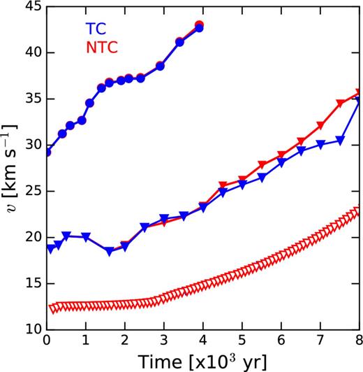
W-shell velocity as a function of time for the 1.5-0.597 (triangles) and 2.0-0.633 (circles) models. Models including thermal conduction are represented with filled (red) markers. The corresponding 1D results for the 1.5-0.597 model are shown with dotted lines and open triangles.
The main conclusions of Toalá & Arthur (2014) are unchanged, although the differences between models with and without thermal conduction are less pronounced. However, our claim that hot bubbles with thermal conduction are self-sealing cannot be confirmed with the new simulations because the calculations stall before this occurs.
Acknowledgments
We acknowledge the comments of the referee of Toalá & Arthur (2016), Dr. Detlef Schönberner, whose suggestions led to the revision of our numerical code.
