


Abstract
Using the Sloan Digital Sky Survey, we adopt the specific star formation rate (sSFR)–Σ*,1kpc diagram as a diagnostic tool to understand quenching in different environments. sSFR is the specific star formation rate and Σ*,1kpc is the stellar surface density in the inner kpc. Although both the host halo mass and group-centric distance affect the satellite population, we find that these can be characterized by a single number, the quenched fraction, such that key features of the sSFR–Σ*,1kpc diagram vary smoothly with this proxy for the ‘environment’. Particularly, the sSFR of star-forming galaxies decreases smoothly with this quenched fraction, the sSFR of satellites being 0.1 dex lower than in the field. Furthermore, Σ*,1kpc of the transition galaxies (i.e. the ‘green valley’ or GV) decreases smoothly with the environment by as much as 0.2 dex for M* = 109.75–10 from the field, and decreasing for satellites in larger haloes and at smaller radial distances within same-mass haloes. We interpret this shift as indicating the relative importance of today's field quenching track versus the cluster quenching track. These environmental effects in the sSFR–Σ*,1kpc diagram are most significant in our lowest mass range (9.75 < log M*/M⊙ < 10). One feature that is shared between all environments is that at a given M*, quenched galaxies have about 0.2–0.3 dex higher Σ*,1kpc than the star-forming population. These results indicate that either Σ*,1kpc increases (subsequent to satellite quenching), or Σ*,1kpc for individual galaxies remains unchanged, but the original M* or the time of quenching is significantly different from those now in the GV.
1 INTRODUCTION
Identifying the physical mechanisms that cause and sustain the cessation of star formation in galaxies has been a persistent problem in galaxy evolution research. Studies of large surveys over the last decade have made significant progress towards understanding this problem. In particular, it is now firmly established that the galaxy population obeys three broad correlations between morphology, environment and quenching: (1) quenched galaxies tend to have early-type morphology or dense structure, (2) quenched galaxies tend to live in dense or massive halo environments and (3) galaxies with early-type morphologies are found in these dense environments.
1.1 Quenching and morphology/structure
Ever since Hubble classified the galaxies (Hubble 1926), it has been known that the galaxy population can be roughly divided into star-forming (SF) discs and quenched spheroids. Early-type morphologies or high stellar density strongly correlate with being quenched in the local universe (eg. Strateva et al. 2001; Blanton et al. 2003; Kauffmann et al. 2003; Bell 2008; van Dokkum et al. 2011; Fang et al. 2013; Bluck et al. 2014; Omand, Balogh & Poggianti 2014; Schawinski et al. 2014) and at high-z (Wuyts et al. 2011; Bell et al. 2012; Cheung et al. 2012; Szomoru, Franx & van Dokkum 2012; Wuyts et al. 2012; Barro et al. 2013; Lang et al. 2014; Tacchella et al. 2015).
One manifestation of this correlation between morphology and quenching is that the mass profiles of quenched and SF galaxies differ within the inner 1 kpc such that quenched galaxies are denser in this inner region (Fang et al. 2013). (This is illustrated in Fig. 1 which is a schematic diagram of specific star formation rate (sSFR) versus the stellar density within 1 kpc Σ*,1kpc. The quenched population, marked ‘Q’, has at high Σ*,1kpc relative to the star–forming population, marked ‘SF’.) At any time, this central stellar density grows along with stellar mass while on the galaxy main sequence (Hopkins et al. 2009; Feldmann et al. 2010; van Dokkum et al. 2015). The high inner densities seen in quenched galaxies today were already in place by z ∼ 2 (Patel et al. 2013; Barro et al. 2015; Tacchella et al. 2015), which may suggest that if there is a connection between quenching and high inner density, it likely occurs at high-z.
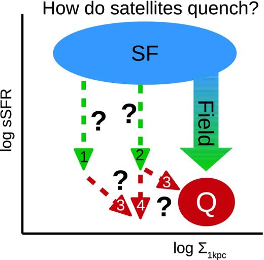
Schematic diagram illustrating quenching paths in sSFR–Σ*,1kpc space at constant stellar mass. The region marked ‘SF’ refers to the ‘star-forming’ population and the region marked ‘Q’ refers to the ‘quenched’ population. The possible satellite quenching paths are the subject of this study. The numbered arrows are discussed in Section 1.4.
Several ideas have been proposed to explain this observed link between morphology and quenching. Major dissipative mergers, for instance, have been demonstrated in simulations to build a central spheroid component through violent relaxation of pre-merger stars (Toomre & Toomre 1972; Mihos & Hernquist 1994; Hopkins et al. 2009). The dissipative inflow of gas triggers a central starburst that, along with contributing to the bulge, also quenches a galaxy through fast consumption and/or winds. In simulations, the same inflow can accompany disc instabilities (Friedli & Benz 1995; Immeli et al. 2004; Bournaud et al. 2011) which are observed in local galaxies (Courteau, de Jong & Broeils 1996; Carollo, Stiavelli & Mack 1998; Carollo et al. 2001, 2007; MacArthur, Courteau & Holtzman 2003; see also the review by Kormendy & Kennicutt 2004). Violent disc instabilities are predicted in simulations to be especially relevant at high-z (Noguchi 1999; Bournaud, Elmegreen & Elmegreen 2007; Dekel, Sari & Ceverino 2009; Dekel & Burkert 2014; Mandelker et al. 2014). Instabilities can also be triggered by mergers (Barnes & Hernquist 1991; Mihos & Hernquist 1996; Hopkins et al. 2006; Zolotov et al. 2015) and counter-rotating streams (Danovich et al. 2015). A candidate merger sequence has been identified at z ∼ 0 observations extending all the way from disturbed starbursts followed by fading, active galactic nuclei (AGN) turn-on and eventual quiescence (Yesuf et al. 2014; see also Ellison et al. 2011).
While there is a structural correlation with quenching, its causality arrow is not clear. It may be the effect of quenching that is unrelated to morphology (Lilly & Carollo 2016). It has also been argued and shown that a spheroid can and sometimes does regrow a SF disc (e.g. Brennan et al. 2015; Graham, Dullo & Savorgnan 2015) unless accretion is prevented, for example, in a hot massive halo (Gabor & Davé 2015; Woo et al. 2015; Zolotov et al. 2015) and/or by AGN (Dekel & Birnboim 2006; Kormendy & Ho 2013 and references therein). In addition, a significant number (25–65 per cent) of quenched galaxies appear to have (early-type) discs, especially at high-z (Stockton, Canalizo & Maihara 2004; McGrath et al. 2008; van Dokkum et al. 2008; van den Bergh 2009; Bundy et al. 2010; Oesch et al. 2010; van der Wel et al. 2011; Bruce et al. 2012, 2014; Salim et al. 2012), and also a number of bulges appear to be blue (e.g. Carollo et al. 2007).
1.2 Quenching and the halo environment
The quenched fraction for central galaxies (those that are in the centres of their halo potential wells) correlates with various measures of the halo environment, including the halo mass Mh (Woo et al. 2013; Gabor & Davé 2015; Woo et al. 2015; Zu & Mandelbaum 2016). This is often attributed to virial shock heating of infalling gas in haloes more massive than Mcrit ∼ 1012 M⊙ (Croton et al. 2006; Dekel & Birnboim 2006). Below this critical mass, accretion is cold and conducive to star formation, while above it, infalling gas reaches the sound speed and a stable shock forms, heating the gas (Rees & Ostriker 1977; Birnboim & Dekel 2003; Kereš et al. 2005; Dekel & Birnboim 2006). For a population of haloes, this is manifested as a mass range extending over one or two decades around Mcrit where there is a decrease in the cold accretion as a function of halo mass (Mh) (Ocvirk, Pichon & Teyssier 2008; Kereš et al. 2009; van de Voort et al. 2011).
Since the effects of this so-called halo quenching are expected to increase with the mass of the halo rather than galaxy stellar mass, they are seen most dramatically in the satellite population since their host haloes can be much more massive than those of field galaxies at the same stellar mass. These effects are seen as ‘environment’ quenching in which the galaxy population is more likely to be red or have low sSFR in dense environments (Hogg et al. 2003; Balogh et al. 2004; Kauffmann et al. 2004; Blanton et al. 2005b; Baldry et al. 2006; Bundy et al. 2006; Cooper et al. 2008; Bamford et al. 2009; Patel et al. 2009; Skibba & Sheth 2009; Wilman, Zibetti & Budavári 2010; Haas, Schaye & Jeeson-Daniel 2012; Quadri et al. 2012; Wetzel, Tinker & Conroy 2012; Hartley et al. 2013; Knobel et al. 2015; Carollo et al. 2016) and in massive haloes (Woo et al. 2013, 2015; Bluck et al. 2016).
Peng et al. (2010) argued that this environmental quenching is separable from the quenching that happens in the field (they call this ‘mass quenching’), but others have argued that halo quenching can affect both centrals and satellites (Gabor & Davé 2015; Woo et al. 2015; Zu & Mandelbaum 2016). Indeed, the question has been raised as to whether the apparent separability between quenching of centrals and satellites is actually a single phenomenon that masquerades as two separable processes due to the lack of dependence on halo mass of the mass function of the satellite population (Knobel et al. 2015; Carollo et al. 2016), or if quenching is merely a function of halo age (Hearin & Watson 2013). It remains an open question whether satellites experience additional quenching mechanisms than field galaxies, or merely more of the same physics that also quenches field galaxies.
1.3 Morphology/structure and the halo environment
The morphology of galaxies is also correlated with dense environments (Holmberg 1940; Dressler 1980). There is evidence that this so-called morphology–density relation is not due to environmentally-driven morphological change, but only to the increased quenched fraction in dense environments. For example, the early-type fraction of satellites, determined by visual classification, does not rise as steeply with decreasing group-centric distance as the quenched fraction of satellites (Bamford et al. 2009), and the early-type fraction of quenched satellites determined by a combination of parametric and non-parametric fitting) does not vary at all (Carollo et al. 2016) with distance. These authors use these observations to argue that the morphology–density relation is driven by the increase of the red fraction in dense environments rather than a real increase of early-type morphology in dense environments.
In fact, if there are two separate quenching channels for satellites as in Peng et al. (2010), Carollo et al. (2016) argue that both channels must have the same effect (either no or some effect) on the morphologies of satellites. If they are the same effect, then it is possible that a single mechanism governs the quenching of galaxies, the same mechanism that operates in the field (which is correlated with morphology/structure), and is simply more advanced in clusters. This idea has not yet been studied in detail.
1.4 Goals of this paper
In this paper, we aim to study the interplay of the above three correlations for satellite galaxies in order to clarify the role of the halo environment versus the role of morphology/structure-dependent quenching in governing their evolution. The diagnostic we will use is the diagram of the sSFR versus the stellar surface mass density within 1 kpc (Σ*,1kpc). The distribution of galaxies in this parameter space has been used for understanding structural change during quenching for centrals and their quenching track (labelled ‘Field’ in Fig. 1 – see Barro et al. 2013; Fang et al. 2013; Tacchella et al. 2015). This diagram has not yet been compared between environments.
Do satellites in different environments populate different regions of this diagram? Such a comparison will aid in understanding simultaneously how star formation activity and galaxy structure evolve for satellites and how this evolution differs from that of isolated galaxies. The various satellite quenching mechanisms proposed in the literature – ram pressure stripping, starvation, harassment – are expected to act on satellites regardless of their Σ*,1kpc. If such mechanisms are important in satellite evolution, their quenching track in sSFR–Σ*,1kpc space should resemble something like the arrow labelled ‘2’ in Fig. 1, i.e. in a different location than that of the field. In particular, if galaxies with low Σ*,1kpc tend to have more loosely bound gas, ram pressure stripping, in particular, may preferentially affect galaxies with low Σ*,1kpc, resulting in a quenching track more like arrow ‘1’ in Fig. 1. Some of these mechanisms may cause an increase in Σ*,1kpc via some triggered star formation during or after quenching (arrows ‘3’), or nothing more may happen to the satellites (arrow ‘4’). This paper attempts to detect any of these effects.
Even if satellites begin to quench independently of their Σ*,1kpc, their subsequent evolution in sSFR–Σ*,1kpc and even M* may not be simple to predict. Do satellite quenching mechanisms eventually change Σ*,1kpc or M*? The position of the quenched satellite population in this diagram relative to the position of transitioning satellites will shed light on these issues.
Note that the above correlations in the literature between morphology, environment and quenching were discovered using simply the quenched fraction. However, higher order information can be gained about the transition process as sSFR declines by studying the entire distribution of sSFR rather than just the quenched fraction (as emphasized by Woo et al. 2015). This kind of study is required for answering the questions posed here.
The literature is replete with many different measures of ‘structure’ and ‘morphology’. However, since they all strongly correlate with each other, the above correlations are likely to be true in broad strokes, regardless of which measure is used. In this paper, we adopt Σ*,1kpc (introduced by Cheung et al. 2012 and Fang et al. 2013) as our fiducial measure of structure for a number of reasons.
Despite some uncertainties in its measurement (such as the effect of the point spread function, PSF), it does not depend on galaxy radius, which is usually light-based in current catalogues (unlike, for example, the density within the effective light radius, Σe.)
It is measured directly from the data and not a fit to a model profile, which can be plagued by degeneracies and result in large systematic residuals.
It refers to the innermost part of a galaxy, which is arguably less affected by stripping.
The galaxy population seems to obey the same Σ*,1kpc–M* relation at low- and high-z (Tacchella et al. 2015, 2016 – or with only slight variation Barro et al. 2015), suggesting that Σ*,1kpc is a stable quantity that, on the whole, either stays constant with time or increases with time (as stellar mass increases). For individual galaxies, it is difficult to imagine how it could decrease.
Clearly, 1 kpc means very different things for galaxies of very different sizes (and thus masses). For this reason, we also confirmed that the same analysis using the bulge mass (Mendel et al. 2014) the Sérsic (1968) index n (Simard et al. 2011) instead of Σ*,1kpc produced similar results. This is, after all, not unexpected given the strong correlations between different measures of ‘morphology’ and ‘structure’.
Section 2 describes our selection and quantities used from the Sloan Digital Sky Survey (SDSS). Section 3 presents our findings regarding the distribution of satellites in the sSFR–structure plane compared to the field and as a function of the halo environment. Section 4 discusses possible implications of our results on the nature of satellite quenching.
This analysis assumes concordance cosmology: | $H_{\rm o} = 70\,{\rm km\,s^{-1} Mpc^{-1}}, \Omega _{\rm M} = 0.3, \Omega _\Lambda =0.7$ |. Our halo mass estimates also assume σ8 = 0.9, Ωb = 0.04.
2 DATA
2.1 The sample
The SDSS (York et al. 2000; Gunn et al. 2006) sample used here is from Data Release 7 (DR7; Abazajian et al. 2009). This sample contains 53 603 galaxies after matching all catalogues and applying all cuts as described below.
We limited the redshift range to 0.03 < z < 0.07 (in order to minimize seeing effects). Applying the K-correction utilities of Blanton & Roweis (2007) (v4_2) on ugriz photometry (‘petro’ values – Gunn et al. 1998; Doi et al. 2010), using redshifts from the New York University Value-Added Catalog (NYU-VAGC) DR7 catalogue (Blanton et al. 2005a; Adelman-McCarthy et al. 2008; Padmanabhan et al. 2008) and the r-band limit (17.77) of the spectroscopic survey, we calculate Vmax. Each galaxy is weighted by its 1/Vmax multiplied by the inverse of its spectroscopic completeness (also from the NYU-VAGC) in order to compute all quoted galaxy fractions and volume densities.
The NYU-VAGC contains 2506 754 objects, of which 153 662 lie within our chosen redshift range and are primary spectroscopic targets, 140 758 also have r-band magnitudes <17.77, and 137 756 of which kcorrect-produced finite Vmax. This sample was matched with other catalogues as described below.
2.2 Galaxy central density
Throughout the analysis, we make use of the stellar surface density within the inner kiloparsec Σ*,1kpc in order to probe quenching mechanisms which result in centrally concentrated galaxies. This is computed in the following way. Using the SDSS DR7 Catalogue Archive Server, we retrieved surface brightness profiles in the ugriz bandpasses and corrected them for galactic extinction using the extinction tags in the SpecPhoto table. The flux within each radial bin in all five bands is used as input into the K-correction utilities of Blanton & Roweis (2007) (v4_2) to compute the stellar mass profile. These bins are summed to produce the cumulative mass profile. Interpolating between the radial bins, we estimated the total mass and surface density within 1 kpc. (We confirmed that the largest radial bin for our final sample is greater than 1 kpc, and that their smallest radial bin is smaller than 1 kpc; i.e. it was not necessary to extrapolate to 1 kpc for any of our sample.)
This computation does not account for contamination from near neighbours or from effects of atmospheric seeing. However, Woo et al. (2015) showed that neither of these are important if the sample is selected such that the PSF full width at half-maximum (of a double Gaussian fit, i.e. the psfwidth in the r-band) is <2 kpc.
Out of 859 281 galaxies with profiles retrieved from CasJobs with z < 0.3, 142 852 make the redshift cut. We further selected 142 363 objects which are spectroscopically classified as galaxies (SpecClass = 2 from CasJobs), 135 300 of which also make the PSF cut.
We also cut the sample to exclude those that are highly inclined. Our cut of b/a > 0.5 leaves a sample of 97 603. Since inclined galaxies can only be discs (and not spheroids), this cut preferentially removes slightly less massive galaxies. These also tend to be green (mid-range g − r colour) since their inclination reddens a presumably SF galaxy. Since these are discs, they also tend to have lower Σ*,1kpc. Matching with the NYU-VAGC (after the above cuts) then produces 90 681 objects.
2.3 Stellar masses and star formation rates
Stellar mass and star formation rate (SFR) estimates are provided online by Brinchmann et al.1. These are derived through the fitting of spectral features in the spectral energy distribution (SED). The formal 1σ errors (from the 95 per cent confidence intervals of the probability density distribution) are typically ≲0.05 dex.
SFR estimates are an updated version of those derived in Brinchmann et al. (2004). The Kroupa (2001) initial mass function is used to calibrate these SFR estimates. Following the method of Brinchmann et al. (2004), these estimates combine measurements from inside and outside the fibre. Inside the fibre, H α and H β lines are used to compute SFR for SF galaxies. For galaxies with weak lines or showing evidence for AGN, SFR is estimated from an empirical relation between the D4000 break and H α and H β lines observed in SF galaxies. Outside the fibre, Brinchmann et al. fit SEDs to the observed photometry. The means of the probability density distributions of the SFRs inside and outside the fibre were added resulting in an estimate of total SFR.
Brinchmann (private communication) estimates the typical error of these SFRs to be about 0.4 dex for SF galaxies. For quenched galaxies, the errors are 0.7 dex or more, and these SFRs can be considered to be upper limits rather than measurements.
This catalogue contains 927 552, of which 163 686 pass our redshift cut. In addition, we limit our sample to those with M* > 109.75 M⊙ (102 998) and those for which the mode and mean of the probability density distribution of the SFR differed by no more than a factor of 20 (removing two galaxies). Applying the previous cuts reduces the sample to 60 621.
This study refers to ‘star-forming’ (SF) galaxies, those in the ‘green valley’ (GV) and those that are ‘quenched’ (Q). Since the main environmental effects in sSFR–Σ*,1kpc distribution are visible to the eye, they do not depend on any formal definition of these three populations, so we often refer to them qualitatively. In order to confirm our qualitative assessments from the sSFR–Σ*,1kpc diagrams, we investigate these three populations individually, and in these cases, we use the formal definition that is shown in Fig. 2. The lines were determined by eye and are defined as log sSFR(yr−1) = 0.2–0.92(log M*/M⊙ − 10) ± 0.2. Our results are not sensitive to reasonable variations in the slopes and zero-points of these lines.

2.4 The group catalogue and halo masses
Yang et al. (2012) constructed a group catalogue and estimated group halo masses for the SDSS DR7 sample based on the analysis of Yang et al. (2007). We use this catalogue with a slight modification as described in Woo et al. (2015) and which we briefly describe here.
Yang et al. (2007) applied a group finder that estimates the number density contrast of dark matter particles based on the centres, sizes and velocity dispersion of group members, assuming a spherical NFW profile (Navarro, Frenk & White 1997). Testing this group finder on a mock catalogue constructed from the conditional luminosity function model (see Yang et al. 2004), they found that their algorithm successfully selected more than 90 per cent of true haloes more massive than 1012 M⊙.
Once the group catalogue was constructed, Yang et al. (2007) estimated halo masses by rank-ordering the groups by group stellar mass and assigning halo masses according to a halo mass function. Comparing these halo masses with groups found in a mock catalogue, they find an rms scatter of about 0.3 dex.
The stellar masses used by Yang et al. (2007, 2012) are computed using the relations given by Bell et al. (2003), which can underestimate M* for dusty, SF galaxies. Thus, using the group catalogue of Yang et al. (2012), we recompute group masses using the stellar masses described in Section 2.3, which are estimated via SED fitting that incorporates dust. We applied the same correction for missing members as in Yang et al. (2007), and used the same technique for identifying the groups that are complete to certain redshifts. (Refer to their paper for details.) We used the Tinker et al. (2008) mass function using the Eisenstein & Hu (1998) transfer function to assign halo masses to the rank-ordered group masses. Our modifications to their method produce estimates for halo mass that are consistent with their estimates above Mh = 1012.6 M⊙. In the range of 12 < log Mh/M⊙ < 12.6, our estimates are, on average, 0.03–0.05 dex higher than theirs, which is expected given that dusty star-formers are found in this range. This catalogue from Yang et al. (2012) contains 633 310 galaxies, of which 587 575 match the stellar mass catalogue in Section 2.3.
This study compares galaxies which are satellites in groups with field galaxies. Of the 587 575 galaxies with modified Mh, 462 067 are the most massive member of their group. 415 750 of these are in groups of only one member, and these we call the ‘field’. Satellites are defined in the same way as in Woo et al. (2015) and the definition of the dynamical state of the group is taken from Carollo et al. (2013b). In particular, groups (with more than one member: 46 317) are assumed to be relaxed if the most massive member is also the nearest to the mass-weighted centre of the group (true of 37 921 groups; Cibinel et al. 2013; Carollo et al. 2013b). Otherwise, the group is potentially unrelaxed (8396). The first criterion for a satellite is that it must be a member of a relaxed group, and not be the most massive member (a total of 63 757 satellites). Secondly, if it is in potentially unrelaxed groups, a satellite must rank as third massive in the group or lower (adding 53 373 satellites). The idea behind the second criterion is that the group halo is most likely associated with the two most massive members. However, if we restricted our sample only to the first criterion, our results, though much noisier, would remain qualitatively unchanged. Table 1 summarizes how the group catalogue is divided into these categories.
Breakdown of the group catalogue.
| Original catalogue: | 633 310 | ||||
|---|---|---|---|---|---|
| after matching Section 2.3: | 587 575 | ||||
| Centrals: 462 067 | Satellites: 125 508 | ||||
| Field: | Group: | Relaxed: | Unrelaxed: | ||
| 415 750 | 46 317 | 63 757 | 61 751 | ||
| Relaxed: | Unrelaxed: | Rank = 2: | Rank > 2: | ||
| 37 921 | 8396 | 8378 | 53 373 | ||
Removing the most massive two galaxies of potentially unrelaxed groups clearly removes galaxies that are more massive than the general population. However, since our analysis compares satellites and the field at the same mass, this will not change our overall results.
Applying the previous cuts (in redshift, mass, etc), the field sample size reduces to 35 876, while the satellites sample reduces to 17 727.
We define the relative group-centric distance D of satellites as the ratio of the projected distance Rproj of each satellite to the mass-weighted group centre and the virial radius Rvir = 120(Mh/1011 M⊙)1/3kpc (e.g. Dekel & Birnboim 2006), i.e. D = Rproj/Rvir.
2.5 Mass completeness
We have used the above sample of 53 603 for the majority of our analysis, in particular, the sSFR–Σ*,1kpc diagrams. One part of our analysis also involves the quenched fraction which will be biased low due to lower completeness for red galaxies. Therefore, in the analysis that compares the quenched fraction between mass bins (i.e. Fig. 9), we used more stringent redshift cuts that result in a complete sample for red galaxies. These cuts are shown in Fig. 3. The resulting samples are 28 894 in the field and 14 820 satellites.

3 RESULTS
3.1 Structural properties of satellites and isolated galaxies
In order to understand the effect of the halo environment on structural/morphological properties, we compare these properties between satellite and field galaxies. While we compare these populations in the same M* bins, they lie in very different haloes. An analysis of the effect of the halo environment will follow in the next subsection.
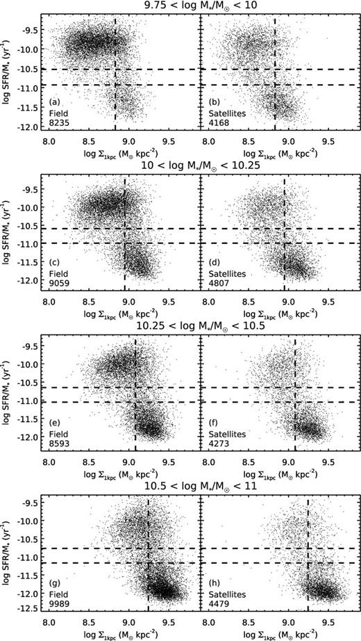
In Fig. 4, we show the distribution of sSFR (SFR/M*) and Σ*,1kpc for field (left-hand panels) and satellite galaxies (right-hand panels) in four bins of M* from top to bottom. The contours represent the logarithmic number density of the population in each panel (weighted by volume and smoothed – the raw points are shown in the Appendix in Fig. A1.) The contours in each panel clearly show the well-known bimodality in star formation between SF galaxies with high sSFR and quenched (Q) galaxies at low sSFR, bridged by a population of intermediate sSFR often called the GV. (We formally define these SF categories in Fig. 2. These divisions roughly correspond to the two horizontal lines in Fig. 4.) Fig. 4 shows that for both satellites and the field, in order to be quenched, galaxies need to have relatively high Σ*,1kpc for their mass bin (by 0.2–0.3 dex), as noted by Cheung et al. (2012) and Fang et al. (2013), as well as other authors using different measures of structure/morphology (see Section 1). In other words, there are no quenched galaxies with low Σ*,1kpc in a given mass bin.
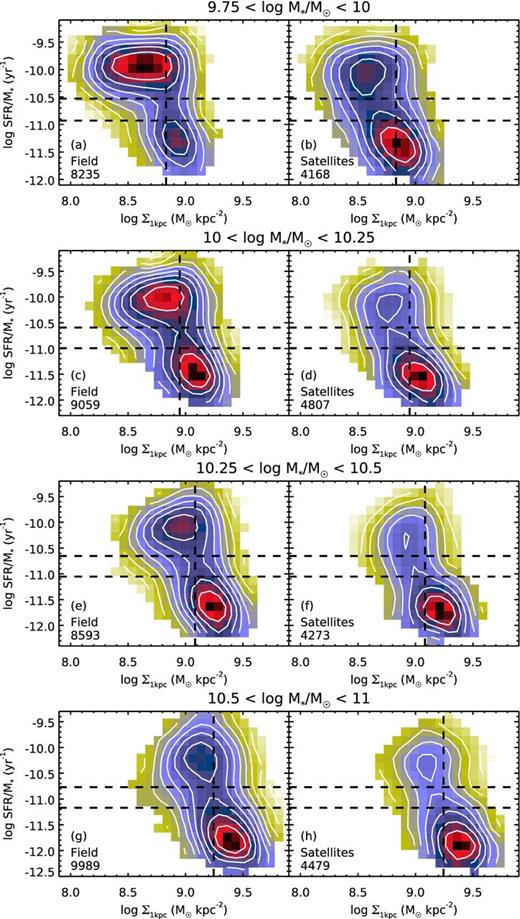
sSFR versus Σ*,1kpc comparing the field to satellites in four M* bins. The GV, as defined in Fig. 2, lies roughly between the two horizontal lines. For reference, the vertical line marks the median GV of the field. The contours represent the logarithmic number density in each panel and are separated by 0.2 dex. The colour scale is normalized such that dark red represents the highest number density in the panel. The sample size is indicated in the bottom left. Satellites have a higher proportion of quenched galaxies than the field at all masses. The GV bridge connecting the SF and Q populations lies at lower Σ*,1kpc for satellites than for the field (by ∼0.2 dex for the lowest mass bin). Quenched galaxies have higher Σ*,1kpc than SF galaxies by about 0.2–0.3 dex whether in the field or as satellites. These effects are strongest for the lowest masses and decrease in significance for the most massive galaxies.
But despite this overall similarity, Fig. 4 also shows that satellites occupy somewhat different regions of the sSFR–Σ*,1kpc plane than field galaxies, especially when considering the lowest mass bin (top two panels). Apart from the relative number of quenched satellites being higher than the quenched field galaxies in all mass bins (as found in many studies – see Section 1), there are also some notable differences.
Relative to the field galaxies, the GV ‘bridge’ between the two populations of the sSFR bimodality is shifted towards lower Σ*,1kpc for satellites. That is, this bridge lies at high Σ*,1kpc for the field galaxies, and at more mid-range values of Σ*,1kpc for satellites. The effect is a shift in Σ*,1kpc of ∼0.2 dex for the lowest mass bin and less than 0.1 dex for the highest. (For reference, the vertical lines in Fig. 4 show the median Σ*,1kpc of the field GV in each mass bin.)
Perhaps related to this, the lowest Σ*,1kpc edge of the Q population for satellites appears stretched towards lower Σ*,1kpc relative to the Q field.
The centroids of both the SF and Q populations are slightly lower in sSFR for satellites (by about 0.1 dex – see Fig. 6 which is described below; it is also seen in the peaks of the one-dimensional sSFR distribution – see Fig. 5).
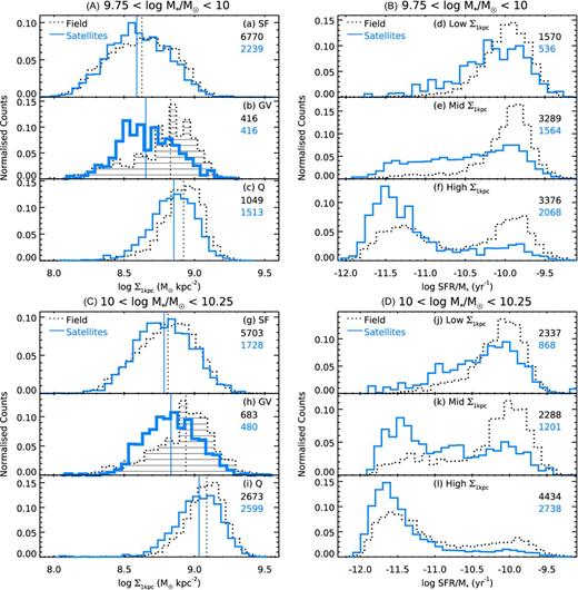
Left-hand column: one-dimensional distributions of Σ*,1kpc in the mass range 9.25 < log M*/M⊙ < 10 (A) and 10 < log M*/M⊙ < 10.25 (C), in three star-forming classes corresponding to the divisions in Fig. 2. Right-hand column: distributions of sSFR in three bins of Σ*,1kpc in the same mass ranges. The divisions between ‘Low’, ‘Mid’ and ‘High’ Σ*,1kpc are log Σ*,1kpc/(M⊙kpc−2) = 8.4 and 8.7 for the lower mass bin, and log Σ*,1kpc/(M⊙kpc−2) = 8.7 and 8.9 for the more massive bin. The vertical lines in the left-hand panels show the medians of each histogram. The histograms are normalized by number density. These histograms confirm these features seen in Fig. 4: GV satellites lie at lower Σ*,1kpc than GV field galaxies by about 0.2 dex for the lowest mass bin (b and h); Q satellites have a lower range Σ*,1kpc than the field (c and i); the peak sSFR of SF and Q satellites is lower than that of SF field galaxies (d–f and j–l).
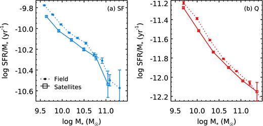
The median sSFR as a function of M* for satellites (square symbols connected by solid lines) and field galaxies (circles connected by dotted lines). The two panels include only SF (a) and Q (b) galaxies as defined in Fig. 2. Error bars are bootstrap errors. Satellites have lower sSFR than field galaxies by about 0.1 dex at the same mass and star formation class. In particular, the main sequence is lower for satellites than for field galaxies.
Note that these observations will be missed in simple studies of the quenched fraction rather than the bivariate distribution in the sSFR–Σ*,1kpc plane.
The lower panels of Fig. 4 show that most of these differences between field and satellite galaxies listed above are present also at higher masses, but these differences are much smaller than for the lowest bin of M*. The GV bridge of satellites is shifted towards lower in Σ*,1kpc relative to the field, and the centroids of the SF and Q populations are shifted to lower sSFR and lower Σ*,1kpc, respectively (except perhaps for the most massive Q satellites), but these differences are smaller than 0.1 dex.
Fig. 5(A) and (B) flatten the information in Fig. 4(a) and (b) into one-dimensional distributions of Σ*,1kpc in three SF classes (panels a, b and c) and sSFR in three bins of Σ*,1kpc (panels d, e and f). Satellite histograms are in blue while the field histograms are in black. SF, GV and Q galaxies are defined by the dividing lines in Fig. 2. (Our results are not sensitive to reasonable variations in slope and zero-points of these divisions.) The histograms are normalized by their total number densities. Fig. 5(C) and (D) show the second mass bin (10 < log M*/M⊙ < 10.25). For brevity, we show only our two lowest bins (9.75 < log M*/M⊙ < 10 and 10 < log M*/M⊙ < 10.25), where the effects are largest.
Fig. 5 confirms the same features described above. The GV for satellites (bold blue histogram in panels b and h) is peaked at lower Σ*,1kpc (by about 0.2 dex for the lowest masses) than the GV field galaxies (dotted black histogram) which corresponds to the shift of the GV bridge in Fig. 4(b) and (d). The Q satellites are also weighted towards lower Σ*,1kpc than the field but not as much as the GV (∼0.1 dex – panels c and i of Fig. 5). The total Σ*,1kpc distribution for satellites (adding up the solid histograms) is weighted towards higher in Σ*,1kpc than the total distribution for field galaxies (not shown here). (This is related to the morphology–density relation; Holmberg 1940; Dressler 1980.) This is the combined effect of quenching being correlated with high Σ*,1kpc and the satellites having higher quenched fraction than the field. However, at fixed sSFR, GV and Q satellites have lower Σ*,1kpc than GV and Q galaxies in the field.
It should be noted that even within a narrow mass bin, Σ*,1kpc is correlated with M*. Since the mass function of satellites is bottom-heavier than that of the field (Peng et al. 2010), we checked if the Σ*,1kpc differences between satellites and the field might be due to the mass differences. We find that the differences in the mass distributions (≲0.03 dex) are too small to account for the differences we see in Σ*,1kpc. (The slopes of the Σ*,1kpc–M* relation for SF and Q galaxies are ∼0.9 and 0.65, respectively – see also Barro et al. 2015.)
The right-hand panels of Fig. 5 show that at fixed Σ*,1kpc, the SF peak of sSFR bimodality is slightly lower for satellites than in the field by about 0.1 dex. In these panels, the tail of the SF satellites seems to fill the GV. In fact, for the field, galaxies with mid-range, Σ*,1kpc that are quenched, are relatively rare, whereas quenched satellites are more than half the satellite population with mid-range Σ*,1kpc (panels e and k). The quenched peaks, where present, are also lower in sSFR for satellites than the field.
We also show this lowering of the sSFR explicitly in Fig. 6, which shows the median sSFR as a function of M* for satellites and field galaxies. This figure shows that SF and Q satellites have lower sSFR than field galaxies at the same mass. In particular, the SF ‘main sequence’ of satellites is systematically lower than that of field galaxies by about 0.05–0.1 dex, compared to a spread of 0.2–0.3 dex for the whole main sequence (depending on how the main sequence is defined). This difference also disappears around M* ∼ 1010.7 M⊙ and higher.
Note that these findings are features of the sSFR–Σ*,1kpc plane, but we checked that a similar analysis using other independent measures of morphology/structure (bulge mass and §érsic n) produces similar results.
3.2 Structural properties of satellites within the halo environment
While the above plots have compared field and satellite galaxies at the same stellar mass, satellites are subject to two other potentially influential parameters, namely, the mass of the halo in which they reside and their distance from the centre of that halo. Since halo masses are assigned based on the total stellar mass of all members in a group, a satellite must lie in a halo at least twice as massive as a field galaxy of the same M*.
To disentangle environment, morphology and structure from each other, we divide the D–Mh plane into four quadrants at Mh = 1013.5 M⊙ and log D = −0.6 (Rproj ∼ 0.25Rvir), and study the sSFR-Σ*,1kpc distribution in these different environments. (These divisions were chosen because the quenched fraction depends most strongly on D above this mass, and most strongly on Mh below this distance, as seen in fig. 10b of Woo et al. 2013.) These distributions are shown in different mass bins in Figs 7 and 8 (Again, the raw unweighted points are shown in the Appendix, Figs A2 and A3.) In these figures, ‘Near’ and ‘Far’ refer to satellites with log D less than and greater than −0.6, while ‘low Mh’ and ‘high Mh’ refer to satellites in host haloes less than or greater than 1013.5 M⊙. The GV, as defined in Fig. 2, lies roughly between the two horizontal lines, and the vertical line marks the median Σ*,1kpc of the field GV for reference.
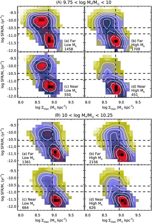
The distribution of satellite galaxies in the sSFR–Σ*,1kpc plane in four panels representing different environments, for two mass bins (A and B). ‘Near’ and ‘Far’ refer to log D less than or greater than −0.6 (or Rproj ∼ 0.25Rvir). ‘Low Mh’ and ‘High Mh’ refer to haloes less massive than or more massive than 1013.5 M⊙. Satellites in the GV as defined in Fig. 2 lie roughly between the two horizontal lines. For reference, the vertical line marks the median Σ*,1kpc for the field GV. The contours represent the logarithmic number density of the population in each panel and are separated by 0.2 dex. The colour scale is normalized such that dark red represents the highest number density in that panel. The sample size of each panel is indicated in the bottom corner. The shift of the GV bridge, the lowering of sSFR for the SF satellites and the extension of Q satellites towards lower Σ*,1kpc compared with the field is driven by high Mh and low D.
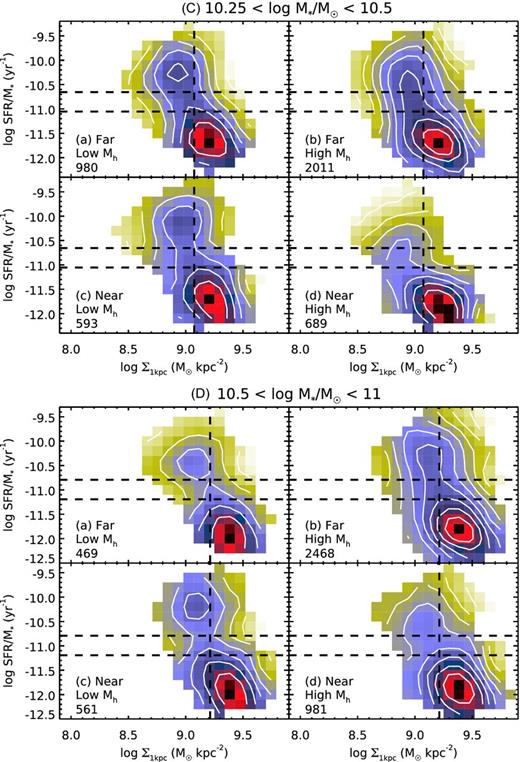
The distribution of satellite galaxies in the sSFR–Σ*,1kpc plane in four panels representing different environments, for two mass bins (C and D). ‘Near’ and ‘Far’ refer to log D less than or greater than −0.6 (or Rproj ∼ 0.25Rvir). ‘Low Mh’ and ‘High Mh’ refer to haloes less massive than or more massive than 1013.5 M⊙. Satellites in the GV as defined in Fig. 2 lie roughly between the two horizontal lines. For reference, the vertical line marks the median Σ*,1kpc of the field GV. The contours represent the logarithmic number density of the population in each panel and are separated by 0.2 dex. The colour scale is normalized such that dark red represents the highest number density in that panel. The sample size of each panel is indicated in the bottom left corner. The massive satellites here continue the trends seen in the two lower mass bins, but more weakly than the less massive satellites.
Figs 7 and 8 show that for satellites in all environments, low sSFR is associated with high Σ*,1kpc as is the case for the field (Fig. 4). Σ*,1kpc for Q galaxies is always about 0.2–0.3 dex higher than that of SF galaxies. The satellites in Fig. 7(a), i.e. those far from their group centres and in less massive haloes, are the most similar to the field (Fig. 4a). It is the panel with the lowest quenched fraction and the SF distribution is wide in Σ*,1kpc, as in the field. These may only be loosely bound to their groups. It is also quite possible that many of these are actually field galaxies misclassified by the group finder. However, despite these uncertainties, a comparison between Fig. 7(a) and Fig. 4(a) shows that even this population of satellites is not the same as the field population. The same phenomena observed in Fig. 4 when comparing the field and the satellites are also present when comparing this subsample of satellites: the GV bridge for satellites is shifted towards lower Σ*,1kpc, the SF and Q populations of satellites are shifted towards lower sSFR and the spread of Σ*,1kpc for the Q satellites is elongated towards lower Σ*,1kpc.
Comparing the other panels of Figs 7 and 8, the quenched fraction clearly depends on both Mh and D. This can be thought of as the zero-order effect seen in Woo et al. (2013) and other studies of the quenched fraction (Balogh et al. 2004; Hansen et al. 2009; Peng et al. 2010; Wetzel et al. 2012 and others mentioned in Section 1.2). The higher order effects, i.e. the differences between satellites and the field seen in Fig. 4 (listed in Section 3.1), seem also to depend on these measures of environment. In fact, the position of the GV seems to shift more towards lower Σ*,1kpc with more extreme environments (higher Mh and lower D) just as the quenched fraction increases.
Here we explore this observation further. We take the quenched fraction fq in each of the four panels of Fig. 7(A) and (B) and put this number on the x-axis of Fig. 9(b). Thus, we are treating fq as a proxy for the ‘environment’ even though the environment is a function of our two orthogonal measures (Mh and D). The y-axis is the median Σ*,1kpc of the GV population in that panel. We also do this for the additional ‘environment’ of the field, adding the quenched fraction and GV position of Fig. 4(a)–Fig. 9(b). These five environments are represented by the five different symbols, while the colours represent different mass bins. Panels a and c of Fig. 9 show the medians of Σ*,1kpc for the SF and Q populations as well. (Note that for this figure, we used the mass-complete redshift cuts described in Section 2 in order to compare quenched fractions.) Fig. 9(b) shows that within a mass bin, the median Σ*,1kpc of the GV declines smoothly with our proxy for the environment, so that the GV galaxies in the most extreme environment have a Σ*,1kpc that is ∼0.2 dex lower than the field. Σ*,1kpc of the GV declines with environment at a similar rate in each mass bin. The lines, which have a fixed slope of −0.5, are good fits to each bin. The median Σ*,1kpc for SF and Q galaxies also declines somewhat with environment, but this is not as strong as the trend for the GV. The maximum difference in Σ*,1kpc between the environments is ∼0.1 dex. (The lines in panels a and c are fit vertically with a slope of −0.2.)
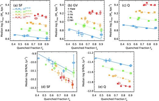
a–c: the median log Σ*,1kpc of the SF (a), GV (b) and Q (c) populations in four mass bins as a function of the quenched fraction of different environments (labelled). d, e: the median sSFR of the SF (d) and Q (e) populations as a function of M* and environment (represented by fq). ‘FL’, ‘FH’, ‘NL’ and ‘NH’ refer to satellites in panels a, b, c and d of Figs 7 and 8. Error bars represent bootstrap errors. The lines are fitted to have fixed slopes in each panel: −0.2 (a and c), −0.5 (b), −0.45 (d) and −0.35 (e). The median log Σ*,1kpc of the GV decreases regularly with quenched fraction, which is our proxy for the environment.
Panels d and e of Fig. 9 show the median sSFR of the SF and Q populations as a function of fq, split into the same mass and environment bins. The lines have a fixed slope of −0.45 and −0.35 for the SF and Q populations, respectively. These panels show that the median sSFR also declines smoothly with our proxy for the environment so that the maximum difference in sSFR between environments is ∼0.15 dex (for both SF and Q galaxies). We noted that the variations of the features of the sSFR–Σ*,1kpc diagram with the environment decrease with M*. Indeed, the red points in Fig. 9 could just as well be fit with horizontal lines. However, the overall pattern in Fig. 9 suggests that the weaker environmental dependence of sSFR–Σ*,1kpc features at high masses (e.g. Fig. 4g and h) can be attributed simply to the higher fq of all massive galaxies. Thus, it appears that the main features of the sSFR–Σ*,1kpc diagram, i.e. the positions of the SF, GV and Q populations, are well predicted by the environment (fq) and M*.
4 DISCUSSION
We have shown that the sSFR–Σ*,1kpc diagram is a promising diagnostic of the differences in the quenching processes among different populations of galaxies. We have studied this diagram as a function of three population variables: stellar mass, halo mass (for satellites) and radial location within haloes (also for satellites). Different features are seen, which may ultimately be linked to the different quenching mechanisms that are thought to affect galaxies in different environments.
The basic result is that the sSFR–Σ*,1kpc diagram varies with environment: the diagram for field galaxies differs from that of all satellites and the diagrams for satellites differ depending on group-centric distance and halo mass. In particular, we find the following.
‘Environment’ can be approximated by the quenched fraction. The environment of galaxies is, in principle, a function of both group-centric distance and the mass of the host halo. We confirm what has been seen in many studies that the quenched fraction increases with Mh, and in massive haloes, with decreasing D. However, we find that these two quantities conspire such that a single quantity, the quenched fraction of the population (including in the field), accurately predicts the rest of the distribution of galaxies in the sSFR–Σ*,1kpc plane. In other words, using the quenched fraction as a proxy for the environment, the following features are seen to vary smoothly with that measure.
The median value of Σ*,1kpc in the GV decreases smoothly with the quenched fraction of the environment. In other words, the position of the GV bridge between the SF and Q populations in the sSFR–Σ*,1kpc diagram shifts towards lower Σ*,1kpc by as much as 0.2 dex (at M* = 109.75–10) for satellites compared to the field and for satellites in more massive haloes and lower cluster-centric distance.
The sSFR ridge-line of SF galaxies falls slightly with increasing quenched fraction of the environment. This is a small effect (∼0.1 dex) but it is systematic over a large range of M*.
The median Σ*,1kpc of quenched galaxies in a given mass bin is always higher than the SF population by about 0.2–0.3 dex. The exact value also varies slightly with environment (as measured by the quenched fraction), but the variation is smaller than the variation in the median Σ*,1kpc of the GV or of the sSFR of the SF population.
The magnitude of the above variations with environment depends on M*. The quenched fraction, median Σ*,1kpc of the GV and sSFR of the SF population, vary significantly with environment for low-mass galaxies (M* ≲ 1010 M⊙) but much less for the most massive galaxies (M* ≳ 1010.5 M⊙). This may be a reflection of the uniformly high-quenched fractions for intermediate- and high-mass field galaxies (Fig. 9). Since, at a given mass, the number of field galaxies is about twice the number of satellites, most quenched galaxies of mass M* ≳ 1010.5 M⊙ likely quenched as field galaxies, some of which later became quenched satellites. Galaxies of lower mass, on the other hand, have a quenched fraction that is more than double the quenched fraction in the field, indicating that a significant portion of these satellites quenched as satellites.
These results are consistent with the expectation of an environmentally induced quenching track that occurs in clusters today and that is in addition to the quenching that occurs in the field (Fig. 1). In the field, it appears that galaxies must have high Σ*,1kpc relative to the rest of the SF main sequence (by about 0.2–0.3 dex) in order to start quenching (i.e. to bring them to the GV; this is consistent with Cheung et al. 2012; Fang et al. 2013; Barro et al. 2015). Since external influences are presumably lacking in the field, quenching must occur due to the properties of the galaxy itself or its own halo, e.g. the mass of its halo, AGN state, stability of the disc, etc. Referring to these collectively as ‘self-quenching’, the sSFR–Σ*,1kpc diagram in the field indicates that high Σ*,1kpc is associated with self-quenching.
In contrast, the distribution of Σ*,1kpc for satellites in the GV is more similar to the distribution of Σ*,1kpc on the SF main sequence (blue histograms in Fig. 5, comparing a to b and g to h), indicating that quenching in clusters is not associated with high Σ*,1kpc. This is consistent with the influence of external factors that quench (at least to the GV) regardless of Σ*,1kpc or without altering Σ*,1kpc. Furthermore, the small suppression of the sSFR of the SF population, also independent of Σ*,1kpc (Fig. 5 B and D), may be an indication that the start of quenching occurs immediately upon becoming a satellite. Our finding that the features of the sSFR–Σ*,1kpc diagram vary smoothly with the environment (via fq) may reflect the decreasing relative importance of self-quenching versus external processes in more extreme environments.
4.1 Why is Σ*,1kpc of quenched Galaxies always high?
While our findings indicate that satellite quenching begins at a wide range of Σ*,1kpc, satellites that have more or less finished their quenching all have the highest Σ*,1kpc (compared to SF and GV galaxies) in a given mass bin. As detailed in Section 1, it has been demonstrated that quenching is strongly associated with early-type morphology for the galaxy population as a whole, which is dominated by field galaxies. However, we have shown here that even in the densest environments, there are almost no quenched satellites with low Σ*,1kpc. This is a surprising result in light of the various proposed satellite quenching mechanisms. This result rules out the simple vertically downwards quenching track on the sSFR–Σ*,1kpc diagram, such as might be expected, for example, from the cut-off of accretion (Dekel & Birnboim 2006) and the stripping of cold gas via ram pressure. Both of these scenarios are expected to quench satellites quickly regardless of Σ*,1kpc (although see McCarthy et al. 2008). To explain high Σ*,1kpc in quenched satellites, we discuss here some of the remaining scenarios which can be divided into two classes: those that involve the creation of new stars in the central kpc and those in which the Σ*,1kpc value of individual galaxies remains intact.
Mechanisms for satellite quenching that involve the creation of new stars include galaxy–galaxy interactions (sometimes called ‘harassment’), which build the density in the inner kpc with each successive interaction (Lake, Katz & Moore 1998). Ram pressure, usually thought to strip gas from a galaxy, can also potentially compress gas in the inner regions. Dekel et al. (in preparation) estimate that starting at 0.5Rvir, ram pressure can increase Σ*,1kpc by up to a factor of 2 (what is needed to explain the sSFR–M* diagram) if the gas fraction is ∼0.5. Such gas fractions are seen in lower mass galaxies than studied here, or at higher z, and thus this process may be relevant for those regimes. However, the galaxies in the GV observed here likely have much lower gas fractions, and so ram pressure compression may not be responsible for the high Σ*,1kpc of quenched satellites relative to GV satellites observed here.
Tidal compression may prove to be more promising. Tidal forces in haloes with shallow profiles are compressive and can increase Σ*,1kpc by a factor of 2 even with gas fractions as low as 0.1 (Dekel, Devor & Hetzroni 2003; Dekel et al. in preparation). However, such tidal compression is only efficient within 0.1Rvir.
In any case, our results imply that any quenching scenario that increases Σ*,1kpc must begin quenching (bringing the galaxies from the SF to the GV) before the increase of Σ*,1kpc. This is indicated by the fact that the satellite quenching tracks increase in Σ*,1kpc only after galaxies have passed through the GV and are en route to the quenched region.
It is also possible to explain the high apparent Σ*,1kpc of quenched galaxies without increasing Σ*,1kpc in individual galaxies. This is possible if galaxies lose mass during quenching and thus move from one mass bin to another. For example, tidal stripping of a satellite in a higher mass bin can strip both gas and stars, potentially lowering M* significantly from the infall value (as much as 30–40 per cent or more per pericentre passage – Zentner & Bullock 2003; Taylor & Babul 2004), but will leave Σ*,1kpc intact. Indeed, comparing the sSFR–Σ*,1kpc diagrams in Fig. 4, Σ*,1kpc of the GV for satellites is always comparable to the Σ*,1kpc of the Q population in the immediately lower mass bin, supporting the plausibility of the stripping scenario. The position of the GV in the sSFR–Σ*,1kpc diagrams would imply that the start of quenching occurs before the stripping, which is reasonable considering that tidal stripping is most efficient at the orbital pericentre. This would be in line with the findings of Pasquali et al. (2010) who find that the mass–metallicity relation of satellites is offset towards lower mass.
One additional effect that can explain the high Σ*,1kpc of quenched galaxies without increasing Σ*,1kpc is one that has received little attention so far – namely, ‘progenitor bias’. The idea is that at any given M*, Q galaxies that quench at earlier times are expected to be denser, on average, than at later times, simply because progenitor SF galaxies, their dark matter haloes and the whole Universe are denser at earlier epochs (e.g. Valentinuzzi et al. 2010; Carollo et al. 2013a; Poggianti et al. 2013; Lilly & Carollo 2016). Thus, the sSFR–Σ*,1kpc diagrams for the field population can be explained by the gradual displacement of the GV bridge towards lower Σ*,1kpc over time, filling the lower end of the Q cloud. The evolution of the Σ*,1kpc versus M* relation of the whole Q galaxy population averaged over all environments shows a decrease of ∼0.3 dex in Σ*,1kpc since a redshift of z ∼ 3 (Barro et al. 2015), which well agrees with the width of the Q cloud.
As for the satellites, the morphology of the sSFR–Σ*,1kpc diagram could arise from the cumulative effects of (1) a pre-dominant role of field-like self-quenching at early epochs and (2) the switching-on of satellite-quenching at later epochs, which quenches at lower Σ*,1kpc. (See also Gallart et al. 2015 who suggest that dwarf satellite morphologies are determined at birth.)
It is possible that the Σ*,1kpc-increasing mechanisms (such as those described above) and the effect of progenitor bias work in concert. How important these effects are can at least, in part, be tested through direct measurement of sSFR–Σ*,1kpc diagrams at earlier epochs and their stellar populations (work in progress).
In summary, we have used the sSFR–Σ*,1kpc diagram as a useful diagnostic of quenching among different populations of galaxies. The power of Σ*,1kpc to predict quenching that has been seen in bulk populations of galaxies is confirmed when galaxies are divided up into field versus satellites and satellites in different haloes and at different group-centric distances. The location of the transitioning galaxies (i.e. the GV) in the sSFR–Σ*,1kpc diagram varies smoothly with the environment, Σ*,1kpc being lower for satellites in larger haloes and at smaller radial distances within the same-mass haloes. We interpret this shift as indicating the relative importance in different environments of the field quenching track versus the cluster quenching track. In all environments, the Q population always has high Σ*,1kpc relative to their masses. We proposed two types of scenarios to explain the high Σ*,1kpc of Q satellites relative to the low Σ*,1kpc of GV (and SF) satellites. One class of scenarios involves the creation of new stars in the inner kpc (harassment, ram pressure compression and tidal compression) while the other class does not involve such star formation (tidal stripping causing significant mass-loss and progenitor bias). It is the goal of future work to distinguish between these possibilities.
Acknowledgments
We acknowledge the helpful and stimulating discussions with Guillermo Barro, Colin DeGraf, Marla Geha, Will Hartley, Andrew Hearin, David Koo, Simon Lilly, Nir Mandelker, Joel Primack, Aldo Rodgriquex-Puebla, Kevin Schawinski, Rachel Sommerville, Benny Trakhtenbrot, and Frank van den Bosch. We acknowledge support from the Swiss National Science Foundation. SF acknowledges support from the National Science Foundation grant AST-08-08133.
Funding for the SDSS and SDSS-II has been provided by the Alfred P. Sloan Foundation, the Participating Institutions, the National Science Foundation, the US Department of Energy, the National Aeronautics and Space Administration, the Japanese Monbukagakusho, the Max Planck Society, and the Higher Education Funding Council for England. The SDSS Web Site is http://www.sdss.org/. The SDSS is managed by the Astrophysical Research Consortium for the Participating Institutions. The Participating Institutions are the American Museum of Natural History, Astrophysical Institute Potsdam, University of Basel, University of Cambridge, Case Western Reserve University, University of Chicago, Drexel University, Fermilab, the Institute for Advanced Study, the Japan Participation Group, Johns Hopkins University, the Joint Institute for Nuclear Astrophysics, the Kavli Institute for Particle Astrophysics and Cosmology, the Korean Scientist Group, the Chinese Academy of Sciences (LAMOST), Los Alamos National Laboratory, the Max-Planck-Institute for Astronomy (MPIA), the Max-Planck-Institute for Astrophysics (MPA), New Mexico State University, Ohio State University, University of Pittsburgh, University of Portsmouth, Princeton University, the United States Naval Observatory, and the University of Washington.
REFERENCES
APPENDIX:
Figs A1–A3 are the same as Figs 4, 7 and 8, except that they show individual points instead of weighted contours.
sSFR versus Σ*,1kpc, in four bins of M* for field galaxies and satellites. This is the same as Fig. 4 but using the raw unweighted and unsmoothed points. The GV, as defined in Fig. 2, lies roughly between the two horizontal lines. For reference, the vertical line marks the median Σ*,1kpc of hte field GV. The sample size of each panel is indicated in the bottom corner.
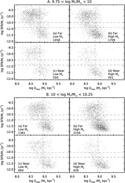
The distribution of satellite galaxies in the sSFR–Σ*,1kpc plane in four panels representing different environments in two mass bins (A and B). This is the same as Fig. 7 but using the raw unweighted and unsmoothed points. ‘Near’ and ‘Far’ refer to log D less than or greater than −0.6 (or Rproj ∼ 0.25Rvir). ‘Low Mh’ and ‘High Mh’ refer to haloes less massive than or more massive than 1013.5 M⊙. Satellites in the GV as defined in Fig. 2 lie roughly between the two horizontal lines. For reference, the vertical line marks the median Σ*,1kpc of the field GV. The sample size of each panel is indicated in the bottom corner.
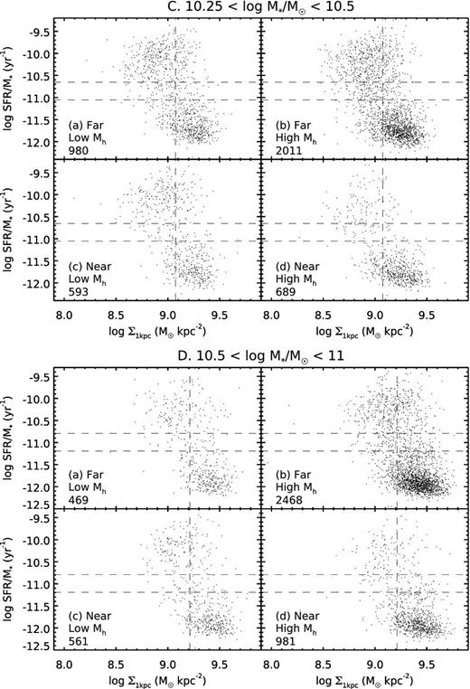
The distribution of satellite galaxies in the sSFR–Σ*,1kpc plane in four panels representing different environments in two mass bins (C and D). This is the same as Fig. 8 but using the raw unweighted and unsmoothed points. ‘Near’ and ‘Far’ refer to log D less than or greater than −0.6 (or Rproj ∼ 0.25Rvir). ‘Low Mh’ and ‘High Mh’ refer to haloes less massive than or more massive than 1013.5 M⊙. Satellites in the GV as defined in Fig. 2 lie roughly between the two horizontal lines. For reference, the vertical line marks the median Σ*,1kpc of the field GV. The sample size of each panel is indicated in the bottom corner.
