


Abstract
The discovery of GeV gamma-rays from classical novae indicates that shocks and relativistic particle acceleration are energetically key in these events. Further evidence for shocks comes from thermal keV X-ray emission and an early peak in the radio light curve on a time-scale of months with a brightness temperature which is too high to result from freely expanding photoionized gas. Paper I developed a one-dimensional model for the thermal emission from nova shocks. This work concluded that the shock-powered radio peak cannot be thermal if line cooling operates in the post-shock gas at the rate determined by collisional ionization equilibrium. Here we extend this calculation to include non-thermal synchrotron emission. Applying our model to three classical novae, we constrain the amplification of the magnetic field ϵB and the efficiency ϵe of accelerating relativistic electrons of characteristic Lorentz factor γ ∼ 100. If the shocks are radiative (low velocity vsh ≲ 1000 km s−1) and cover a large solid angle of the nova outflow, as likely characterize those producing gamma-rays, then values of ϵe ∼ 0.01–0.1 are required to achieve the peak radio brightness for ϵB = 10−2. Such high efficiencies exclude secondary pairs from pion decay as the source of the radio-emitting particles, instead favouring the direct acceleration of electrons at the shock. If the radio-emitting shocks are instead adiabatic (high velocity), as likely characterize those responsible for the thermal X-rays, then much higher brightness temperatures are possible, allowing the radio-emitting shocks to cover a smaller outflow solid angle.
INTRODUCTION
Classical and symbiotic novae are luminous transients, powered by runaway thermonuclear burning of a hydrogen-rich layer accreted from a binary companion (e.g. Gallagher & Starrfield 1978; Starrfield et al. 2000; Townsley & Bildsten 2005; Yaron et al. 2005; Casanova et al. 2011). The resulting energy release causes the white dwarf atmosphere to inflate, ejecting ∼10−5–10−4 M⊙ of CNO-enriched matter at hundreds to thousands of kilometres per second (e.g. Seaquist et al. 1980; Shore 2012).
Radio and optical imaging (Chomiuk et al. 2014b; Schaefer et al. 2014), and optical spectroscopy (Ribeiro, Munari & Valisa 2013; Shore et al. 2013), suggests that a nova outburst proceeds in at least two stages (Fig. 1). The runaway is first accompanied by a low-velocity outflow concentrated in the equatorial plane of the binary, perhaps influenced by the gravity of the companion star, as occurs in common envelope phases of stellar evolution (e.g. Livio et al. 1990; Lloyd, O'Brien & Bode 1997). Given the uncertain nature of the slow ejecta, we use the agnostic term ‘dense external shell’ (DES; Metzger et al. 2014).
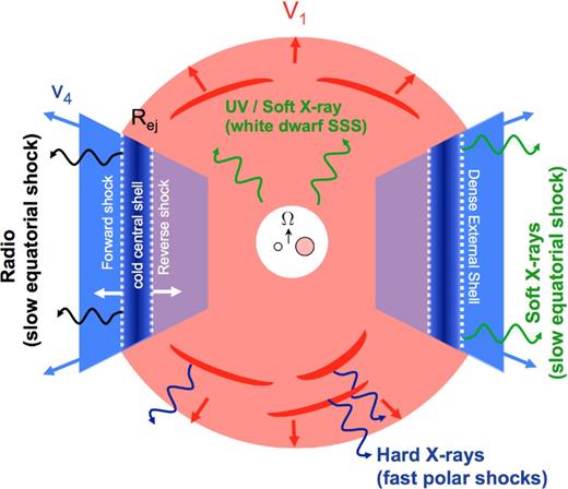
Proposed scenario for the locations of X-ray and radio-emitting shocks. A slow outflow is ejected first, its geometry shaped into an equatorially concentrated torus (blue). This is followed by a faster outflow or continuous wind with a higher velocity and more spherical geometry (red). The fast and slow components collide in the equatorial plane, producing powerful radiative shocks (Fig. 2) which are responsible for the gamma-ray emission on time-scales of weeks and the non-thermal radio emission on a time-scale of months. Adiabatic internal shocks within the fast, low-density polar outflow power hard ≫keV thermal X-rays and possibly radio emission at very early times. Slower equatorial shocks produce the non-thermal radio peak on a time-scale of months and softer X-rays (kT ≲ keV), which are challenging to detect due to their lower luminosity and confusion with supersoft X-rays from the white dwarf. The direction of the binary orbital angular velocity Ω is indicated by an arrow.
The outflowing DES is then followed by a more continuous wind (e.g. Bath & Shaviv 1976) with a higher velocity and a more spherical geometry. A collision between this fast outflow and the slower DES results in strong internal shocks, which are most powerful near the equatorial plane where the density contrast is largest. If the fast component expands relatively unimpeded along the polar direction, this creates a bipolar morphology (Chomiuk et al. 2014b; Metzger et al. 2015). Such a scenario does not exclude fast shocks within the polar region, characterized by lower densities and hard X-ray emission (Fig. 1).
Several lines of evidence support shocks being common features of nova outbursts. Nova optical spectra exhibit complex absorption lines with multiple velocity components (e.g. Friedjung & Duerbeck 1993; Williams et al. 2008; Williams & Mason 2010). In addition to broad P Cygni lines indicating high-velocity ≳1000 km s−1 matter, narrower absorption features (≈500–900 km s−1) are observed near optical maximum and may be created within the DES. A large fraction of novae show such narrow lines. This indicates that the absorbing material has a high covering fraction (Williams & Mason 2010) and hence is likely to impact the faster P Cygni outflow.
Many novae are accompanied by thermal X-ray emission of luminosity LX ∼ 1033–1035 erg s−1 and temperatures ≳keV (e.g. Lloyd et al. 1992; O'Brien, Lloyd & Bode 1994; Orio 2004; Sokoloski et al. 2006; Ness et al. 2007; Mukai, Orio & Della Valle 2008; Krauss et al. 2011; Schwarz et al. 2011; Chomiuk et al. 2014b; see Osborne 2015 for a summary of Swift observations). This emission is too hard to be thermal radiation from the white dwarf surface (Wolf et al. 2013), but is readily explained as free–free emission from ≳1000 km s−1 shocks (e.g. Mukai & Ishida 2001). The X-ray emission is often delayed by weeks or longer after the optical maximum, perhaps due to absorption by the DES (Metzger et al. 2014).
Although the presence of shocks in novae have been realized for some time, their energetic importance was only recently revealed by the Fermi-LAT discovery of ≳100 MeV gamma-rays, coincident within days of the optical peak and last for weeks (Ackermann et al. 2014). Gamma-rays were first detected in the symbiotic nova V407 Cyg 2010, in which the target material for the shocks could be understood as the dense wind of the companion red giant (Abdo et al. 2010; Vaytet et al. 2011; Martin & Dubus 2013). However, six additional novae have now been detected by Fermi-LAT, at least four of which show no evidence for a giant companion and hence were likely ordinary classical novae with main-sequence (MS) companions. The DES is clearly present even in binary systems that are not embedded in the wind of an M giant or associated with recurrent novae, supporting the internal shock scenario.
The high gamma-ray luminosities Lγ ∼ 1035–1036 erg s−1 require shocks with kinetic powers which are at least two orders of magnitude larger, i.e. Lsh ∼ 1037–1038 erg s−1, approaching the bolometric output of the nova (Metzger et al. 2015). Gamma-rays are produced by the decay of neutral pions created by collisions between relativistic protons and ambient protons in the ejecta (hadronic scenario), or by inverse Compton or bremsstrahlung emission from relativistic electrons (leptonic scenario). Hadronic versus lepton emission scenarios cannot be distinguished based on the gamma-ray spectra alone (Ackermann et al. 2014), although Metzger et al. (2015) cite evidence in favour of a hadronic scenario.
Additional evidence for shocks comes at radio wavelengths. Novae produce thermal radio emission from the freely expanding photoionized ejecta of temperature ∼104 K, which peaks as the ejecta becomes optically thin to free–free absorption roughly a year after the optical outburst (Seaquist & Bode 2008). However, a growing sample of novae show an additional peak in the radio emission at earlier times (≲100 d; Taylor et al. 1987; Krauss et al. 2011; Chomiuk et al. 2014b; Weston et al. 2016b; Fig. 4) with brightness temperatures 105–106 K higher than that of photo-ionized gas. This additional early radio peak requires sudden heating of the ejecta (e.g. Lloyd, O'Brien & Bode 1996; Metzger et al. 2014) or non-thermal emission (Taylor et al. 1987; Weston et al. 2016b), in either case implicating shocks.
Metzger et al. (2014, hereafter Paper I) developed a one-dimensional model for the forward-reverse shock structure in novae and its resulting thermal X-ray, optical, radio emission. This initial work provided an acceptable fit to the radio light curves of the gamma-ray nova V1324 Sco, under the assumption that the dominant cooling behind the shock was provided by free–free emission. However, for low-velocity shocks ≲103 km s−1, line cooling of the CNO-enriched gas can greatly exceed free–free cooling. For cooling rates determined by collisional ionization equilibrium (CIE), this additional cooling reduces the peak brightness temperature of thermal models to values ≲104 K, which are too low to explain the early radio peak, unless line cooling is suppressed by non-local thermodynamic equilibrium effects.
In this work (Paper II), we extend the Paper I model to include non-thermal synchrotron radio emission, which we demonstrate can explain the observed emission, even for low shock velocities. In addition to providing information on the structure of the ejecta and the nova outburst mechanism, synchrotron emission provides an alternative probe of relativistic particle acceleration in these events, complementary to that obtained from the gamma-ray band. In leptonic scenario, relativistic electrons accelerated directly at the shock power the radio emission. Radio-emitting e± pairs are also produced in hadronic scenarios by the decay of the charged pions. Radio observations can in principle help disentangle leptonic from hadronic models.
This paper is organized as follows. We begin with an overview of shocks in novae (Section 2), including the collision dynamics, observational evidence for shocks, the analytic condition for radio maximum, the radiative versus adiabatic nature of the shock, and thermal X-ray emission. We also summarize the most important variables used throughout the paper in Table 1. In Section 3, we describe key features of synchrotron emission, including leptonic and hadronic sources of non-thermal particles and their cooling. In Section 4, we provide a detailed description of our model for radio emission from the forward shock. In Section 5, we describe our results, including analytic estimates for brightness temperature, and fits to the radio light curves of three novae: V1324 Sco, V1723 Aql, and V5589 Sgr. In the discussion (Section 6), we use the radio observations to constrain the acceleration efficiency of relativistic particles and magnetic field amplification in the shocks and their connection to gamma-ray emission. We also discuss outstanding issues, including the unexpectedly monochromatic light curve of V1723 Aql and the role of adiabatic X-ray producing shocks. In Section 7, we summarize our conclusions.
Commonly used variables and their definitions.
| Variable | Definition |
|---|---|
| v1 | Velocity of fast outflow (Fig. 2) |
| v4 | Velocity of DES |
| n1 | Density of (unshocked) fast outflow |
| n4 | Density of (unshocked) DES |
| T4 | Temperature of DES in the photoionized layer just ahead of the shock |
| T3 | Temperature immediately behind the forward shock |
| n3 | Density immediately behind forward shock |
| vshock | Velocity of forward shock in the white dwarf frame |
| vshell | Velocity of central shell in the white dwarf frame |
| |$\tilde{v}_{\rm f}\equiv v_{{\rm shock}}-v_4 \equiv 10^8 v_8\, {\rm cm\,s}^{-1}$| | Velocity of the shock in the frame of the DES |
| H = 1014H14 cm | Density scaleheight of DES |
| Tb | Observed brightness temperature, corrected for pre-shock screening by the photoionized layer |
| τff, 4 | Free–free optical depth of unshocked DES |
| αff, 4 | Free–free absorption coefficient of unshocked DES |
| tcool | Cooling time of gas in the post-shock region |
| Δion | Thickness of ionized layer ahead of the shock (equation 5) |
| η3 ≡ tcool/tfall | Cooling efficiency: ratio of post-shock cooling time-scale to shock expansion time down the density gradient of the DES (equation 18) |
| npk, Δ | Density of unshocked DES at time of radio peak (τff,4 = 1) for the case when Δion < H (equation 12, upper line) |
| npk, H | Density of unshocked DES at time of radio peak (τff,4 = 1) for the case when Δion > H (equation 12, lower line) |
| Mej | Total ejecta mass |
| Rsh | Radius of cool central shell ∼ radius of shock |
| fEUV = 0.1fEUV, -1 | Fraction of shock power placed into hydrogen-ionizing radiation |
| ϵp = 0.1ϵp, −1 | Fraction of shock power placed into relativistic protons |
| ϵe | Fraction of shock power placed into relativistic electrons and positrons |
| γpk | Lorentz factor of the electrons or positrons which determine the synchrotron emissivity at the radio peak |
| Tν | Brightness temperature of emission at generic location behind the shock |
| Tν, sync | Brightness temperature of synchrotron emission (equation 38) |
| τν | Optical depth at arbitrary location behind the shock |
| |$T_{\nu ,\rm pk}^{\rm th}$| | Peak observed radio brightness temperature due to thermal emission |
| |$T_{\nu ,\rm pk}^{\rm nth}$| | Peak observed radio brightness temperature of non-thermal synchrotron emission |
| |$T_{\nu ,{\rm H},{\rm pk}}^{{\rm th}}$| | Thermal contribution to the peak brightness temperature for adiabatic shocks (equation 46) |
| |$T_{\nu ,{\rm H},{\rm pk}}^{{\rm nth}}$| | Non-thermal contribution at the peak brightness temperature of adiabatic shocks (equation 48) |
SHOCKS IN NOVAE
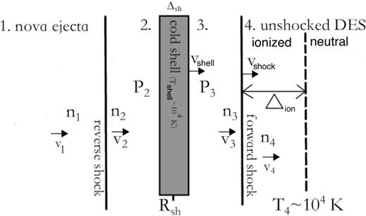
Shock interaction between the fast nova outflow (region 1) and the slower DES (region 4). A forward shock is driven into the DES, while the reverse shock is driven back into the fast ejecta. The shocked ejecta (region 2) and shocked DES (region 3) are separated by a cold central shell containing the swept-up mass. Observed radio emission originates from the forward shock, since emission from the reverse shock is absorbed by the cold central shell. The ionized layer of thickness Δion (equation 5) in front of the forward shock is also shown.
This interaction drives a forward shock through the DES and a reverse shock back through the fast ejecta (see Fig. 2). We assume spherical symmetry and, for the time being, that the shocks are radiative (Section 2.3). For radiative shocks, the post-shock material is compressed and piles up in a central cold shell sandwiched by the ram pressure of the two shocks. Neglecting non-thermal pressure, the shocked gas cools by a factor of ∼103, its volume becoming negligible. Hence, the shocks propagate outwards at the same velocity as the central shell, vshell = vshock ≡ vsh. The velocity of the cold central shell is determined by equating the rate of momentum deposition from ahead and from behind, as described in Paper I.
Evidence for non-thermal radio emission
Fig. 3 shows the radio light curves of three novae with early-time shock signatures: V1324 Sco (Finzell et al. 2015), V1723 Aql (Krauss et al. 2011; Weston et al. 2016b), and V5589 Sgr (Weston et al. 2016a). Thermal free–free emission from the photoionized nova ejecta peaks roughly a year after the outburst (Seaquist & Bode 2008). In V1324 Sco and V1723 Aql, the light curve also shows a second, earlier peak on a characteristic time-scale of a few months. This early peak is also present in V5589 Sgr, although the late thermal peak in this event is only apparent at the highest radio frequencies (Weston et al. 2016a).
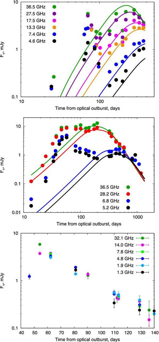
Radio light curves of V1324 Sco (top panel; Finzell et al. 2015), V1723 Aql (middle panel; Krauss et al. 2011; Weston et al. 2016b), and V5589 Sgr (bottom panel; Weston et al. 2016b). In V1723 Aql, only frequencies with full time coverage are shown. In V1324 Sco and V1723 Aql, we show for comparison our best-fitting thermal models (Table 2). In V1324 Sco and V1723 Aql, the maximum uncertainties in the data are 0.3 and 0.1 mJy, respectively, and hence the error bars are not discernible for most of the data points. In V5589 Sgr, we do not attempt to fit a thermal model, even though some of the emission after day 100 could in principle be thermal.
Thermal emission from an expanding sphere is initially characterized by an optically thick, Rayleigh–Jeans spectrum Fν ∝ ν2, with the total flux increasing with the surface area ∝ R2 ∝ t2. Then, starting at high frequencies, the ejecta begins to become optically thin and the radio light curve decays as the radio photosphere recedes back through the ejecta. The shape of the radio light curve near its maximum depends on the density profile of the ejecta, which we take to be that of homologous expansion, n ∝ t−1r−2. Finally, after the entire ejecta becomes optically thin, the spectrum approaches that of optically thin free–free emission, Fν ∝ ν−0.1t−3.
In order to isolate the non-thermal, shock-powered contribution to the radio emission, we first remove the thermal emission from the photoionized ejecta, using a model for the latter as outlined in Bode & Evans (2008). We assume that shocks make no contribution to the emission at late times, t ≳ 100–120 d. Our best-fitting parameters for the ejecta mass of Mej ≈ 2–3 × 10⁻⁴ M⊙ and maximum ejecta velocities of vmax ≈ 1300–1600 km s−1 are compiled in Table 2. Our values are consistent with those found by Weston et al. (2016b) for V1723 Aql. After subtracting the thermal component from the raw fluxes (Fig. 3), the remainder should in principle contain only the shock-powered emission.
Best-fitting parameters for the thermal radio emission models. The fits are based on observations at t ≳ 100–120 d in order to exclude contributions from the early radio peak.
| Nova | D | |$v_{\rm min}^{(a)}$| | |$v_{\rm max}^{(b)}$| | T(c) | |$M_{\rm ej}^{(d)}$| | Δt(e) |
|---|---|---|---|---|---|---|
| (kpc) | (km s−1) | (km s−1) | (K) | (M⊙) | (d) | |
| V1324 Sco | 7.8 | 550 | 1300 | 1.2 × 10⁴ | 2.7 × 10⁻⁴ | 15 |
| V1723 Aq | 6.1 | 270 | 1600 | 1.0 × 10⁴ | 2.2 × 10⁻⁴ | −2.2 |
Notes.(a)Minimum velocity.
(b)Maximum velocity.
(c)Ejecta temperature.
(d)Ejecta mass.
(e)Time delay between outflow ejection and optical outburst.
Our model for the late thermal emission is admittedly simplified, as it assumes a homologous spherically symmetric and isothermal outflow. However, we are primarily interested in modelling the shape of late thermal emission near the time of early radio peak, at around 80–100 d. At this time, the ejecta is still optically thick and thus our only essential assumption is that the outer ejecta is isothermal and expanding ballistically.
Fig. 4 shows the brightness temperature Tb of the early shock-powered radio emission, which we have calculated assuming that the shock-powered emission covers the entire solid angle of the outflow and originates from a radius equal to that of the fastest ejecta inferred from the thermal fit, R = vmaxt. The brightness temperature peaks at values ∼105–106 K which greatly exceed the temperature ∼104 K of the photoionized ejecta inferred at late times (Weston et al. 2016b).
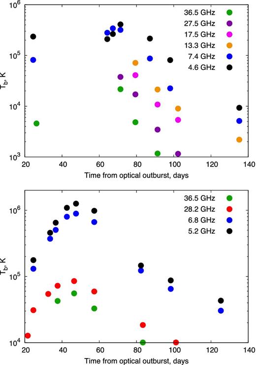
Brightness temperature of the early component of the radio emission for V1324 Sco (top panel) and V1723 Aquila (bottom panel), calculated by subtracting the thermal emission component off the raw fluxes (Fig. 3) and assuming an emitting radius for the non-thermal emission corresponding to the fastest velocity of the ejecta inferred from the thermal fits. In V1723 Aql, only frequencies with full time coverage are shown. In V1324 Sco and V1723 Aql, the maximum uncertainties in the data are 0.3 and 0.1 mJy, respectively, and hence the error bars are not discernible for most of the data points.
Condition for radio maximum
The detection of gamma-rays within days of the optical maximum (Ackermann et al. 2014) demonstrates that shocks are present even early in the nova eruption. However, at such early times, the density of the shocked matter is highest, and radio emission from the shocks is absorbed by the photoionized gas ahead of the shock.
In summary, for characteristic parameters v8 ∼ 0.5–2, ν ∼ 3–30 GHz, the radio light curve peaks when the shock reaches external densities of npk ∼ 106–108 cm−3. These are generally lower than the mean density of the shell at the time of the collision, |$\bar{n}_0$| (equation 2), and those required to produce the observed gamma-ray emission (Metzger et al. 2015). We now consider properties of the forward shock at the radio maximum, defined by n4 = npk.
Is the forward shock radiative or adiabatic?

As we will discuss, in a radiative shock, only the immediate post-shock material contributes to the thermal or non-thermal emission, allowing for faster light-curve evolution. The rapid post-maximum decline of V1324 Sco and V5589 Sgr (tfall ≪ t) is consistent with radiative shocks in these systems (Paper I).
Thermal X-ray emission
Thermal X-rays are diagnostic of the shock velocity and hence of their radiative nature. Fig. 6 shows that the X-ray light curve of V5589 Sgr peaks at a luminosity of LX ∼ 1034 erg s−1 a few weeks after the optical outburst (Weston et al. 2016a). The temperature is very high kT ≳ 30 keV initially, decreasing to ∼1 keV by the radio peak around day 50. Large velocities v8 ≫ 1 are required to produce the high X-ray temperatures at the earliest times, clearly implicating adiabatic shocks. However, the X-ray and radio emission may not originate from the same shocks, while even in a given band different shocks may dominate the emission at different times.
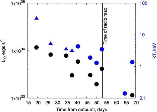
X-ray luminosities (black circles; left axis) and temperature kT (blue circles; right axis) of V5589 Sgr as measured by Swift XRT. Blue triangles indicate temperature lower limits.
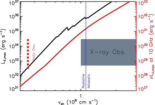
Thermal X-ray luminosity at the time of X-ray peak (black line – left axis; n = nx) and 10 GHz radio luminosity νLν at the time of non-thermal radio peak (red line – right axis; n = npk) as a function of shock velocity. Both luminosities are maximum allowed values, because they are calculated assuming τX = 1 and τν=10 GHz = 1, respectively. We have assumed fiducial parameters for the density scaleheight H = 1014 cm and shock microphysical parameters ϵe = ϵB = 0.01, and a common radius Rsh = 1015 cm and covering fraction fΩ = 1 of the shock. Also shown is the division between radiative and adiabatic shocks (vertical dashed blue line) and the range of observed radio luminosities (dashed red line) and X-ray luminosities and shock velocities corresponding to the observed X-ray temperature (grey region; Table 3, Fig. 6).
For high-velocity shocks (v8 ≳ 1), the predicted X-ray luminosity is several orders of magnitude greater than the observed range in classical novae, LX ∼ 1033–1035 erg s−1 (Mukai & Ishida 2001; Mukai et al. 2008; Osborne 2015; see Table 3). This indicates that the observed X-ray producing shocks either (a) cover a small fraction of the outflow solid angle fΩ ∼ 0.01–0.1 or (b) are produced in regions of the outflow with much lower densities, n ≪ nX, than the mean values |$\bar{n} \sim 10^{7}\hbox{--}10^{9}$| cm−3 (equation 2).
Multiwavelength properties of novae.
| Name | D† | |$L_{\rm 10 GHz,\,pk}^{{\rm nth}}$| | |$L_{\rm 10 GHz,\,pk}^{{\rm th}}$| | LX, pk | |$\frac{L_{\rm 10 GHz, pk}}{L_{\rm X,pk}}$| | |$kT_{\rm pk}^{\ddagger }$| | Lγ, pk | Orientation⨿ |
|---|---|---|---|---|---|---|---|---|
| (kpc) | (erg s−1) | (erg s−1) | (erg s−1) | (keV) | (erg s−1) | |||
| V1324 Sco | 6.5(l)–8(7.8) | 3.4 × 1030(d) | 1.4 × 1030(d) | <1034(h) | >3 × 10⁻⁴ | – | 2.7 × 1036(m) | ? |
| V1723 Aq | 5.3–6.1(6.1)(e) | 2.5 × 1030(d) | 6.3 × 1029(d) | 1.2 × 1034(f) | 2.1 × 10⁻⁴ | 1.8–3(f) | – | I |
| V5589 Sgr | 3.2–4.6(4.0)(b) | 9 × 1029(b) | <3.6 × 1028(b) | 1.2 × 1034(b) | 7.8 × 10⁻⁵ | 0.14–32.7(b) | – | ? |
| V959 Mon | 1.0–1.8(1.4)(a) | <1.1 × 1029(c) | 1.8 × 1029(c) | 2.4 × 1033(g) | <5 × 10⁻⁵ | 3.2(g) | 5.3 · 1034(m) | E |
| V339 Del | 3.9–5.1(4.5)(i) | <2.3 × 1028(k) | 9.2 × 1029(k) | 1.9 × 1033(j) | <1.2 × 10⁻⁴ | >0.8(j) | 2.9 × 1035(m) | F |
Notes.†Estimated uncertainty range of distance, followed in parentheses by the fiducial value adopted in calculating luminosities.
‡Temperature of X-ray emission.
⨿Approximate inclination of binary (E = edge-on; F = face-on; I = intermediate; ? = unknown).
(a) Linford et al. (2015); (b)Weston et al. (2016a); (c)Chomiuk et al. (2014a); (d)Weston et al. (2014); (e)Weston et al. (2016b); (f)Krauss et al. (2011), correct to unabsorbed value; (g)Nelson et al. (2012); (h)for kT ∼ 2–25 keV, Page et al. (2012); (i)Munari et al. (2015); (j)Page & Beardmore (2013); (k)Linford (private communication); (l)Finzell et al. (2015); (m)Ackermann et al. (2014).
The second condition is challenging to satisfy at early times when the densities are probably highest, while both conditions are at odds with the high covering fractions fΩ ∼ 1 and high shock densities needed to power the gamma-ray luminosities (Metzger et al. 2015). We therefore postulate that the hard ≫ keV X-ray emission may not originate from the same shocks responsible for the gamma-ray and non-thermal radio peak, but instead from the low-density polar region (Fig. 1).
In such a scenario, the early radio peak could be powered either by the same fast polar shocks or by lower velocity (v8 ≲ 1) radiative shocks in the higher density equatorial region (Fig. 1). In the latter case, the radio-producing shocks still produce thermal X-rays; however, being comparable in brightness, yet much softer in energy, they may not be readily observable. This would also be true if the X-ray luminosity of radiative shocks is suppressed due to the role of thin-shell instabilities (Kee, Owocki & ud-Doula 2014).
SYNCHROTRON RADIO EMISSION
Leptonic emission
The relativistic leptons responsible for synchrotron radiation originate either from the direct acceleration of electrons via diffusive shock acceleration (DSA; e.g. Blandford & Ostriker 1978) or from electron–positron pairs produced by the decay of charged pions from inelastic proton–proton collisions. Both theory and simulations predict the spectrum of accelerated electrons (dN/dE)dE ∝ E−pdE, with p ≳ 2 (when E ≫ mec2) in the case of strong shocks (Fig. 8, top panel). Two key parameters are the fractions of the shock kinetic power placed into non-thermal electrons and ions, ϵe and ϵp, respectively.

Top panel: energy spectrum of relativistic leptons, calculated for direct shock acceleration of electrons (electron index p = 2) and for secondary pairs from pion decay (proton index p = 2). Bottom panel: synchrotron emissivity as a function of frequency for the particle spectra in the top panel. The thermal free–free emissivity is shown for comparison. Calculations were performed adopting the best-fitting shock parameters for V1324 Sco (Table 4) of v8 = 0.63, ϵe = 0.08, fEUV = 0.05 at the 10 GHz maximum (t = 71.5 d, n4 = 4.5 × 10⁶ g cm−3).
Particle-in-cell (PIC) and hybrid kinetic simulations (e.g. Caprioli & Spitkovsky 2014a,b,c; Kato 2015; Park, Caprioli & Spitkovsky 2015; Wolff & Tautz 2015) indicate that the values of ϵe and ϵp depend on the Mach number of the shock, and the strength and the inclination angle θ of the upstream magnetic field with respect to the shock normal. Shocks which propagate nearly perpendicular to the direction of the magnetic field (θ ≈ 90°) do not efficiently accelerate protons or electrons (Riquelme & Spitkovsky 2011), while those propagating nearly parallel to the magnetic field (θ ≈ 0°) accelerate both (Kato 2015; Park et al. 2015).
What is the geometry of the magnetic field in the ejecta? On time-scales of months, the ejecta has expanded several orders of magnitude from its initial size at the base of the outflow (Metzger et al. 2015). This expansion both dilutes the magnetic field strength via flux freezing and stretches the field geometry to be perpendicular to the radial direction in which the shocks are likely propagating. Based on the above discussion, such a geometry would appear to disfavour hadronic scenarios. However, leptonic scenarios are also strained because the values of ϵe ≳ 10−2 required to explain the gamma-ray emission in V1324 Sco (Metzger et al. 2015) greatly exceed the electron acceleration efficiencies seen in current numerical simulations (Kato 2015; Park et al. 2015).
Due to global asymmetries, or inhomogeneities in the shocked gas caused by radiative instabilities (Metzger et al. 2015), the shocks may not propagate perpendicular to the magnetic field everywhere, allowing hadronic acceleration to operate across a fraction of the shock surface. This possibility motivates considering alternative, hadronic sources for the radio-emitting leptons.
Hadronic emission
Relativistic protons accelerated near the shock collide with thermal protons in the upstream or downstream regions, producing neutral (π0) and charged (π−, π+) pions. The former decay directly into gamma-rays, while π± decay into neutrinos and muons, which in turn decay into relativistic e± pairs and neutrinos. In addition to electrons accelerated directly at the shock, these secondary pairs may contribute to the observed radio emission.
Fig. 8 shows the e± spectrum from pion decay, calculated for a flat input proton energy spectrum (p = 2). Radio emission near the time of peak flux is produced by electrons of energy γpkmec2 ≈ 100 MeV, where γpk ≈ 200 (equation 26). By coincidence, this is close to the pion rest energy mπc2 ≈ 140 MeV and hence to the peak of the e± distribution produced by pion decay. Thus, secondary pairs can contribute significantly to the radio emission if they are deposited in regions where their radiation is observable.
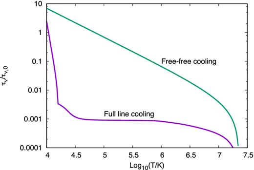
Free–free optical depth τν as a function of gas temperature T behind the shock. The optical depth is normalized to a fiducial value |$\tau _{0,\nu }\equiv (n_{4}/10^{7}{\rm cm^{-3}}) v_8/\nu _{10}^2$|. Different lines correspond to the cases calculated for a cooling function including full line cooling (purple) and one including just free–free cooling (green).
Pairs are also produced by p–p collisions upstream of the shock, which then radiate after being advected into the magnetized downstream. However, proton acceleration via DSA is confined to the narrow photoionized layer ahead of the shock (Metzger et al. 2016), the narrow radial thickness of which, Δion (equation 5), limits the radial extent of the pion production region ahead of the shock.4
RADIO EMISSION MODEL
Pressure evolution of the post-shock gas
Electron and positron spectra
In the hadronic scenario, we model the spectrum of e± pairs from pion decay following Kamae et al. (2006), assuming an input power-law spectrum of relativistic protons Np(E) ∝ E−p with the same energy distribution in the leptonic case.
Radiative transfer equation
Fig. 9 shows the evolution of the optical depth τν/τν, 0 as a function of temperature T behind the shock, where |$\tau _{\nu ,0}=n_{4,7}v_8/\nu _{10}^2$| and τν = 0 is defined at the forward shock surface (T = T3; equation 4). If only free–free cooling is included, then the radio photosphere (τν = 1) can occur at higher temperatures of ≳105 K, depending on τ0,ν. However, if full line cooling is included (Schure et al. 2009), then the photosphere temperature is much lower, ≈104 K. The observed brightness temperatures ≳105 K of nova shocks (Fig. 4) can therefore only be thermal in origin if line cooling is highly suppressed from its standard CIE value (Paper I). When line cooling is present, additional non-thermal synchrotron emission above the photosphere is needed to reproduce the observations.
We assume that the magnetic field does not decay as the plasma cools and compresses downstream of the shock, its strength increasing as B = Bsh(n/n3)Γ, where Γ = 2/3 for the flux freezing of a tangled (statistically isotropic) field geometry. Our results are not sensitive to this choice because, for any physical value of Γ, the integrated emission is dominated by the first cooling length behind the shock (Section 5.1). Using CE ∝ n(p + 2)/3 appropriate for adiabatic compression, the emissivity scales as jν, syn∝n(2p + 3)/3. Fig. 8 compares the frequency dependence of the emissivity for electrons from direct shock acceleration and pion decay.
RESULTS
Analytical estimates
Radiative shocks
Fig. 10 shows how the 10 GHz brightness temperature grows as a function of temperature behind the shock for different assumptions about the cooling and emission of the post-shock gas. At high optical depths, the radiation and gas possess the same temperature (Tν = T) because synchrotron emission is not present in the cold central shell. However, differences in Tν become pronounced as the shock front is approached at T = T3. When line cooling is included, only the first cooling length behind the shock significantly contributes to the final brightness temperature at the shock surface.
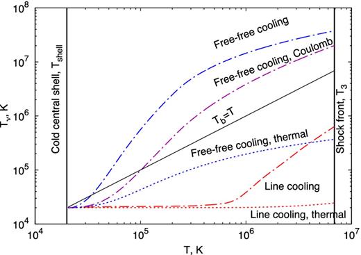
10 GHz brightness temperature in the post-shock region as a function of gas temperature T < T3 behind the shock (T = T3). Different lines correspond to different assumptions about (1) whether the emission accounts only for thermal free–free emission (dashed lines) or also includes non-thermal synchrotron emission (dash–dotted lines), and (2) whether the assumed cooling function is just free–free emission (blue, purple) or also includes emission lines (red). A purple line shows the non-thermal case with free–free cooling, including the effect of Coulomb losses on the emitting relativistic leptons. All calculations were performed for a pre-shock density of n4 = 4.5 × 10⁶ g cm−3 corresponding to the 10 GHz peak time, adopting the best-fitting shock parameters for V1324 Sco (Table 4) of v8 = 0.63, ϵe = 0.08, fEUV = 0.05.
Coulomb losses of relativistic electrons only noticeably impact the non-thermal emission well downstream of the shock, in regions where the gas temperature is ≲105 K (equation A2). Coulomb losses therefore significantly impact the observed radiation temperature only if free–free cooling dominates, for which contributions to the emission from the post-shock gas Tν ∝ T1/6 (equation 40) vary only weakly with gas temperature. Even in this case, however, the observed temperature reduced only by a factor of ∼2 compared to an otherwise identical case neglecting Coulomb losses. Coulomb corrections are completely negligible in our fiducial models when line cooling is included because the bulk of the emission comes from immediately behind the shock, where the temperature is high and the density is low.
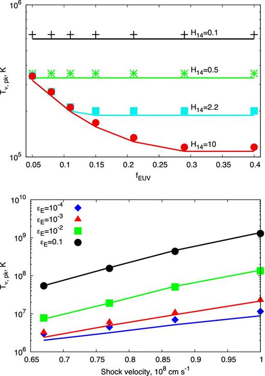
Peak brightness temperature of non-thermal emission as a function of shock parameters. The top panel shows |$T_{\nu \rm , pk}^{\rm nth}$| as a function of the fraction of shock energy used for ionization fEUV and density scaleheight H. The bottom panel shows |$T_{\nu \rm , pk}^{\rm nth}$| as a function of the shock velocity, v8, and fraction of the shock energy placed into relativistic electrons, ϵe. Results of the full calculation are shown as symbols, while the analytic estimates from equation (40) are shown as lines. The values of parameters not varied in these figures are taken as best-fitting values for V1324 Sco (Table 4).

The top panel of Fig. 11 shows how |$T_{\nu , \rm pk}^{\rm nth}$| depends on the density scaleheight H and the ionized fraction of the pre-shock layer, fEUV. When the value of H is small, or fEUV is sufficiently high, then the entire DES scaleheight is ionized (H = Δion) and the peak brightness temperature is independent of fEUV. On the other hand, when Δion < H, then the brightness temperature is independent of H but decreases with increasing ionizing radiation as |$T_{\rm \nu ,pk}^{\rm nth}\propto f_{\rm EUV}^{-(p+1)/4}\underset{p=2}{=}f_{\rm EUV}^{-0.75}$| (equation 43). The bottom panel of Fig. 11 shows how the peak temperature depends on the shock velocity, |$\tilde{v}_{\rm f}$|, and the electron acceleration efficiency, ϵe.
Fig. 12 compares the brightness temperature calculated in a purely thermal model (ϵe = 0) to our analytic estimate of |$T_{\nu , \rm pk}^{\rm th}$| (equation 42). For a broad range of parameters, the peak temperatures fail to exceed 105 K, making thermal models of radiative shocks challenging to reconcile with observations (see Fig. 4).
Adiabatic shocks
For higher velocity v8 ≳ 108 cm s−1, adiabatic shocks, the brightness temperature is again estimated by assuming that the first scaleheight H behind the shock dominates the emission, i.e. neglecting ongoing emission from matter shocked many dynamical times earlier. However, unlike with radiative shocks, this assumption cannot be rigorously justified without a radiation hydrodynamical simulation, an undertaking beyond the scope of this paper.
For adiabatic shocks, the peak thermal brightness temperature is a decreasing function of the shock velocity due to the αff ∝ T−3/2 dependence of free–free absorption. Comparing equations (44) and (46), a maximum thermal brightness temperature of ≈104 K is thus obtained for the intermediate shock velocity v8 ∼ 1 separating radiative from adiabatic shocks. The fact that this falls well short of observed peak brightness temperatures (Fig. 4) again disfavours thermal models for the early radio peak.
Radio light curves and spectra
The shape of the radio light curve and spectrum are driven by the effects of free–free opacity, which are independent of the emission mechanism and hence apply both to thermal (Paper I) and non-thermal models. Fig. 13 shows an example model light curve (upper panel) and corresponding evolution of the spectral index across two representative frequency ranges (bottom panel). At high frequencies, the light curve peaks earlier and reaches a larger maximum flux, due to the frequency dependence of free–free absorption, αff ∝ ν−2, and the monotonically declining shock power. When such behaviour is not observed, this indicates that our one-zone model is inadequate or that free–free opacity does not determine the light-curve maximum (Section 6.3).
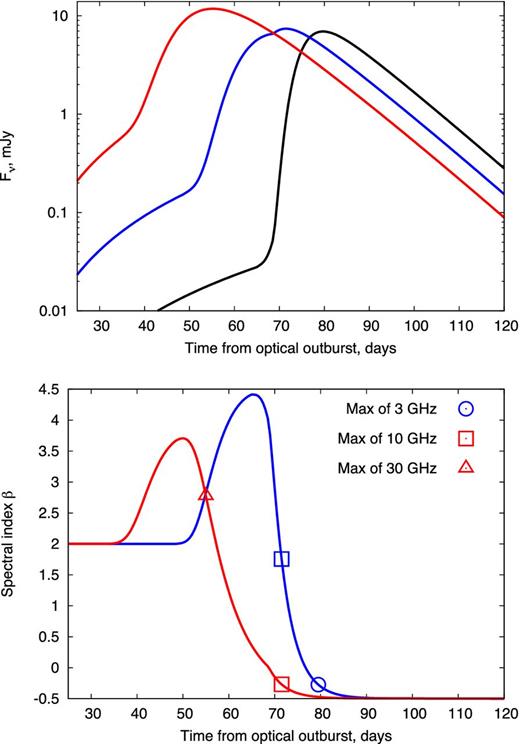
Top: example model radio light curves at radio frequencies of 3 GHz (black), 10 GHz (blue), and 30 GHz (red), calculated for our best-fitting parameters for V1324 Sco (Table 4). The light curve does not include thermal emission from the cold central shell or other sources of photoionized ejecta. Bottom: measured spectral index β between the 3 and 10 GHz bands (red) and the 10 and 30 GHz bands (blue). The times of light-curve maxima are marked with symbols for 3 GHz (circle), 10 GHz (square), and 30 GHz (triangle). The plateau at β = 2 at early times corresponds to when the photoionized layer ahead of the shock is still optically thick.
The spectral index β initially rises to exceed that of optically thick isothermal gas (β > 2) because the higher frequency emission peaks first. Then, once the lower frequency emission peaks, the shock becomes optically thin and hence the spectral index approaches the spectral index of optically thin synchrotron emission. Importantly, a flat spectral index does not itself provide conclusive evidence for non-thermal synchrotron emission, even though the optically thin spectral indices are different for synchrotron and thermal bremsstrahlung emission. The emission mechanism is instead more accurately distinguished from thermal emission based on the higher peak brightness temperatures which can be achieved by non-thermal models. Also, at late times, the radio emission should eventually come to be dominated by thermal emission of the photoionized ejecta and hence the spectral index will again rise to β = 2. This feature is not captured by Fig. 13 because we have not included thermal emission from the cool central shell or other sources of photoionized ejecta.
Fits to individual novae
We fit our model to the radio light curves of three novae with early-time coverage, V1324 Sco, V1723 Aql, and V5589 Sgr (Figs 3 and 4). We employ a χ-squared minimization technique across nine free parameters: v1, v4, n4/n1, Δt, H, n0, p, ϵe, fEUV. We assume a shock covering fraction of fΩ = 1 and take ϵB = 0.01, as the latter is degenerate with ϵe. Table 4 provides the best-fitting parameters of each nova. Although the electron power-law index is a free parameter, in practice it always converges to a best-fitting value of p ≃ 2.
Best-fitting parameters of synchrotron model.
| Nova | |$v_1^{(a)}$| | |$v_4^{(b)}$| | |$n_{4}/n_{1}^{(c)}$| | |$\tilde{v}_{\rm f}^{(d)}$| | Δt(e) | H(f) | n0(g) | ϵe(h) | fEUV(i) |
|---|---|---|---|---|---|---|---|---|---|
| (km s−1) | (km s−1) | (km s−1) | (d) | (cm) | (cm−3) | ||||
| V1324 Sco | 1700 | 670 | 0.43 | 630 | 12 | 3.7 × 10¹³ | 7.8 × 10⁹ | 0.081 | 0.051 |
| V1723 Aql | 2300 | 770 | 0.66 | 830 | 3.2 | 9.5 × 10¹³ | 6.7 × 10⁷ | 0.015 | 0.31 |
| V5589 Sgr | 2200 | 190 | 2.3 | 810 | 5 | 6.8 × 10¹³ | 4.1 × 10⁸ | 0.014 | 0.07 |
Notes.(a)Velocity of fast outflow.
(b)Velocity of slow outflow (DES).
(c)Ratio of densities of DES and fast outflow.
(d)Velocity of the shock in the frame of the upstream gas, calculated from v1, v4, n4/n1 using equation (3).
(e)Time delay between launching fast and slow outflows.
(f)Scaleheight of slow outflow.
(g)Normalization of density profile of slow outflow (equation 7).
(h)Fraction of shock power placed into power-law relativistic electrons/positrons.
(i)Fraction of shock power placed into hydrogen-ionizing radiation (equation 5).
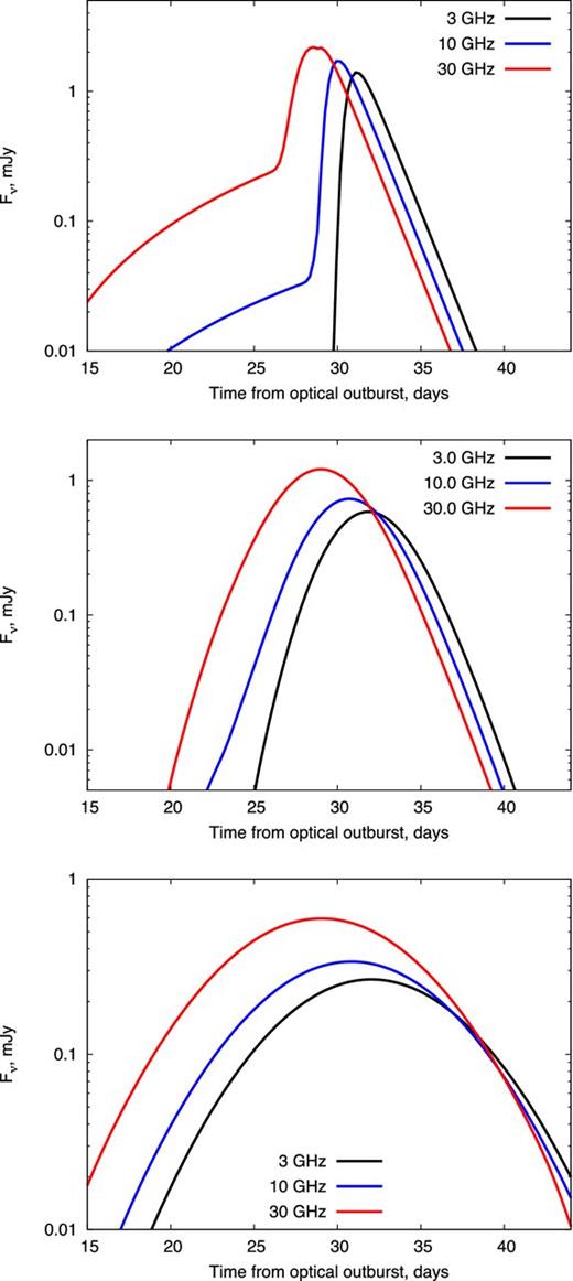
Our best fit to V1324 Sco is shown in the upper panel of Fig. 14. The best-fitting shock velocity of 640 km s−1 is within the range of radiative shocks, consistent with the rapid post-maximum decline. For the parameters of our best-fitting model, npk,Δ/npk,H = 0.96ν10, implying that for frequencies above (below) 10 GHz the thickness of ionization layer is less than (greater than) the scaleheight at the time of peak flux. The transition between these two regimes can be seen as a small break in the 7.4 GHz light curve around day 68. Substituting our best-fitting parameters into equation (1), we find that the collision occurred 20 d after the start of the outflow, corresponding to 7 d after the onset of the gamma-ray emission (Ackermann et al. 2014). This discrepancy is not necessarily worrisome, as the colliding ‘shells’ may be ejected over days or longer.

V1723 Aql was more challenging to fit (Fig. 14, middle panel), mainly because different frequencies peak at nearly the same time. This is contrary to the expectation that high frequencies will peak first if free–free absorption indeed controls the light-curve rise, as our model assumes (see Section 6.3 for alternative interpretations). Although we cannot fit V1723 Aql in detail, we can nevertheless reproduce the magnitudes of the peak fluxes for reasonable parameters. Our best-fitting model for V5589 Sgr is shown in the bottom panel of Fig. 14, although the data are more sparse than for the other two events.
DISCUSSION
Efficiency of relativistic particle acceleration
Such high acceleration efficiencies disfavour hadronic scenarios for the radio-emitting leptons, which are estimated to produce ϵe ≲ 10−4 (equation 27). They are also in tension with PIC simulations of particle acceleration at non-relativistic shocks (Kato 2015; Park et al. 2015) which find ϵe ∼ 10−4 when extrapolated to shock velocities v8 ≲ 103 km s−1, modelling of supernova remnants (Morlino & Caprioli 2012, ϵe ∼ 10−4), and Galactic cosmic ray emission (Strong et al. 2010, ϵe ∼ 10−3). On the other hand, the inferred cosmic ray efficiencies are dependent on the shock fraction of the accelerated electrons which escape the supernova remnant. Modelling of unresolved younger radio supernovae typically finds higher values of ϵe (Chevalier 1982; Chandra et al. 2012), consistent with our results. Given these observational and theoretical uncertainties, we tentatively favour a leptonic source for the radio-emitting electrons.
In the above, we have assumed that the shocks cover a large fraction of the outflow surface (fΩ ∼ 1). However, if instead we have fΩ ≪ 1, then the required values of ϵe and ϵB would be even higher than their already strained values. If the radio-emitting shocks are radiative, they must therefore possess a large covering fraction fΩ ∼ 1.
Lower values of ϵe and ϵB are allowed if the radio emission is instead dominated by high-velocity v8 ≳ 1, adiabatic shocks covering a large solid fraction fΩ ∼ 1. The sensitive dependence of the brightness temperature on the shock velocity implies that even a moderate increase in |$\tilde{v}_{\rm f}$| can increase the radio flux by orders of magnitude for fixed ϵe, ϵB. On the other hand, the adiabatic shocks responsible for the hard X-rays appear to require a small covering fraction fΩ ≪ 1 so as not to overproduce the observed X-ray luminosities (Section 2.4).
The DES is not an MS progenitor wind
Radio emission from the interaction of the nova ejecta with the MS progenitor wind is thus undetectable for physical values of |$\dot{M}$|, unless the mass-loss rate is comparable to that of the nova eruption itself.
Light curve of V1723 Aquila
Our model does not provide a satisfactory fit to the light curve of V1723 Aql because all radio frequencies peak nearly simultaneously (Fig. 14), contrary to the expectation if the light curve peaks due to the decreasing free–free optical depth (Section 5.3). Here we describe modifications to the standard picture that could potentially account for this behaviour.
Steep density gradient
Fig. 15 shows the light curves of our single-zone model (for an assumed scaleheight of H = 5 × 1012 cm) convolved with a Gaussian profile of different widths σ, in order to crudely mimic the effects of non-simultaneous shock emergence. The top panel shows the unaltered radio light curve, i.e. assuming simultaneous shock emergence, which again makes clear that the high frequencies peak first (Section 2.2). The middle and bottom panels show the same light curve, but smeared over time intervals of σ = 2 and 5 d, respectively. In this way, the difference between the times of maximum at different frequencies can be substantially smaller than the rise or fall time, as observed in V1723 Aql.
Example light curves (with late-time thermal emission subtracted) for a steep density gradient H = 5 × 1012 cm, which has been convolved with a Gaussian of different widths σ = 0 (top panel), σ = 2 d (middle panel), and σ = 5 d (bottom panel). This illustrates how a shock propagating down a steep density profile, but reaching the DES surface at different times at different locations across the ejecta surface, can produce the appearance of an achromatic light curve.
Collision with optically thin shell
Another possibility is that the radio-producing shock occurs in a dilute thin shell, which has a lower density than the mean density of the DES, i.e. n0 ≪ npk ∼ 107 cm−1. Absorption then plays no part in the light-curve rise, which is instead controlled by the time required for the shock to cross the radial width of the shell.
Although the parameter space for an optically thin shell (τsh < 0.1) which is radiative (η ≲ 1) is not large, this represents a viable explanation for the behaviour of V1723 Aquila.
Radio emission from polar adiabatic shocks
Fig. 7 shows the maximum X-ray luminosity and the maximum 10 GHz radio luminosity as a function of the shock velocity, spanning the range from radiative (v8 ≲ 1) to adiabatic (v8 ≳ 1) shocks. Both radio and X-ray luminosities increase by many orders of magnitude across this range. However, their ratioLR/LX coincidentally varies only weakly with v8, as shown in Fig. 16. Absolute luminosities depend on the covering fraction and radius of the shock, but this ratio is obviously independent of these uncertain quantities. Reasonable variations in the density scaleheight H, ionization fraction fEUV, and the CNO abundances result in a factor of ≲3 variation in this ratio (Fig. 16, top panel), which is instead most sensitive to the microphysical parameters, |$\propto \epsilon _{\rm e} \epsilon _B^{3/4}$| for p = 2 (Fig. 16, bottom panel). Any shock producing X-rays will therefore also produce radio emission of intensity comparable to the observed values. Fig. 16 shows for comparison the measured value of LR/LX, or limits on its value, using the observed peak X-ray and non-thermal radio luminosities for five novae.
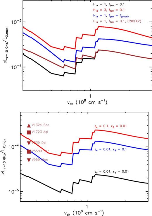
Ratio of non-thermal peak 10 GHz radio luminosity (equation 44) to peak thermal X-ray luminosity (equation 19) as a function of shock velocity vsh. The X-ray luminosity is calculated for the pre-shock density n4 = nX (equation 22), the latter calculated using the bound–free cross-sections from Verner et al. (1996) for our assumed ejecta composition. The top panel shows that the ratio of luminosities varies by only a factor of a few for realistic variations in the density scaleheight H, the ionized fraction fEUV, or if the CNO mass fraction is doubled. The bottom panel shows the more sensitive dependence of the luminosity ratio on the shock microphysical parameters ϵe and ϵB, calculated for H14 = 1, fEUV = 0.1, and standard CNO abundances. Shown for comparison are measurements (squares), or limits (triangles) on the luminosity ratio of the novae compiled in Table 3.
The early-time X-rays in some novae are too hard to originate from radiative shocks (Table 3, Fig. 6) and thus could instead originate from fast adiabatic shocks in the low-density polar regions (Fig. 1; Section 2.4). If all the observed X-rays originate from fast polar shocks, and all radio emission from slower equatorial radiative shocks, then the measured ratio LR/LX = LR, rad/LX + LR, ad/LX, comprised of contributions from both radiative and adiabatic shocks, should exceed the ratio shown in Fig. 16. For V1324 Sco, V1723 Aql, and V5589 Sgr, this requires that |$\epsilon _{\rm e} \epsilon _B^{3/4} \approx 10^{-3}$|, consistent with our best-fitting values found earlier. The non-detections of non-thermal radio emission in V339 Del and V959 Mon also do not contradict |$\epsilon _{\rm e} \epsilon _B^{3/4} \approx 10^{-3}$|. We conclude that, within the uncertainties, the thermal X-ray and non-thermal radio emission in novae is consistent with originating from distinct shocks.
CONCLUSIONS
We have explored non-thermal synchrotron radio emission from radiative shocks as a model for the early radio peaks in novae by means of a one-dimensional model. Broadly speaking, we find that the measured brightness temperatures can be explained for physically reasonable parameters of the shock velocity and microphysical parameters ϵe and ϵB (Table 4). The presence of a detectable early radio peak requires the presence of DES of density ≳106–107 cm−3 on a radial scale of ≈1014–1015 cm from the white dwarf. The emission from the nova ejecta colliding with a progenitor wind of mass-loss rate |$\dot{M}\lesssim 10^{-9}\,{\rm M}_{\odot }$| yr−1 is not sufficient to explain the observed radio peaks (Section 6.2).
The thin photoionized layer ahead of the forward shock plays a key role in our model, as its free–free optical depth determines the time, intensity, and spectral indices near the peak of the emission (see Section 2.2). One-dimensional models robustly predict that higher frequency emission peaks at earlier times, imprinting a distinct evolution on the spectral index (Fig. 13) which is independent of whether the emission mechanism is thermal or non-thermal. V1324 Sco and V5589 Sgr do exhibit this behaviour, but in V1723 Aql the light curves at all frequencies peak at nearly the same time. Possible explanations include the nova outflow colliding with a shell of much lower density than the mean density of the nova ejecta (Section 6.3). Alternatively, the evolution may appear achromatic if the shock breaks out of the DES at different times across different parts of its surface, as would occur if the DES is not spherically symmetric (Fig. 15).
Because the light-curve evolution is controlled by free–free opacity effects, one cannot readily distinguish thermal from non-thermal emission based on the spectral index evolution alone. Thermal emission models exhibit spectral index behaviour (Paper I) which is very similar to the non-thermal model described here (Fig. 13). Non-thermal emission is best distinguished by the much higher brightness temperatures which can be achieved than for thermal emission.
The relativistic electrons (or positrons) responsible for the non-thermal synchrotron emission originate either from direct diffusive acceleration at the shock (leptonic scenario) or as secondary products from the decays of pions produced in proton–proton collisions (hadronic scenario). In either case, the radio-emitting leptons are identical, or tightly related, to the particles which power the observed γ-ray emission. For instance, if the observed ≳100 MeV gamma-rays are produced by relativistic bremsstrahlung emission (as favoured in leptonic scenario by Metzger et al. 2015), then the energies of the radiating electrons (also ≳100 MeV) are very close to those which determine the peak of the radio synchrotron emission at later times (equation 26). Likewise, gamma-rays from π0 decay in hadronic scenarios are accompanied by electron/positron pairs with energies ≳100 MeV in the same range, as determined by the pion rest mass. Once produced, relativistic leptons evolve approximately adiabatically downstream of the shock for conditions which characterize the radio maximum. The only possible exception is Coulomb cooling in the cases when free–free emission dominates lines in cooling the post-shock thermal gas (Fig. 10).
In hadronic scenarios, only a small fraction of relativistic protons produce pions in the downstream before being advected into the central cold shell (from which radio emission is heavily attenuated by free–free absorption). Relativistic protons therefore provide considerable pressure support in the post-shock cooling layer, preventing the gas from compressing by more than an order of magnitude (Section 4.1). The possible role of clumping due to thermal instability of the radiative shock on this non-thermal pressure support deserves further attention, as the central shell may provide a shielded environment which is conducive to dust and molecule formation in novae (Derdzinski et al., in preparation).
The small number of pions produced in the rapidly cooling post-shock layer implies that of the ≲10 per cent of the total shock power placed into relativistic protons, only a tiny fraction ϵe ∼ 10−4 (equation 27) goes into e± pairs capable of producing detectable radio emission. For physical values of ϵB ≲ 0.1, the critical product |$\epsilon _{\rm e}\epsilon _B^{3/4} \lesssim 10^{-5}$| which controls the brightness temperature is a few orders of magnitude below that required by data of ∼10−4–10−3 (equations 51–53). We therefore disfavour the hadronic scenario for radio-producing leptons. This does not rule out a hadronic origin for the γ-ray emission, but it does suggest that the direct acceleration of electrons is occurring at the gamma-ray producing shocks.
Within leptonic scenarios, the values of |$\epsilon _{\rm e} \epsilon _B^{3/4}$| required by the radio data are typically higher than those measured from PIC simulations (Caprioli & Spitkovsky 2014a) and by modelling Galactic supernova remnants (Morlino & Caprioli 2012). However, values of |$\epsilon _{\rm e} \epsilon _B^{3/4}\sim 10^{-4}\hbox{--}10^{-3}$| do appear similar to those inferred by modelling young radio supernovae (e.g. Chandra et al. 2012).
We confirm the finding of Paper I that when CIE line cooling is included, thermal emission from radiative shocks cannot explain the early high brightness temperature radio peak. Perhaps the best evidence for non-thermal radio emission comes from the cases like V1324 Sco, where no X-ray emission is detected. An X-ray non-detection implies a low-velocity, radiative shock, which would be especially challenged to produce a significant radio flux in the early peak without a non-thermal contribution. We can also rule out thermal emission from an adiabatic shock, at least under the assumption that only the first scaleheight behind the shock dominates that contributing to the observed emission (Section 6.4). Future radiation hydrodynamical simulations of adiabatic shocks and their radio emission in the case of a steep density gradient are needed to determine whether thermal adiabatic shocks can be completely ruled out.
We have derived analytic expressions for the peak brightness temperature of non-thermal synchrotron emission (equation 44). Our model can reproduce the observed fluxes of V5589 Sgr, V1723 Aql, and V1324 Sco and, in the case of V1324 Sco, details of the radio light curve. Non-detections of early radio peak from V959 Mon and V339 Del place upper limits on ϵe, ϵB. The upper limits for V339 Del and V959 Mon are broadly consistent with the inferred values of ϵe, ϵB values for novae with detected early radio peak.
In summary, radio observations of novae provide an important tool for studying particle acceleration and magnetic field amplification in shocks which is complementary to γ-rays observations. They also inform our understanding of the structure of the nova ejecta and internal shocks, which may vary considerably with time and as a function of polar angle relative to the binary axis.
We thank Laura Chomiuk, Tom Finzell, Yuri Levin, Koji Mukai, Michael Rupen, Jeno Sokoloski, and Jennifer Weston for helpful conversations. We also thank Jeno Sokoloski for providing us with the numerical tools to fit the thermal radio emission. ADV and BDM gratefully acknowledge support from NASA grants NNX15AU77G (Fermi), NNX15AR47G (Swift), and NNX16AB30G (ATP), and NSF grant AST-1410950, and the Alfred P. Sloan Foundation.
Ionizing X-rays from the white dwarf are likely blocked by the neutral central shell in the equatorial plane, although they may escape along the low-density polar region (Fig. 1). Many novae are not detected as supersoft X-ray sources until after the early shock-powered radio emission has peaked (Schwarz et al. 2011).
Note that η also equals the ratio of the post-shock cooling length
The ‘Razin’ effect suppresses synchrotron radiation below a critical frequency νR = νpγ (Rybicki & Lightman 1979), where νp = (npke2/πme)1/2. For γ = γpk, we thus have |$\nu /\nu _{\rm R}= 4.5 \, \epsilon _{B,-2}^{1/4}v_8^{5/4}f_{\rm EUV,-1}^{1/4}$|. Since for parameters of interest we have ν ≳ νR, modifications from the Razin effect should be weak and are hereafter neglected.
Very high energy protons of energy ∼Emax ≳ 10 GeV leak out of the DSA cycle, escaping into the neutral upstream with a nearly mono-energetic distribution with a comparable energy flux to the power-law spectrum ultimately advected downstream (e.g. Caprioli & Spitkovsky 2014a). However, the upstream-stream protons inject pairs at multi-GeV energies ≫γpkmec2 (equation 26) which radiate most of their synchrotron emission at higher frequencies than that responsible for the bulk of the radio emission.
Soft X-rays are in the Thomson regime for interacting with γ ∼ 100 electrons.
REFERENCES
APPENDIX: NON-THERMAL ELECTRON COOLING IN THE POST-SHOCK COOLING LAYER
In calculating the radio synchrotron emission from nova shocks, we assume that relativistic electrons and e± pairs evolve adiabatically in the post-shock cooling layer. This assumption is justified here by comparing various sources of cooling (Coulomb, bremsstrahlung, inverse Compton) to that of the background thermal plasma, tcool (equation 14). We again focus on electrons or positrons with Lorentz factors of γpk ∼ 200 (equation 26), as these determine the synchrotron flux near the light-curve peak, where n3 = 4n4 = 4npk.
In summary, relativistic radio-emitting leptons cool in the post-shock gas on a time-scale which is generally much longer than that of the thermal background plasma for the range of velocities v8 ≲ 1 of radiative shocks. This justifies evolving their energies adiabatically behind the shock, with the possible exception of Coulomb losses, which are unimportant immediately behind the shock but may become so as gas compresses to higher densities n ≫ n3.
