


Abstract
We present results from a joint XMM–Newton/NuSTAR monitoring of the Seyfert 1 NGC 4593, consisting of 5 × 20 ks simultaneous observations spaced by 2 d, performed in 2015 January. The source is variable, both in flux and spectral shape, on time-scales down to a few ks and with a clear softer-when-brighter behaviour. In agreement with past observations, we find the presence of a warm absorber well described by a two-phase ionized outflow. The source exhibits a cold, narrow and constant Fe Kα line at 6.4 keV, and a broad component is also detected. The broad-band (0.3–79 keV) spectrum is well described by a primary power law with Γ ≃ 1.6–1.8 and an exponential cut-off varying from |$90^{+ 40}_{- 20}$| to >700 keV, two distinct reflection components, and a variable soft excess correlated with the primary power law. This campaign shows that probing the variability of Seyfert 1 galaxies on different time-scales is of prime importance to investigate the high-energy emission of active galactic nuclei.
INTRODUCTION
Active galactic nuclei (AGN) are thought to be powered by an accretion disc around a supermassive black hole, mostly emitting in the optical/ultraviolet (UV) band. According to the standard paradigm, the X-ray emission is due to thermal Comptonization of the soft disc photons in a hot region, the so-called corona (Haardt & Maraschi 1991; Haardt, Maraschi & Ghisellini 1994, 1997). This process explains the power-law shape of the observed X-ray spectrum of AGN. A feature of thermal Comptonization is a high-energy cut-off, which has been observed around ∼100 keV in several sources thanks to past observations with Compton Gamma-Ray Observatory (CGRO)/Oriented Scintillation Spectrometer Experiment (OSSE; Zdziarski, Poutanen & Johnson 2000), BeppoSAX (Perola et al. 2002) and more recently Swift/Burst Alert Telescope (BAT; Baumgartner et al. 2013) and INTEGRAL (Malizia et al. 2014; Lubiński et al. 2016). From the application of Comptonization models, such high-energy data allow to constrain the plasma temperature, which is commonly found to range from 50 to 100 keV (e.g. Zdziarski et al. 2000; Lubiński et al. 2016). Furthermore, the cut-off energy is now well constrained in an increasing number of sources thanks to the unprecedented sensitivity of NuSTAR up to ∼80 keV (e.g. Ballantyne et al. 2014; Brenneman et al. 2014; Marinucci et al. 2014; Baloković et al. 2015; Matt et al. 2015; Ursini et al. 2015). The primary X-ray emission can be modified by different processes, such as absorption from neutral or ionized gas (the so-called warm absorber), and Compton reflection from the disc (e.g. George & Fabian 1991; Matt, Perola & Piro 1991) or from more distant material, like the molecular torus at pc scales (e.g. Matt, Guainazzi & Maiolino 2003). A smooth rise below 1–2 keV above the extrapolated high-energy power law is commonly observed in the spectra of AGN (see e.g. Bianchi et al. 2009). The origin of this so-called soft excess is uncertain (see e.g. Done et al. 2012). Ionized reflection is able to explain the soft excess in some sources (e.g. Crummy et al. 2006; Ponti et al. 2006; Walton et al. 2013), while Comptonization in a ‘warm’ region is favoured in other cases (e.g. Mehdipour et al. 2011; Boissay et al. 2014).
The current knowledge of the geometrical and physical properties of the X-ray corona is far from being complete, as in most sources we still lack good constraints on the coronal temperature, optical depth and geometry. The approach based on multiple, broad-band observations with a high signal-to-noise ratio is a powerful tool to study the high-energy emission in Seyfert galaxies. Strong and fast X-ray variability, both in flux and spectral shape, is a hallmark of AGN, and of historical importance to rule out alternatives to supermassive black holes as their central engine (e.g. Elliot & Shapiro 1974). The analysis of X-ray variability allows disentangling the different spectral components and constraining their characteristic parameters, as shown by recent campaigns on Mrk 509 (Kaastra et al. 2011; Petrucci et al. 2013) and NGC 5548 (Kaastra et al. 2014; Ursini et al. 2015).
In this paper, we discuss results based on a joint XMM–Newton and NuSTAR monitoring program on NGC 4593 (z = 0.009; Strauss et al. 1992), an X-ray bright Seyfert 1 galaxy hosting a supermassive black hole of (9.8 ± 2.1) × 106 solar masses (from reverberation mapping; see Denney et al. 2006). This is the first monitoring carried out by XMM–Newton and NuSTAR specifically designed to study the high-energy emission of an AGN through the analysis of its variability on time-scales of days. We reported preliminary results from a phenomenological timing analysis in Ursini et al. (2016). Here we focus on the broad-band (0.3–80 keV) X-ray spectral analysis. Past observations of NGC 4593 with BeppoSAX (Guainazzi et al. 1999), XMM–Newton (Reynolds et al. 2004; Brenneman et al. 2007) and Suzaku (Markowitz & Reeves 2009) have shown a strong reflection bump above 10 keV and the presence of two narrow Fe Kα emission lines at 6.4 and around 7 keV. A soft excess below 2 keV has been reported, both in the 2002 XMM–Newton data (Brenneman et al. 2007) and in the 2007 Suzaku data, with a drop in the 0.4–2 keV flux by a factor of >20 in the latter (Markowitz & Reeves 2009). Guainazzi et al. (1999) found a lower limit on the high-energy cut-off of 150 keV from BeppoSAX data.
This paper is organized as follows. In Section 2, we describe the observations and data reduction. In Section 3 we present the analysis of the XMM–Newton and NuSTAR spectra. In Section 4, we discuss the results and summarize our conclusions.
OBSERVATIONS AND DATA REDUCTION
XMM–Newton (Jansen et al. 2001) and NuSTAR (Harrison et al. 2013) simultaneously observed NGC 4593 five times, spaced by 2 d, between 2014 December 29 and 2015 January 6. Each pointing had an exposure of ∼20 ks. We report in Table 1 the log of the data sets.
The logs of the joint XMM–Newton and NuSTAR observations of NGC 4593.
| Obs. | Satellites | Obs. Id. | Start time (utc) | Net exp. |
|---|---|---|---|---|
| yyyy-mm-dd | (ks) | |||
| 1 | XMM–Newton | 0740920201 | 2014-12-29 | 16 |
| NuSTAR | 60001149002 | 22 | ||
| 2 | XMM–Newton | 0740920301 | 2014-12-31 | 17 |
| NuSTAR | 60001149004 | 22 | ||
| 3 | XMM–Newton | 0740920401 | 2015-01-02 | 17 |
| NuSTAR | 60001149006 | 21 | ||
| 4 | XMM–Newton | 0740920501 | 2015-01-04 | 15 |
| NuSTAR | 60001149008 | 23 | ||
| 5 | XMM–Newton | 0740920601 | 2015-01-06 | 21 |
| NuSTAR | 60001149010 | 21 |
XMM–Newton observed the source using the European Photon Imaging Camera (EPIC; Strüder et al. 2001; Turner et al. 2001) and the Reflection Grating Spectrometer (RGS; den Herder et al. 2001). The EPIC instruments were operating in the Small Window mode, with the medium filter applied. Because of the significantly lower effective area of the MOS detectors, we only report the results obtained from pn data. The data were processed using the XMM–Newton Science Analysis System (sas v14). Source extraction radii and screening for high-background intervals were determined through an iterative process that maximizes the signal-to-noise ratio (Piconcelli et al. 2004). The background was extracted from circular regions with a radius of 50 arcsec, while the source extraction radii were in the range 20–40 arcsec. The EPIC-pn spectra were grouped such that each spectral bin contains at least 30 counts, and not to oversample the spectral resolution by a factor greater than 3. The RGS data were extracted using the standard sas task rgsproc.
The NuSTAR data were reduced using the standard pipeline (nupipeline) in the NuSTAR Data Analysis Software (nustardas, v1.3.1; part of the heasoft distribution as of version 6.14), using calibration files from NuSTARcaldb v20150316. Spectra and light curves were extracted using the standard tool nuproducts for each of the two hard X-ray detectors aboard NuSTAR, which sit inside the corresponding focal plane modules A and B (FPMA and FPMB). The source data were extracted from circular regions with a radius of 75 arcsec, and background was extracted from a blank area with the same radius, close to the source. The spectra were binned to have a signal-to-noise ratio greater than 5 in each spectral channel, and not to oversample the instrumental resolution by a factor greater than 2.5. The spectra from FPMA and FPMB were analysed jointly but not combined.
In Fig. 1 we show the light curves in different energy ranges of the five XMM–Newton and NuSTAR observations. The light curves exhibit a strong flux variability, up to a factor of ∼2, on time-scales as short as a few ks. In Fig. 1 we also show the XMM–Newton/pn (2–10 keV)/(0.5–2 keV) hardness ratio light curve and the NuSTAR (10–50 keV)/(3–10 keV) hardness ratio light curve. These light curves show a significant spectral variability, particularly in the softer band, with a less prominent variability in the harder band. From these plots, it can be seen that a higher flux is associated with a lower hardness ratio, i.e. we observe a ‘softer when brighter’ behaviour (see also Ursini et al. 2016). During the first observation, both flux and spectral variability are particularly strong. To investigate the nature of these variations, we analysed the spectra of each observation separately, splitting only the first observation into two ∼10 ks long bits (see Fig. 1). We did not split the time intervals for the extraction of the spectra further, because in the other observations the spectral variability is less pronounced. This choice leaves us with a total of six spectra from our campaign, which we analyse in the following.

The light curves of the five joint XMM–Newton and NuSTAR observations of NGC 4593. Time bins of 1 ks are used. Top panel: the XMM–Newton/pn count rate light curve in the 0.5–2 keV band. Second panel: the XMM–Newton/pn count rate light curve in the 2–10 keV band. Third panel: the XMM–Newton/pn hardness ratio (2–10/0.5–2 keV) light curve. Fourth panel: the NuSTAR count rate light curve in the 3–10 keV band (FPMA and FPMB data are co-added). Fifth panel: the NuSTAR count rate light curve in the 10–50 keV band. Bottom panel: the NuSTAR hardness ratio (10–50/3–10 keV) light curve. The vertical dashed lines separate the time intervals used for the spectral analysis.
SPECTRAL ANALYSIS
Spectral analysis and model fitting was carried out with the xspec 12.8 package (Arnaud 1996). RGS spectra were not binned and were analysed using the C-statistic (Cash 1979), to take advantage of the high spectral resolution of the gratings. Broad-band (0.3–80 keV) fits were instead performed on the binned EPIC-pn and NuSTAR spectra, using the χ2 minimization technique. All errors are quoted at the 90 per cent confidence level (ΔC = 2.71 or Δχ2 = 2.71) for one interesting parameter.
In Fig. 2 we plot the six XMM–Newton/pn and NuSTAR/FPMA spectra, simultaneously fitted with a power law with tied parameters for comparison. The plot in Fig. 2 shows that the spectral variability is especially strong in the soft band, i.e. below 10 keV. Furthermore, the ratio of the spectra to the power law below 1 keV suggests the presence of a soft excess which is stronger in the high flux states. The prominent feature at 6–7 keV can be attributed to the Fe Kα emission line at 6.4 keV (Reynolds et al. 2004; Brenneman et al. 2007; Markowitz & Reeves 2009), as we will discuss in the following.
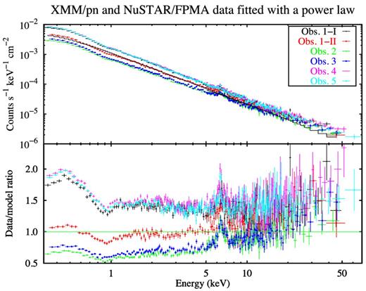
Upper panel: the six XMM–Newton/pn and NuSTAR spectra of NGC 4593. Lower panel: the ratio of the six spectra to a single power law. Only NuSTAR/FPMA data are shown for clarity.
To fully exploit the data set, we always fitted all the XMM–Newton/pn and NuSTAR/FPMA and FPMB data simultaneously, allowing for free cross-calibration constants. The FPMA and FPMB modules are in good agreement with pn, with cross-calibration factors of 1.02 ± 0.01 and 1.05 ± 0.01, respectively, fixing the constant for the pn data to unity. All spectral fits include neutral absorption (phabs model in xspec) from Galactic hydrogen with column density NH = 1.89 × 1022 cm−2 (Kalberla et al. 2005). We assumed the element abundances of Lodders (2003).
The RGS spectra
NGC 4593 is known to host a warm absorber from previous observations with Chandra and XMM–Newton (McKernan et al. 2003; Steenbrugge et al. 2003; Brenneman et al. 2007; Ebrero et al. 2013). The location of this ionized absorber is at least a few pc from the central source (Ebrero et al. 2013), therefore we do not expect it to significantly vary on a few days time-scale. We thus co-added the RGS data from the different epochs, for each detector, to obtain a better signal-to-noise ratio. We fitted the RGS1 and RGS2 co-added spectra in the 0.3–2 keV band. We used a simple model including a power law and the warm absorber. To find a good fit, we needed to include two ionized absorbers, both modelled using the spectral synthesis code cloudy (Ferland et al. 2013). We built a cloudy table model with an allowed range for the ionization parameter log ξ of 0.1–4.9 (in units of erg s−1 cm), while the allowed range for the column density is 1019–1024 cm−2. These ranges are suitable for both absorption components. Starting with a fit including only one absorption component, we find C/dof = 6131/5388. Adding a second component, we find C/dof = 5941/5384 (ΔC/Δdof = −190/−4) and positive residuals around 22 and 29 Å, that may be attributed to the Kα triplets of the He-like ions O vii and N vi. To constrain the parameters of such emission lines, we performed two local fits at the corresponding wavelengths, on intervals ∼100 channels wide. Because of the small bandwidth, the underlying continuum is not sensitive to variations of the photon index. We thus fixed it at 2, leaving free the normalization of the power law. With such fits, we detect four significant (at 90 per cent confidence level) emission lines. We identify the lines as the intercombination (1s2 1S0–1s2p 3P2,1) and forbidden (1s2 1S0–1s2s 3S1) components of the O vii Kα triplet, and the resonance (1s2 1S0–1s2p 1P1) and forbidden components of the N vi Kα triplet (see Table 2). We first modelled these lines using four Gaussian components. After including the lines in the fit over the whole energy range, we find C/dof = 5869/5376 (i.e. ΔC/Δdof = −72/−8). Then, we replaced the Gaussian lines with the emission spectrum from a photoionized plasma, modelled with a cloudy table having the ionization parameter, the column density and the normalization as free parameters. We find a nearly equivalent fit, C/dof = 5866/5379 (ΔC/Δdof = −3/+ 3) and no prominent residuals that can be attributed to strong atomic transitions (see Fig. 3). The best-fitting parameters of the warm absorbers and of the emitter are reported in Table 3.
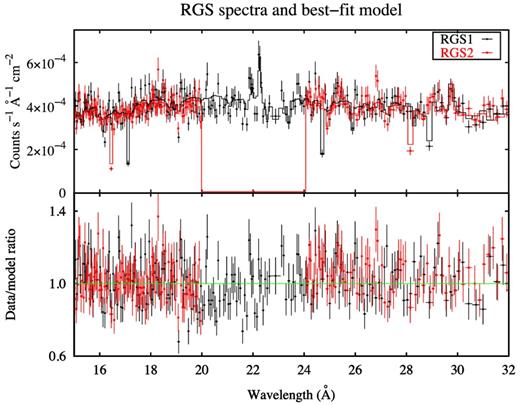
Upper panel: the XMM–Newton/RGS spectra (15–32 Å) with the best-fitting model. Data are rebinned for displaying purposes only. Lower panel: the ratio of the spectra to the model.
The emission lines detected in RGS spectra. λT and ET are the theoretical wavelength and energy of the lines (rest frame), as reported in the atomdb data base (Foster et al. 2012). σ is the intrinsic line width and v is the velocity shift with respect to the systemic velocity of NGC 4593; these two parameters were fixed between lines of the same multiplet. The flux is in units of 10−5 photons cm−2 s−1.
| Line id. | λT (Å) | ET (keV) | σ (eV) | v (km s−1) | Flux |
|---|---|---|---|---|---|
| O vii (f) | 22.091 | 0.561 | |$0.7 ^{+ 0.4 }_{- 0.6 }$| | −450 ± 110 | |$6.2 ^{+ 2.0 }_{- 1.9}$| |
| O vii (i) | 21.795 | 0.569 | – | – | |$2.3 ^{+ 1.8 }_{- 1.6 }$| |
| N vi (r) | 28.738 | 0.431 | <1 | |$-360 ^{+ 270}_{- 180}$| | |$4.0 ^{+ 1.4 }_{- 3.2}$| |
| N vi (f) | 29.528 | 0.420 | – | – | |$4.6 ^{+ 2.7 }_{- 2.1 }$| |
Best-fitting parameters of the warm absorbers (wa1, wa2) and photoionized emission (em) for the RGS spectra. For all these models, ξ is the ionization parameter, σv is the turbulent velocity, NH is the column density and v is the velocity shift with respect to the systemic velocity of NGC 4593; |$N_{\small {em}}$| is the normalization of the photoionized emission table.
| |$\log \xi _{\small {WA}{{1}}}$| (erg s−1 cm) | 2.22 ± 0.01 |
| |$\log \sigma _{v,\small {WA}{{1}}}$| (km s−1) | 1.72 ± 0.07 |
| |$\log N_{\rm{H,}\small {WA}{{1}}}$| (cm−2) | |$21.83 ^{+ 0.07 }_{- 0.02 }$| |
| |$v_{\small {WA}{{1}}}$| (km s−1) | −870 ± 60 |
| |$\log \xi _{\small {WA}{{2}}}$| (erg s−1 cm) | 0.43 ± 0.08 |
| |$\log \sigma _{v,\small {WA}{{2}}}$| (km s−1) | Unconstr. |
| |$\log N_{\rm{H,}\small {WA}{{2}}}$| (cm−2) | 20.90 ± 0.02 |
| |$v_{\small {WA}{{2}}}$| (km s−1) | −300 ± 200 |
| |$\log \xi _{\small {em}}$| (erg s−1 cm) | 0.56 ± 0.03 |
| |$\log \sigma _{v,\small {em}}$| (km s−1) | Unconstr. |
| |$\log N_{\rm{H},\small {em}}$| (cm−2) | >21.4 |
| |$v_{\small {em}}$| (km s−1) | −720 ± 60 |
| |$N_{\small {em}}$| (×10−18) | 6 ± 1 |
The Fe K|$\boldsymbol {\alpha }$| line
We next investigated the properties of the Fe Kα line at 6.4 keV. We focused on XMM–Newton/pn data, given their better energy resolution compared with NuSTAR in that energy band. We fitted the six pn spectra between 3 and 10 keV, to avoid the spectral complexities in the soft X-ray band. The model included a power law plus a Gaussian line at 6.4 keV. Because of a known calibration problem in pn data, the energy of the Gaussian line is blueshifted by ∼50 eV with respect to the theoretical value of 6.4 keV (for a detailed discussion, see Cappi et al. 2016). The shifts vary between different observations and are present using either single plus double or single-only events, despite the use of the latest correction files for charge transfer inefficiency (CTI) and procedure as described in Smith et al. (2014, xmm-ccf-rel-323).1 This is likely an effect of the long-term degradation of the EPIC/pn CTI. To correct for such uncertainty, we fixed the Gaussian line energy at 6.4 keV, implying production by ‘cold’ iron, i.e. less ionized than Fe xii, while leaving the redshift free to vary in pn data. We find an acceptable fit (χ2/dof = 648/571) assuming an intrinsically narrow line, i.e. its intrinsic width σ is fixed at zero. If σ is left free, we find a slightly better fit (χ2/dof = 643/570, i.e. Δχ2/Δdof = −5/−1), with σ = 50 ± 30 eV and a probability of chance improvement (calculated with the F-test) around 0.04.
We then looked for the presence of a broad line component at 6.4 keV. We added a second Gaussian line at 6.4 keV, leaving free the intrinsic width of both lines. The fit improves significantly (χ2/dof = 608/563, i.e. Δχ2/Δdof = −35/−7). The narrow line component has now an intrinsic width consistent with zero, therefore we fixed it at σ = 0. The broad component has |$\sigma =450^{+ 110}_{- 70}$| eV. We report in Figs 4 and 5 the flux and equivalent width of both the narrow and broad components, plotted against the primary flux in the 3–10 keV band. The strong variability of the primary flux is not accompanied by a corresponding variability of the narrow line flux, which is consistent with being constant. As a consequence, the equivalent width is anticorrelated with the primary flux. The Pearson's coefficient is −0.82, with a p value of 4.5 × 10⁻². The broad line flux, instead, shows hints of variability (a fit with a constant gives a reduced χ2 of 1.44), while the equivalent width is consistent with being constant (a fit with a constant gives a reduced χ2 of 0.67; the Pearson's coefficient is −0.55, with a p value of 0.25). However, by including only two Gaussian lines at 6.4 keV, we find positive residuals around 7 keV which could be a potential signature of line emission from ionized iron, such as the Kα line of Fe xxvi at 6.966 keV (rest frame), or of the Kβ line of neutral iron at 7.056 keV. Brenneman et al. (2007) found evidence for a narrow, hydrogen-like Fe Kα emission line in this source by using XMM–Newton/pn data. Markowitz & Reeves (2009) found only an upper limit on the presence of this line by using Suzaku data, but instead found a significant neutral Fe Kβ line. To test for the presence of such components, we included a third, narrow Gaussian line. We kept the line flux tied between different observations. Fixing the line energy at 6.966 keV, we find χ2/dof = 596/573 (Δχ2/Δdof = −20/−1), and no improvement by adding another Gaussian line at 7.056 keV. The fit is only slightly worse if we fix the energy of the third line at 7.056 keV instead of 6.966 keV (Δχ2 = +2). We measure a flux of (6 ± 2) × 10−6 photons cm−2 s−1 for this line, and an equivalent width ranging from 25 ± 10 to 40 ± 20 eV. The ratio of the flux to that of the narrow Fe Kα line is 0.25 ± 0.14, roughly consistent with the predicted ratio of fluorescence yields for Kβ/Kα (∼0.13; see Kaastra & Mewe 1993; Molendi, Bianchi & Matt 2003). Finally, we note that the intrinsic width of the broad component at 6.4 keV is now found to be |$\sigma =300^{+ 130}_{- 70}$| eV, while all the other parameters of the narrow and broad components are not significantly altered by the addition of the third line. We also tried to thaw the energy of the broad component, to test if it could be due to ionized material. However, the fit is not significantly improved, and the line energy is found to be E = 6.44 ± 0.11 keV.
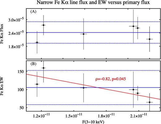
Parameters of the narrow Fe Kα line at 6.4 keV, plotted against the primary flux in the 3–10 keV band. Panel (A): the line flux in units of photons cm−2 s−1. Panel (B): the line equivalent width (EW) in units of eV. Error bars denote the 1σ uncertainty. The blue solid lines represent the mean value for each parameter, while the blue dashed lines represent the standard deviation (i.e. the root mean square of the deviations from the mean). The red line represents a linear fit to the data.
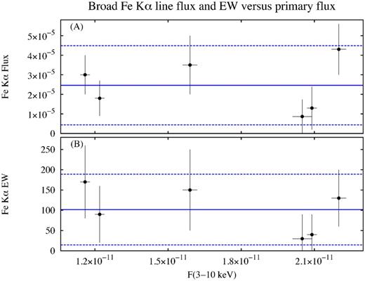
Parameters of the broad Fe Kα line at 6.4 keV, plotted against the primary flux in the 3–10 keV band. Panel (A): the line flux in units of photons cm−2 s−1. Panel (B): the line equivalent width (EW) in units of eV. Error bars denote the 1σ uncertainty. The blue solid lines represent the mean value for each parameter, while the blue dashed lines represent the standard deviation.
Overall, these results are consistent with the cold, narrow Fe Kα line being produced by reflection off relatively distant material, lying at least a few light days away from the nucleus. A statistically significant broad component is detected, showing hints of variability, albeit with no clear trend with respect to the primary flux. The results on the iron lines are summarized in Table 4. Finally, we had a first look at the presence of reflection components associated with the iron lines, using the energy range from 3 up to 79 keV. We fitted the XMM–Newton/pn and NuSTAR data with a simple power law plus three Gaussian emission lines, i.e. the narrow lines at 6.4 and 6.966 keV and the broad component at 6.4 keV, finding χ2/dof = 2084/1923. The residuals indicate the presence of a moderate Compton hump peaking at around 30 keV (see Fig. 6).
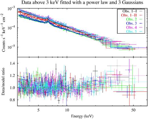
Upper panel: the pn and NuSTAR spectra above 3 keV fitted with a model including a simple power law and three Gaussian lines. Lower panel: the ratio of the spectra to the model, showing an excess around 30 keV. The data were binned for plotting purposes.
| E (keV) | σ (eV) | Average flux | Average EW (eV) |
|---|---|---|---|
| 6.4 (narrow) | 0 | 2.42 | 106 |
| 6.4 (broad) | |$300^{+ 130}_{- 70}$| | 2.36 | 102 |
| 7.056 | 0 | 0.6 | 30 |
| E (keV) | σ (eV) | Average flux | Average EW (eV) |
|---|---|---|---|
| 6.4 (narrow) | 0 | 2.42 | 106 |
| 6.4 (broad) | |$300^{+ 130}_{- 70}$| | 2.36 | 102 |
| 7.056 | 0 | 0.6 | 30 |
| E (keV) | σ (eV) | Average flux | Average EW (eV) |
|---|---|---|---|
| 6.4 (narrow) | 0 | 2.42 | 106 |
| 6.4 (broad) | |$300^{+ 130}_{- 70}$| | 2.36 | 102 |
| 7.056 | 0 | 0.6 | 30 |
| E (keV) | σ (eV) | Average flux | Average EW (eV) |
|---|---|---|---|
| 6.4 (narrow) | 0 | 2.42 | 106 |
| 6.4 (broad) | |$300^{+ 130}_{- 70}$| | 2.36 | 102 |
| 7.056 | 0 | 0.6 | 30 |
The broad-band fit
After getting a clue to the origin of the iron line and to the presence of a reflection component, we fitted the pn and NuSTAR data in the whole X-ray energy range (0.3–79 keV). We modelled the primary continuum with a cut-off power law. The other components are described below. In xspec notation, the model reads: phabs*wa1*wa2*(soft lines + cutoffpl + diskbb + relxill + xillver), where wa1, wa2 and soft lines denote the cloudy tables described in Section 3.1.
The reflection component
In Section 3.2, we found the presence of both a narrow and a broad Fe Kα line components together with a Compton hump. We thus modelled the reflection component with xillver (García & Kallman 2010; García et al. 2013) and relxill (García et al. 2014) in xspec. Both models self-consistently incorporate fluorescence lines and the Compton reflection hump, and in relxill such components are relativistically blurred. We used the xillver-a-ec4 version, which takes into account the angular dependence of the emitted radiation and includes a primary power law with an exponential cut-off up to 1 MeV,2 and the relxill version 0.4c.3 Since the inclination angle of both reflectors was poorly constrained, we fixed it to 50|$^\circ$|, consistently with past studies on this source (Nandra et al. 1997; Guainazzi et al. 1999). We assumed for xillver and relxill the same iron abundance AFe, which was a free parameter of the fit, but tied between the different observations.
In relxill, the normalization was left free to vary between the different observations. The input photon index and cut-off energy were tied to that of the primary power law, as this reflection component was assumed to originate relatively close to the primary source. A priori, also the ionization could change among the observations, responding to the different ionizing flux from the primary source. However, the ionization parameter was always found to be consistent with a common value of log ξ ≃ 3, therefore, we tied this parameter between the different observations. Similarly, the inner radius of the disc was a free parameter of the fit, but tied between the different observations since it was consistent with being constant. Since the emissivity index was poorly constrained, we fixed it at 3 (the classical case; see e.g. Wilkins & Fabian 2012). We found no improvement by assuming a broken power law for the emissivity profile. Moreover, since the black hole spin parameter a was poorly constrained, we assumed a = 0.998.
The xillver component was consistent with being constant, being associated with the narrow, constant component of the Fe Kα line. The normalization was a free parameter of the fit, but tied between the different observations. Since the input photon index and cut-off energy of xillver were poorly constrained, we fixed them to the average values of the photon indexes and of the cut-off energies of the primary power law found in each observation. We fixed the ionization parameter at the minimum value in xillver, log ξ = 0, with no improvement by leaving it free.
We also tested the possibility that the iron line and the reflection hump are not directly correlated. We thus included an additional narrow Gaussian line at 6.4 keV, not related to the reflection components. Such a line could originate from Compton-thin gas, which does not produce a significant Compton hump (e.g. Bianchi et al. 2008). However, the fit is only marginally improved, and the parameters of the reflection components are not significantly altered. Therefore, for the sake of simplicity, we included only xillver and relxill in our model.
The warm absorber and soft lines
Following Section 3.1, we included two ionized absorbers and the soft X-ray emission lines found with RGS, modelled with cloudy. To account for cross-calibration uncertainties between pn and RGS, especially below 0.5 keV, the parameters of the absorbers were left free, but kept constant between the different observations. We found no significant improvement by leaving the warm absorber free to vary between the different observations. The cloudy table for the emission lines was fixed to the RGS best-fitting values, as it was poorly constrained by pn data. This reflected spectrum also adds a weak contribution in the hard X-ray band, because it produces self-consistently an iron line and a reflection hump (see Fig. 7).
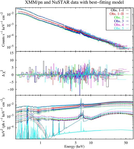
Broad-band X-ray data and best-fitting model (see Table 5). Upper panel: XMM–Newton/pn and NuSTAR data and folded model. Middle panel: contribution to χ2. Lower panel: best-fitting model E2f(E), with the plot of the reflection components xillver (dotted line) and relxill (dashed lines), the cloudy model for the soft emission lines with associated reflected continuum (solid line) and the diskbb component for the soft excess (dotted lines). The data were rebinned for plotting purposes.
We also tested a partial covering scenario for the warm absorbers. However, we find that if the covering fraction of both components is allowed to vary, it is consistent with 1.
The soft excess
Ionized reflection alone does not explain all the observed soft excess in this source, because including only the reflection components leaves strong, positive residuals below 1 keV. We modelled the soft excess phenomenologically with a multicolour disc blackbody component, through the diskbb model in xspec (Mitsuda et al. 1984; Makishima et al. 1986). The normalization was left free to vary between different observations, while the inner disc temperature was found to be consistent with a common value of around 110 eV, thus it was tied between the different observations.
In Fig. 7 we show the data, residuals and best-fitting model, while all the best-fitting parameters are reported in Table 5. According to our results, the unblurred reflection component (xillver) is consistent with being constant and due to neutral matter. The reflection strength, |$\mathcal {R}_{\rm s,\small {xillver}}$|, calculated as the ratio between the 20–40 keV flux of the xillver component and the 20–40 keV primary flux, ranges between ∼0.35 and ∼0.6. This ratio is slightly different from the traditional reflection fraction |$\mathcal {R}_{\rm f}=\Omega /2\pi$|, where Ω is the solid angle subtended by the reflector (Magdziarz & Zdziarski 1995). We discuss this further in Section 4. The blurred component (relxill) is due to an ionized disc with ξ ∼ 1000 erg s−1 cm, and with an inner radius Rin ≃ 40 RG. The reflection strength |$\mathcal {R}_{\rm s,\small {relxill}}$|, i.e. the ratio between the 20–40 keV flux of relxill and that of the 20–40 keV primary flux, ranges between ∼0.15 and ∼0.25. Analogous results are found calculating the ratio between fluxes in a broader energy range, such as 0.1–100 keV (e.g. Wilkins et al. 2015). With this choice, we find similar values for |$\mathcal {R}_{\rm s,\small {relxill}}$|, while for |$\mathcal {R}_{\rm s,\small {xillver}}$| we find 0.15–0.35. However, using the 20–40 keV range is likely more appropriate, as the reflection spectrum in that band is dominated by Compton scattering, only weakly depending on the iron abundance or the ionization state (Dauser et al. 2016). We also estimated the equivalent width of the broad iron line associated with relxill, finding values consistent with those measured in Section 3.2, namely 100–150 eV.
Best-fitting parameters of the broad-band (0.3–80 keV) phenomenological model described in Section 3.3: wa1*wa2*(soft lines + cutoffpl + diskbb + relxill + xillver). In the second column we report the fit parameters that were kept constant, i.e. they were constrained by all observations. In the third to eighth columns, we report the fit parameters that were free to vary for each observation. In the last column, we report the best-fitting parameters for the summed spectra. Parameters in italics were frozen due to poor constraints.
| All obs. | Obs. 1-I | Obs. 1-II | Obs. 2 | Obs. 3 | Obs. 4 | Obs. 5 | Summed | |
|---|---|---|---|---|---|---|---|---|
| |$\log \xi _{\small {wa1}}$| | 2.71 ± 0.05 | |$2.70 ^{+ 0.09 }_{- 0.05 }$| | ||||||
| |$\log \sigma _{v,\small {wa1}}$| | >2.2 | |$\mathit {2.5}$| | ||||||
| |$\log N_{\rm{H,}\small {wa1}}$| | 21.4 ± 0.1 | 21.4 ± 0.1 | ||||||
| |$\log \xi _{\small {wa2}}$| | |$\mathit {0.1}$| | |$\mathit {0.1}$| | ||||||
| |$\log \sigma _{v,\small {wa2}}$| | |$2.01^{+ 0.01}_{- 0.05}$| | |$2.2 ^{+ 0.2 }_{- 0.4 }$| | ||||||
| |$\log N_{\rm{H,}\small {wa2}}$| | |$21.09^{+ 0.01}_{- 0.07}$| | |$21.13 ^{+ 0.02 }_{- 0.03 }$| | ||||||
| Γ | 1.85 ± 0.01 | 1.69 ± 0.02 | |$1.59^{+ 0.03}_{- 0.02}$| | |$1.65^{+ 0.01}_{- 0.02}$| | 1.82 ± 0.01 | 1.83 ± 0.01 | 1.84 ± 0.01 | |
| Ec (keV) | >700 | |$170^{+ 160}_{- 60}$| | |$90^{+ 40}_{- 20}$| | |$170^{+ 70}_{- 40}$| | |$470^{+ 430}_{- 150}$| | >450 | >640 | |
| |$N_{\small {pow}}\ (\times 10^{-3})$| | |$7.1^{+ 0.2}_{- 0.1}$| | 4.4 ± 0.2 | |$2.5^{+ 0.2}_{- 0.1}$| | 2.9 ± 0.1 | 7.1 ± 0.2 | |$7.0^{+ 0.2}_{- 0.1}$| | 5.4 ± 0.1 | |
| |$kT_{\small {diskbb}}$| (eV) | 110 ± 3 | |$105 ^{+ 4}_{- 3}$| | ||||||
| |$N_{\small {diskbb}}\ (\times 10^3)$| | |$6.8^{+ 0.2}_{- 0.3}$| | |$4.1^{+ 0.3}_{- 0.2}$| | |$2.7^{+ 0.1}_{- 0.2}$| | |$2.9^{+ 0.2}_{- 0.1}$| | |$7.6^{+ 0.3}_{- 0.2}$| | 7.7 ± 0.2 | 7.5 ± 1.61. | |
| |$\log \xi _{\small {relxill}}$| | |$3.00^{+ 0.01}_{- 0.13}$| | |$2.93^{+ 0.08 }_{- 0.11 }$| | ||||||
| Rin (RG) | 40 ± 15 | |$40 ^{+ 15 }_{- 30 }$| | ||||||
| |$N_{\small {relxill}}\ (\times 10^{-5})$| | 3.1 ± 0.7 | 2.5 ± 0.5 | 2.4 ± 0.3 | 2.6 ± 0.3 | |$4.6^{+ 0.6}_{- 0.5}$| | |$4.2^{+ 0.4}_{- 0.5}$| | |$3.3 ^{+ 0.7 }_{- 0.5 }$| | |
| |$N_{\small {xillver}}\ (\times 10^{-5})$| | 2.5 ± 0.3 | |$3.1 ^{+ 0.3 }_{- 0.4 }$| | ||||||
| AFe | |$2.6^{+ 0.2}_{- 0.4}$| | 2.0 ± 0.3 | ||||||
| χ2/dof | 2506/2299 | 2401/2264 | ||||||
| Individual χ2/dof | 383/362 | 389/340 | 380/376 | 404/387 | 491/426 | 459/421 |
Concerning the primary continuum, we find significant variations of the photon index (up to ΔΓ ≃ 0.2) and of the high-energy cut-off. The contour plots of the cut-off energy versus photon index are shown in Fig. 8. To check the significance of the cut-off energy variability, we repeated the fit keeping the cut-off energy Ec tied between the different observations. We find |$E_{\rm{c}}=420^{+ 400}_{- 130}$| keV, however the fit is significantly worse (Δχ2/Δdof = +48/+5 with a p value of 3 × 10⁻⁸ from an F-test). We also performed a fit to the co-added pn and NuSTAR spectra (see Table 5), finding a photon index of 1.84 ± 0.01 and a cut-off energy >640 keV. More importantly, the parameters are consistent with those that were kept constant in the simultaneous fit of the single observations.
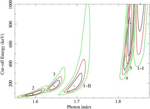
Contour plots of the primary continuum cut-off energy versus photon index for each observation (see also Table 5). Green, red and black lines correspond to 99, 90 and 68 per cent confidence levels, respectively.
A multicolour disc blackbody with an inner temperature of ∼110 eV is found to describe well the soft excess seen on top of the primary power law and of the ionized reflection component. We note that, if the primary power law is due to Comptonization, it should have a low-energy roll-over dependent on the temperature of the seed photons, which could enhance the soft excess. However, if the seed photons are in the optical/UV band, the effect is negligible when fitting the data above 0.3 keV (see also the discussion in Section 4). We also found a significant correlation between the soft excess flux and the primary emission. We show in Fig. 9 the 3–10 keV flux of the primary power law, the 10–50 keV flux and the photon index, plotted against the diskbb flux in the 0.3–2 keV band. The correlation between the diskbb flux and the soft primary flux has a Pearson's coefficient of 0.98 and a p value of 8 × 10⁻⁴. For the hard band, the Pearson's coefficient is 0.95, with a p value of 3.3 × 10⁻³. For the photon index, the Pearson's coefficient is 0.97, with a p value of 1.8 × 10⁻³. A detailed modelling of the soft excess is beyond the scope of this paper, and it is deferred to a following paper.
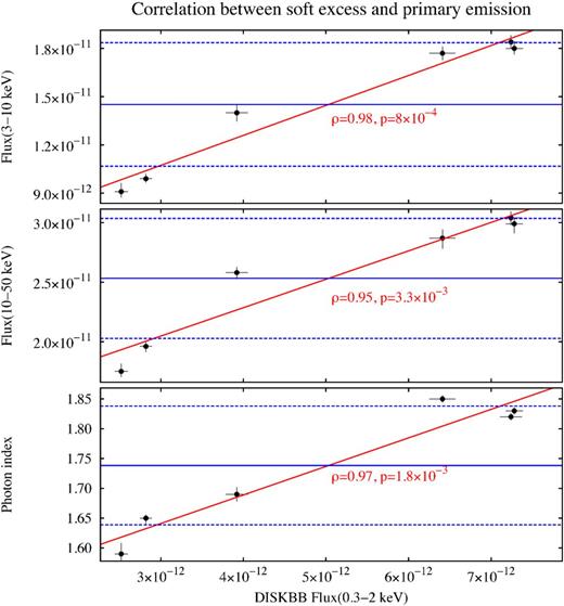
Three parameters of the primary power law plotted against the flux of the soft excess (calculated as the 0.3–2 keV flux of the diskbb component, see Section 3.3). Upper panel: primary flux in the 3–10 keV range. Middle panel: primary flux in the 10–50 keV range. Lower panel: primary photon index. All fluxes are in units of erg s−1 cm−2. The blue solid lines represent the mean value for each parameter, while the blue dashed lines represent the standard deviation. The red lines represent linear fits to the data.
DISCUSSION AND CONCLUSIONS
We reported results based on a joint XMM–Newton and NuSTAR monitoring of NGC 4593, aimed at studying the broad-band variability of this AGN in detail.
The source shows a remarkable variability, both in flux and in spectral shape, on time-scales of a few days and down to a few ks. While flux variability is significant at all energies, the spectral variability is mostly observed below 10 keV. Moreover, the spectrum is softer when the source is brighter, as generally found in luminous Seyfert galaxies (e.g. Markowitz, Edelson & Vaughan 2003; Sobolewska & Papadakis 2009; Soldi et al. 2014). If the X-ray emission is produced by Comptonization, the relation between observed flux and photon index can be understood as an effect of that process. The spectral shape primarily depends on the optical depth and temperature of the Comptonizing corona, albeit in a non-trivial way (e.g. Sunyaev & Titarchuk 1980). The photon index can be also related to the Compton amplification ratio, i.e. the ratio between the total corona luminosity and the soft luminosity that enters and cools the corona. A higher amplification ratio corresponds to a harder spectrum (e.g. Haardt & Maraschi 1993). In the limiting case of a ‘passive’ disc, which is not intrinsically radiative but rather reprocesses the coronal emission, the amplification ratio is fixed by geometry alone (e.g. Haardt & Maraschi 1991; Stern et al. 1995). Then, in steady states (i.e. the system is in radiative equilibrium), the coronal optical depth and temperature adjust to keep the amplification ratio constant. But the amplification ratio can change following geometry variations of the accretion flow. For example, the inner radius of the disc may be different from the innermost stable circular orbit (as suggested by the fit with the relativistic reflection) and change in time,4 causing a decrease of the soft luminosity supplied by the disc. This, in turn, may increase the amplification ratio, leading to a harder spectrum. This kind of behaviour is especially apparent during Obs. 1, where a significant flux drop (a factor of ∼2 in the 0.5–2 keV count rate) is accompanied by a significant hardening of the spectrum (ΔΓ ≃ 0.15).
However, we also find a significantly variable high-energy cut-off (see Fig. 8). In particular, the lowest cut-off is seen during Obs. 2, where |$E_{\rm{c}}=90^{+ 40}_{- 20}$| keV. This corresponds to the hardest spectrum, with Γ ≃ 1.6. For the softest spectra, like Obs. 1-I and Obs. 5, we only find a lower limit on Ec of several hundreds of keV. Since the cut-off energy is generally related to the coronal temperature (Ec ≃ 2–3 kT; e.g. Petrucci et al. 2001), our results might suggest that this temperature undergoes huge variations (from a few tens up to a few hundreds of keV) during a few days. However, it should be noted that the turnover of a Comptonized spectrum is much sharper than a simple exponential cut-off (e.g. Zdziarski et al. 2003). Then, fitting the data with a cut-off power law provides only a phenomenological description that does not allow for an unambiguous physical interpretation (e.g. Petrucci et al. 2001).
We confirm the presence of a warm absorber affecting the soft X-ray spectrum. Ebrero et al. (2013), using a 160 ks Chandra data set, found evidence for a multiphase ionized outflow with four distinct degrees of ionization, namely log ξ = 1.0, 1.7, 2.4 and 3.0. The low-ionization components were found to have lower velocities (300–400 km s−1) than the high-ionization components (up to ∼1000 km s−1). According to our results, a two-phase ionized outflow provides an adequate characterization of this gas, both for RGS and pn spectra. These two components have different degrees of ionization, namely log ξ ≃ 2.2–2.5 and 0.1–0.4, and different column densities, NH ≃ (2–7) × 1021 and (0.8–1.2) × 1021 cm−2, with uncertainties due to the different estimates based on pn and RGS data. The two components are also kinematically distinct, with the high-ionization component outflowing faster (v ≃ −900 km s−1) than the low-ionization one (v ≃ −300 km s−1). We can derive a rough upper limit on the distance of such components in the following way (see also Ebrero et al. 2013). By definition, ξ = Lion/nR2, where Lion is the ionizing luminosity in the 1–1000 Ryd range, n is the hydrogen gas density and R the distance. If we assume that the gas is concentrated within a layer with thickness Δr ≤ R, we can write R ≤ Lion/NHξ, where NH = nΔr. The average ionizing luminosity that we obtain from our best-fitting model is ∼1 × 1043 erg s−1. Then, from the measurements of NH and ξ we get an upper limit on R. For the high-ionization component we estimate R ≲ 3 pc, while for the low-ionization component R ≲ 1.5 kpc. The outflows are thus consistent with originating at different distances from the nucleus, as found by Ebrero et al. (2013), with the high-ionization and high-velocity component possibly being launched closer to the central source.
We find evidence for a cold, narrow Fe Kα line which is consistent with being constant during the monitoring. A broad component is also detected, and is consistent with originating at a few tens of gravitational radii from the black hole. The Fe Kα line is accompanied by a moderate Compton hump (the total reflection strength is approximately 0.5–0.8). All these features are well modelled by including two different reflection components, both requiring an iron overabundance of 2–3. One component (xillver) is responsible for the narrow core of the Fe Kα line, and is consistent with arising from a slab of neutral, Compton-thick material. This component is also consistent with being constant, despite the observed strong variability of the primary continuum. The variability of the primary emission can be diluted in a distant reflector, if the light-crossing time across the reflecting region is more than the variability time-scale of the primary continuum. In this case, the reflector responds to a time-averaged illumination from the primary source. Therefore, the reflecting material should lie at least a few light days away from the primary source, and it can be interpreted as the outer part of the accretion disc. The reflection strength |$\mathcal {R}_{\rm s,\small {xillver}}$|, namely the ratio between the reflected and the primary flux in the 20–40 keV band, is in the range 0.35–0.6. According to Dauser et al. (2016), the reflection strength is likely an underestimate of the reflection fraction |$\mathcal {R}_{\rm f}$|, defined as the ratio between the primary intensity illuminating the disc and the intensity reaching the observer. The difference is that |$\mathcal {R}_{\rm s}$| depends on the inclination of the reflector, while |$\mathcal {R}_{\rm f}$| does not. For an isotropic source, |$\mathcal {R}_{\rm f}=\Omega / 2\pi$|, where Ω is the solid angle covered by the reflector as seen from the primary source. Dauser et al. (2016) report |$\mathcal {R}_{\rm s} \simeq 0.7$| when |$\mathcal {R}_{\rm f}$| is set to 1 in xillver, for an inclination angle of 50|$^\circ$|. Therefore, in our case, we estimate |$\mathcal {R}_{\rm f,\small {xillver}}$| to be in the range 0.5–0.85. This would correspond to a solid angle between π and 1.7π. However, there are a few caveats. First, if the reflecting material is more distant (e.g. a torus at pc scales), the reflection fraction might not be closely related to the viewing angle (e.g. Malzac & Petrucci 2002). Furthermore, the X-ray emitting corona could be outflowing or inflowing rather than being static (Beloborodov 1999; Malzac, Beloborodov & Poutanen 2001). In this case, the reflection fraction would depend also on the velocity of the corona, because the relativistic beaming would result in an anisotropic illumination (Malzac et al. 2001).
The second reflection component (relxill) is responsible for the broad Fe Kα line, and is consistent with originating from the inner part of the accretion disc, down to ∼40RG. Given the black hole mass of ∼1 × 10⁷ solar masses, a distance of 40RG corresponds to a light-travel time of ∼2 ks. Indeed, this reflection component appears to respond to the variability of the primary continuum (see Table 5 and Fig. 5 from the phenomenological fit of the broad Fe Kα line with a Gaussian component). A more detailed discussion is deferred to a forthcoming paper, where a timing analysis will be performed (B. De Marco et al., in preparation). The reflection strength |$\mathcal {R}_{\rm s,\small {relxill}}$| is ∼0.2, and the effects of light bending in relxill may complicate the geometrical interpretation (Dauser et al. 2016). However, given the relatively large inner disc radius, we do not expect a strong modification of the reflection fraction (e.g. Dauser et al. 2014). Using the same relations as for xillver, we find a covering angle Ω ≃ π. Finally, our results suggest that a slightly larger |$\mathcal {R}_{\rm s,\small {relxill}}$| corresponds to the low-flux states, i.e. to a flatter Γ, whereas a correlation between the photon index and the reflection fraction is usually found in AGN (e.g. Zdziarski, Lubiński & Smith 1999; Malzac & Petrucci 2002). According to Zdziarski et al. (1999), a correlation can be explained if the reflecting medium is also the source of seed soft photons that get Comptonized in the hot corona. In our case, the lack of such a correlation and the presence of a strong soft excess suggest that the source of soft photons and the reflecting medium are not one and the same.
The soft X-ray excess is phenomenologically well described by a variable multicolour disc blackbody. Physically, the soft excess could be produced by a warm corona upscattering the optical/UV photons from the accretion disc (see e.g. Magdziarz et al. 1998; Petrucci et al. 2013). This warm corona could be the upper layer of the disc (e.g. Różańska et al. 2015). The observed correlation between the flux of the soft excess and that of the primary power law (Fig. 9) could indicate that these two components arise from the Comptonization of the same seed photons. Then, the observed correlation between the soft excess and the primary photon index can be seen as a simple consequence of the flux correlation and of the softer-when-brighter behaviour of the primary continuum. However, the actual scenario could be more complex. Assuming that the soft excess is produced by a warm corona, part of this emission (depending on geometry) could be in turn upscattered in the hot corona and contribute to its Compton cooling. In this case, a larger flux from the warm corona would imply a more efficient cooling of the hot corona, thus a softer X-ray emission. These results motivate a further, detailed investigation using realistic Comptonization models, which will be the subject of a forthcoming paper.
We thank the anonymous referee for helpful comments and suggestions that improved the paper.
This work is based on observations obtained with: the NuSTAR mission, a project led by the California Institute of Technology, managed by the Jet Propulsion Laboratory and funded by NASA; XMM–Newton, an ESA science mission with instruments and contributions directly funded by ESA Member States and the USA (NASA). This research has made use of data, software and/or web tools obtained from NASA's High Energy Astrophysics Science Archive Research Center (HEASARC), a service of Goddard Space Flight Center and the Smithsonian Astrophysical Observatory. FU, P-OP, GM, SB, MC, ADR and JM acknowledge support from the French–Italian International Project of Scientific Collaboration: PICS-INAF project number 181542. FU and P-OP acknowledge support from CNES. FU acknowledges support from Université Franco-Italienne (Vinci PhD fellowship). FU and GM acknowledge financial support from the Italian Space Agency under grant ASI/INAF I/037/12/0-011/13. P-OP acknowledges financial support from the Programme National Hautes Energies. SB, MC and ADR acknowledge financial support from the Italian Space Agency under grant ASI-INAF I/037/12/P1. GP acknowledges support by the Bundesministerium für Wirtschaft und Technologie/Deutsches Zentrum für Luft und Raumfahrt (BMWI/DLR, FKZ 50 OR 1408) and the Max Planck Society.
We do not detect significant variations of the inner radius of the relxill reflection component. However, given the uncertainty, we cannot exclude variations by up to a factor of 2 (from ∼25 to ∼50RG).
REFERENCES
