


Abstract
We present 3.7 arcsec (∼0.05 pc) resolution 3.2 mm dust continuum observations from the Institut de Radioastronomie Millimétrique Plateau de Bure Interferometer, with the aim of studying the structure and fragmentation of the filamentary infrared dark cloud (IRDC) G035.39–00.33. The continuum emission is segmented into a series of 13 quasi-regularly spaced (λobs ∼ 0.18 pc) cores, following the major axis of the IRDC. We compare the spatial distribution of the cores with that predicted by theoretical work describing the fragmentation of hydrodynamic fluid cylinders, finding a significant (a factor of ≳ 8) discrepancy between the two. Our observations are consistent with the picture emerging from kinematic studies of molecular clouds suggesting that the cores are harboured within a complex network of independent sub-filaments. This result emphasizes the importance of considering the underlying physical structure, and potentially, dynamically important magnetic fields, in any fragmentation analysis. The identified cores exhibit a range in (peak) beam-averaged column density (3.6 × 1023 cm−2 < NH, c < 8.0 × 1023 cm−2), mass (8.1 M⊙ < Mc < 26.1 M⊙), and number density (6.1 × 105 cm−3 < nH, c, eq < 14.7 × 105 cm−3). Two of these cores, dark in the mid-infrared, centrally concentrated, monolithic (with no traceable substructure at our PdBI resolution), and with estimated masses of the order ∼20–25 M⊙, are good candidates for the progenitors of intermediate-to-high-mass stars. Virial parameters span a range 0.2 < αvir < 1.3. Without additional support, possibly from dynamically important magnetic fields with strengths of the order of 230 μG < B < 670 μG, the cores are susceptible to gravitational collapse. These results may imply a multilayered fragmentation process, which incorporates the formation of sub-filaments, embedded cores, and the possibility of further fragmentation.
INTRODUCTION
Although a basic mechanism for the specific case of isolated low-mass star formation has been investigated over several decades (e.g. Shu, Adams & Lizano 1987), a more generalized model, one that incorporates a consistent description for the formation of high-mass (>8 M⊙) stars, is still lacking. An important step in developing a holistic understanding of the star formation process is identifying and categorising the initial phases of high-mass star formation. Ultimately this requires detailed knowledge of their host molecular clouds.
Discovered as silhouettes against the bright Galactic mid-infrared background, infrared dark clouds (hereafter, IRDCs) were quickly identified as having the potential to aid our understanding of the star formation process (Pérault et al. 1996; Egan et al. 1998). Initial studies set about categorizing their physical properties, finding broad ranges in size (∼1–10 pc, with rare examples exceeding 50 pc e.g. ‘Nessie’; Jackson et al. 2010), mass (102–105 M⊙), and column density (∼1022–1025 cm−2) (e.g. Carey et al. 1998; Egan et al. 1998; Rathborne, Jackson & Simon 2006; Simon et al. 2006). Subsequent investigations categorizing their temperatures (≲ 25 K; Pillai et al. 2006; Peretto et al. 2010; Ragan, Bergin & Wilner 2011; Fontani et al. 2012; Chira et al. 2013), chemistry (e.g. Sakai et al. 2008; Gibson et al. 2009; Jiménez-Serra et al. 2010; Vasyunina et al. 2011; Sanhueza et al. 2012, 2013; Pon et al. 2015; Lackington et al. 2016), and kinematics (e.g. Devine et al. 2011; Henshaw et al. 2013, 2014; Peretto et al. 2013, 2014; Tackenberg et al. 2014; Dirienzo et al. 2015; Schneider et al. 2015; Pon et al. 2016) have ensued. Although the broad range in characteristics dictates that not all IRDCs will form high-mass stars (Kauffmann & Pillai 2010), identifying massive and relatively quiescent molecular clouds (those that are yet to be globally influenced by feedback effects from massive young stellar objects) is a crucially important step in understanding the initial conditions for high-mass star formation.
The focus of this paper is G035.39–00.33, a massive (∼2 × 10⁴ M⊙; see table 1 of Kainulainen & Tan 2013) and filamentary IRDC, with a kinematic distance of 2.9 kpc (Simon et al. 2006). Originally part of a sample selected from the Rathborne et al. (2006) study by Butler & Tan (2009), G035.39–00.33 was selected for further investigation due to its high-contrast against the Galactic mid-infrared background, and because it exhibits extended regions with no obvious tracers of star formation activity (4.5, 8, and 24 μm emission; Carey et al. 2009; Chambers et al. 2009). Since 2010, G035.39–00.33 has been the focal point of a dedicated research effort whose aim is to provide a detailed case study of the physical structure, chemistry, and dynamics of a single IRDC.
The first results of this case study were presented by Jiménez-Serra et al. (2010, Paper I), who identified faint, but widespread, SiO emission throughout G035.39–00.33. Although a currently undetected population of low-mass protostars may account for this emission, Jiménez-Serra et al. (2010) discussed the possibility that such a signature may represent a ‘fossil record’ of either the cloud formation process or a cloud merger.
The potential to use G035.39–00.33 as a laboratory for studying the early phases of the star formation process is supported by both Hernandez et al. (2011, Paper II) and Barnes et al. (2016, Paper VII), who report widespread depletion of CO and widespread emission from deuterated species (in this case, N2D+), respectively. These two observations emphasize the presence of cold (<20 K) and dense gas, yet to be globally affected by stellar feedback, where CO molecules have frozen on to the surface of dust grains leading to an enhancement in the abundance of deuterated nitrogen-bearing molecules. Comparing the observed abundance of deuterated species with that predicted by chemical models (Kong et al. 2015), Barnes et al. (2016) estimate the age of the cloud to be ∼3 Myr old. This may imply, therefore, that although star formation within the cloud remains within an early evolutionary phase, the cloud itself is dynamically old. Having existed for 5–10 local free-fall times, G035.39–00.33 may have had sufficient time to settle into a state of near virial equilibrium, as concluded by Hernandez et al. (2012, Paper III).
The results of Jiménez-Serra et al. (2010) implied that G035.39–00.33 comprises multiple sub-clouds. This was investigated by both Henshaw et al. (2013, Paper IV) and Jiménez-Serra et al. (2014, Paper V), who performed systematic studies of the kinematics and structure of G035.39–00.33. On the largest scales, at least three line-of-sight kinematic features are present, with each exhibiting a unique velocity and density structure (Jiménez-Serra et al. 2014). This was confirmed by Henshaw et al. (2014, Paper VI), who performed the first high angular resolution (∼5 arcsec) study of the dense gas kinematics throughout the cloud, using observations of the J = 1 → 0 transition of N2H+ taken with the Plateau de Bure Interferometer (hereafter, PdBI). It was revealed that the IRDC comprises a complex network of morphologically distinct molecular filaments. Moreover, Henshaw et al. (2014) found evidence to suggest that the kinematics of the gas are locally influenced by the presence of dense, and in some cases, starless, continuum sources.
In this paper (VIII), we revisit the PdBI 3.2 mm continuum emission data, which was first presented by Henshaw et al. (2014) for qualitative comparison with the N2H+ (1−0) molecular line kinematics. Our primary aim is to investigate the structure, fragmentation process, and star formation potential of G035.39–00.33 via quantitative analysis of the dust continuum emission. Details of the observations can be found in Section 2. In Section 3, we discuss the method used to systematically identify structure within the continuum data and discuss this in the context of the complex kinematics of G035.39–00.33. Section 4 contains our quantitative analysis of the continuum data. We begin with a discussion on the spatial distribution of the identified continuum cores and how this compares to predictions from theoretical work describing the fragmentation of fluid cylinders, before turning our attention to the cores themselves. In Section 5, we discuss the implications of our findings in the context of star formation throughout G035.39–00.33. Finally, in Section 6 we summarize our findings and suggest possible avenues for future research.
OBSERVATIONS
The 3.2 mm continuum observations were carried out using the Institut de Radioastronomie Millimétrique (IRAM) PdBI, France. A 6-field mosaic was used to cover the inner area of IRDC G035.39–00.33 (the dotted circles in Fig. 1 depict the primary beam of the PdBI at 3.2 mm ∼54 arcsec). The final map size is ∼40 arcsec × 150 arcsec (corresponding to ∼0.6 pc × 2.1 pc).

The combined mid- and near-infrared extinction-derived mass surface density map of Kainulainen & Tan (2013, grey-scale) overlaid with 3.2 mm continuum contours. Contour levels start at 3σrms and increase in steps of 2σrms (where σrms ≈ 0.07 mJy beam−1). Large dotted circles indicate the 6-field mosaic obtained with the PdBI. Filled magenta circles indicate the locations of high-mass cores reported by Butler & Tan (2012). Filled cyan and yellow squares refer to the high-mass (>20M⊙) and low-mass (<20M⊙) dense cores identified by Nguyen Luong et al. (2011) from Herschel observations. Open red circles and red triangles refer to the 8, and 24 μm emission, respectively (Carey et al. 2009; Jiménez-Serra et al. 2010). The symbol sizes are scaled by the source flux. Filled green squares highlight the location of extended 4.5 μm emission (Chambers et al. 2009).
Observations were carried out over six days in 2011 May, June, and October, in the C and D configurations (using six and five antennas, respectively) offering baselines between 19 m and 176 m. Emission on scales larger than ∼1.2(λ/D) ∼ 42 arcsec (∼0.6 pc), where D = 19 m, is filtered out by the interferometer. The 3.2 mm continuum data were cleaned using the hogbom algorithm with natural weighting. This results in a synthesized beam of {θmaj, θmin} = {4.3 arcsec, 3.1 arcsec} = {0.06 pc, 0.04 pc}, with a position angle of 18|$_{.}^{\circ}$|3. Line-free channels give a total bandwidth of ∼ 3 GHz. The map noise level, σrms, estimated from emission free regions, is ∼0.07 mJy beam−1. The reference position used to determine the relative offset positions used throughout this paper is |$\alpha \,({\rm J}2000)=18^{\rm h}57^{\rm m}08{^{\rm s}_{.}}0$|, δ (J2000) = 02°10′30|${^{\prime\prime}_{.}}$|0. We refer the reader to Henshaw et al. (2014) for more details on the observations.
In addition to the 3.2 mm continuum data, complementary PdBI N2H+ (1−0) observations, first presented in Henshaw et al. (2014), are also utilized throughout this work. These data have been combined with existing IRAM 30 m observations to incorporate missing short spacing information into the interferometric map. Following post-processing, the spatial and spectral resolution of the N2H+ (1−0) data are ∼5 arcsec and 0.14 km s−1, respectively.
OBSERVATIONAL RESULTS
Structure identification using continuum data
Fig. 1 shows the spatial extent of the PdBI 6-field mosaic (dotted circles) overlaid on the combined mid- and near-infrared extinction-derived mass surface density map of G035.39–00.33 (Kainulainen & Tan 2013). The black contours highlight the 3.2 mm continuum emission. The locations of extended 4.5 (extended green objects; Cyganowski et al. 2008), 8, and 24 μm emission, indicating locations of embedded star formation, appear as green squares, red circles, and red triangles, respectively (Carey et al. 2009; Chambers et al. 2009; Jiménez-Serra et al. 2010). Qualitatively, the continuum emission appears closely related to regions of high-mass surface density (0.15 g cm−2 < Σ < 0.32 g cm−2). However, there are notable exceptions to this. For instance, there is a lack of continuum emission towards {Δα, Δδ} = { − 20.0 arcsec, 70.0 arcsec}. Such discrepancies may be due to a lack of sensitivity (our 3σrms column density sensitivity is NH ≳ 1023cm−2; see Section 4.2) or the result of missing short spacings in our interferometric map.
The continuum emission is highly structured. There are a number of prominent emission peaks arranged along the major axis of the IRDC. To investigate this further, we use dendrograms (Rosolowsky et al. 2008). Specifically, our analysis makes use of astrodendro, a python package used to compute dendrograms of astronomical data.1 As well as providing a systematic approach to structure identification, dendrograms are also less sensitive to variation in the input parameters in comparison to alternative methods (Pineda, Rosolowsky & Goodman 2009). Additionally, dendrograms can be used to identify hierarchical structure, which is desirable in complex regions. The following parameters are used in computing the dendrogram: |${\rm min\_value}= 3\sigma _{\rm rms}$| (the minimum intensity considered in the analysis); |${\rm min\_delta}= 2\sigma _{\rm rms}$| (the minimum spacing between isocontours; using |${\rm min\_delta}= 1\sigma _{\rm rms}$| has no effect on the identified structure); |${\rm min\_npix}=26$| (the minimum number of pixels contained within a structure). The angular resolution of our observations is used to determine |${\rm min\_npix}=\frac{2\pi }{8{\rm ln}(2)}\frac{\theta _{\rm maj}\theta _{\rm min}}{A_{\rm pix}}$|, where Apix is the area of a single (0.76 arcsec × 0.76 arcsec) pixel.
Fig. 2 shows the result of the dendrogram analysis. Here we highlight the location of the dendrogram ‘leaves’, the highest level of the dendrogram hierarchy, representing the smallest structures identified. A total of 13 leaves are identified. Each is denoted by an ID number designated in order of increasing offset declination. Equivalent radii of the leaves range between 0.04 pc < Req < 0.07 pc (with a median value of Req = 0.05 pc; note that |$\sqrt{\theta _{\rm maj}\theta _{\rm min}}\sim 3.7$| arcsec which is ∼0.05 pc), whereby Req ≡ (NpixApix/π)1/2, and Npix is the number of pixels associated with a given leaf. The equivalent radius refers to that of a circle which covers an area equivalent to NpixApix. These radii are, on average, 30 per cent larger than the geometric mean radii computed from the intensity-weighted second moment output from astrodendro (see Table 1 and discussion by Rosolowsky & Leroy 2006). Selecting the equivalent radius therefore represents a conservative approach to estimating the physical properties of the leaves (e.g. number densities; Section 4.2). The median aspect ratio of the dendrogram leaves is 2.2. However, leaves #4 and #5 appear to be more filamentary, with aspect ratios >4 (although it is questionable as to whether these leaves represent single structures; see Section 3.2). There is some suggestion that certain leaves exhibit substructure, evidenced through either secondary continuum peaks or irregular boundaries (e.g. leaves #2, #6, #13). This substructure is rejected by the algorithm, following the insertion of physically motivated input parameters selected to reflect the limitations of our observations. Only when |${\rm min\_npix}=18$| (i.e. when the pixel threshold is reduced below the number of pixels contained within one beam) does the number of structures identified deviate from that presented here (leaf #13 splits into two). Even when |${\rm min\_npix}$| is reduced by a factor of >2, 11 out of the original 13 identified leaves remain unaffected. This gives us confidence that our results are robust, and relatively insensitive to the input parameters of the dendrogram algorithm. The offset locations of peak emission, semiminor and semimajor axes (Rmin, Rmaj) and their geometric mean, projected aspect ratios (|$A\!\!{\rm R}$| ≡ Rmaj/Rmin), areas (NpixApix), and equivalent radii (Req) of the leaves are listed in Table 1.

Highlighting the projected location of the dendrogram leaves discussed in Section 3. Each leaf is denoted with an ID number and a coloured contour. Information relating to each leaf can be found in Table 1. The background image is the mass surface density map of Kainulainen & Tan (2013) and all symbols are defined in Fig. 1.
Dendrogram leaves: basic information.
| ID | Δαa | Δδa | |$R_{\rm min}^{b}$| | |$R_{\rm maj}^{b}$| | 〈R〉b | |$A\!\!{\rm R}$|c | |$N_{\rm pix}A_{\rm pix}^{d}$| | |$R_{\rm eq}^{e}$| |
|---|---|---|---|---|---|---|---|---|
| (arcsec) | (arcsec) | (arcsec) | (arcsec) | (arcsec) | (arcsec2) | (arcsec) | ||
| 1 | 8.9 | − 76.9 | 2.03 | 3.80 | 2.78 | 1.87 | 43.90 | 3.74 |
| 2 | 7.4 | − 64.7 | 2.80 | 5.11 | 3.78 | 1.82 | 68.16 | 4.66 |
| 3 | 1.3 | − 50.3 | 2.52 | 4.56 | 3.39 | 1.81 | 53.72 | 4.14 |
| 4 | 5.9 | − 26.7 | 1.34 | 5.50 | 2.71 | 4.11 | 39.28 | 3.54 |
| 5 | 2.1 | − 0.9 | 1.81 | 8.56 | 3.93 | 4.73 | 84.91 | 5.20 |
| 6 | − 0.2 | 7.5 | 2.02 | 5.22 | 3.25 | 2.58 | 51.98 | 4.07 |
| 7 | 7.4 | 22.7 | 2.23 | 3.26 | 2.69 | 1.46 | 45.63 | 3.81 |
| 8 | 0.5 | 23.5 | 1.62 | 3.05 | 2.22 | 1.88 | 25.99 | 2.88 |
| 9 | − 6.3 | 28.8 | 1.91 | 4.54 | 2.94 | 2.38 | 57.18 | 4.27 |
| 10 | 2.8 | 34.1 | 1.38 | 2.87 | 1.99 | 2.08 | 21.95 | 2.64 |
| 11 | − 12.4 | 38.7 | 1.53 | 3.31 | 2.25 | 2.16 | 27.15 | 2.94 |
| 12 | − 7.1 | 42.5 | 1.66 | 3.57 | 2.43 | 2.16 | 27.15 | 2.94 |
| 13 | − 16.9 | 43.2 | 1.60 | 5.70 | 3.02 | 3.55 | 45.63 | 3.81 |
aOffset location of peak leaf emission.
bSemiminor, Rmin, semimajor, Rmaj axes, and the geometric mean.
cLeaf aspect ratio; |$A\!\!{\rm R}$| ≡ Rmaj/Rmin.
dLeaf area.
eEquivalent radius; Req ≡ (NpixApix/π)1/2.
Comparison with molecular line observations
To complement the structure-finding algorithm employed in Section 3.1, we examine the molecular line kinematics associated with each dendrogram leaf. This investigation focuses on the isolated (F1, F = 0, 1 → 1, 2) hyperfine component of N2H+ (1−0), using the PdBI data first presented by Henshaw et al. (2014).2
To examine the kinematics, we first generate a spatially averaged spectrum from all spectra contained within the boundary defining the maximum (projected) physical extent of each leaf. Henshaw et al. (2014) find that the N2H+ (1−0) emission observed throughout G035.39–00.33 can be attributed to a complex network of filamentary structures. Since the velocity separation between these sub-clouds is <1 km s−1 (comparable to their mean FWHM line-widths) and velocity gradients of magnitude 1.5–2.5 km s−1 pc−1 are observed throughout each, analysing the N2H+ (1−0) data using dendrograms is not trivial. Gaussian profiles are therefore fitted to the isolated component of all features observed within each spatially averaged spectrum.3 The line emission is then integrated over the velocity range, [v0, i − (Δvi/2)] < v0, i < [v0, i + (Δvi/2)], where v0, i and Δvi are the centroid velocity and full width at half-maximum (FWHM) line-width of the ith velocity component, respectively. This enables us to examine the spatial distribution of N2H+ emission associated with each identified velocity component, and relate this to the relevant continuum emission peak.
Out of the 13 spatially averaged spectra extracted from within the leaf boundaries, 8 exhibit multiple velocity components. Typically, where multiple spectral features are evident, the emission from one will dominate over the other(s). This allows us, albeit simplistically, to link the continuum sources to a particular kinematic feature. A good example of this is leaf #9, shown in the top panels of Fig. 3. The left-hand panel is the spatially averaged spectrum extracted from the dashed box shown in the centre and right-hand panels. While the continuum emission appears monolithic, two velocity components are evident in the N2H+ spectrum. The centre and right-hand panels show the spatial distribution of the N2H+ emission associated with each velocity component. The region covered by the integrated emission in both instances is greater than that covered by the leaf alone, indicating that the N2H+(1−0) emission is extended and not exclusively associated with the continuum peak for leaf #9. Although emission from the velocity component identified at v0, 1 = 45.4 km s−1 is spatially coincident with the leaf (centre panel), the component at v0, 2 = 46.6 km s−1 dominates (in terms of spatial coverage; right-hand panel). We therefore speculate that the majority of flux attributed to leaf #9 is associated with the high(er)-velocity component.

Top: the spectral and spatial distribution of N2H+ (1−0) emission associated with leaf #9. The left-hand panel is a spatially averaged spectrum, showing the isolated (F1, F = 0, 1 → 1, 2) hyperfine component of N2H+ (1−0). The spectrum has been extracted from the black dashed box seen in the centre and right-hand panels. Two spectral components are clearly evident. The solid black and orange Gaussian profiles represent the best-fitting model solution to the data (the orange line refers to the component most closely associated with the leaf extracted from the 3.2 mm continuum data). The centre and right-hand panels display the spatial distribution of each emission feature. The plots are shown on an equivalent scale for ease of comparison, however, this has led to saturation in both central panels. The black contours are equivalent to those in Fig. 1 and the orange contour corresponds to the boundary of leaf #9. Bottom: each panel is equivalent to those shown in the top panels but for leaf #5. Note how the northern and southern portions of the dendrogram leaf appear to be attributed to two independent velocity components which overlap spatially. The black Gaussian profiles reflect the fact that the continuum flux accredited to leaf #5 cannot be attributed to a single structure (see text for details regarding the treatment of such cases).
An exception to this is presented in the bottom panels of Fig. 3. In contrast to leaf #9, the spatial distribution of each N2H+ emission feature associated with leaf #5 (see the bottom-left panel) leads us to question whether this leaf represents a single structure with complex internal kinematics, or if this leaf, in fact, comprises two independent structures that overlap in projection. The southern portion of the leaf appears to be associated with the component identified at v0 = 45.6 km s−1 (centre panel). However, the northern portion, including the peak in 3.2 mm continuum emission, is associated with the higher velocity component at v0 = 46.6 km s−1(right-hand panel). As the top and bottom panels of Fig. 3 are continuous in declination, we can see that the northern tip of leaf #5 appears to be associated with a coherent structure that extends to, and beyond, leaf #9 (F3; Henshaw et al. 2014).
We stress that the inclusion of velocity information does not completely alleviate problems associated with projection effects (see e.g. Beaumont et al. 2013). This becomes particularly pertinent in an environment such as G035.39–00.33, which exhibits complex morphological structure and kinematics (e.g. Henshaw et al. 2013, 2014; Jiménez-Serra et al. 2014). However, the above analysis does highlight the importance of demonstrating caution when identifying structure in two-dimensional data. Repeating the above analysis for all identified leaves, we use the kinematic information as a rough guide to determine which leaves are to be analysed further in Section 4. The leaves are split into four categories: (1) leaves which exhibit single velocity components are retained throughout all analysis (leaves #1, #2, #3, #10, #12); (2) leaves which show multiple velocity components, but where one of these dominates (in terms of either the magnitude of, or spatial coverage of, the integrated N2H+ emission), are retained, and the dynamical properties of the leaves (see Section 4.3) are estimated using only the kinematic properties of the dominant component (leaves #7, #9, #11); (3) leaves which exhibit multiple velocity components, but where the continuum emission cannot be unambiguously attributed to a single velocity component, are retained, and the dynamical properties of the leaves are estimated using the kinematic properties of all components (leaf #8); (4) leaves which exhibit multiple velocity components, but where different portions of the continuum emission within the leaf boundary may be associated with different velocity components, are rejected from all analysis that relies on intrinsic geometrical assumptions and/or assumes there is no underlying substructure (leaves #5, #6, #13 and possibly #4). We refer the reader to Appendix A for a more complete description of each dendrogram leaf and its associated kinematics.
CLIMBING THE STRUCTURE TREE: INVESTIGATING THE STRUCTURE AND FRAGMENTATION OF G035.39–00.33
Investigating the fragmentation of a filament
We begin our analysis at the foot of the structure tree, focusing on the spatial distribution of continuum emission throughout G035.39–00.33. There are several examples in the literature of filamentary molecular clouds that exhibit a quasi-regular spacing of ‘cores’ (e.g. Jackson et al. 2010; Miettinen et al. 2012; Busquet et al. 2013; Kainulainen et al. 2013; Takahashi et al. 2013; Lu et al. 2014; Wang et al. 2014; Beuther et al. 2015b; Ragan et al. 2015; Contreras et al. 2016; Teixeira et al. 2016). This regularity is often discussed in the context of predictions from theoretical work describing the fragmentation of fluid cylinders due to gravitational or magnetohydrodynamic-driven instabilities (e.g. Chandrasekhar & Fermi 1953; Nagasawa 1987; Inutsuka & Miyama 1992; Nakamura, Hanawa & Nakano 1993, 1995; Tomisaka 1995). In this theoretical framework, the characteristic spacing between fragments is defined by the wavelength of the fastest growing unstable mode of the fluid instability.
The 3.2 mm dust continuum emission associated with G035.39–00.33 is distributed along the major axis of the filamentary IRDC (see Fig. 1). To quantify the spatial separation between the dendrogram leaves identified in Section 3.1 we use the minimum spanning tree (MST) method (Prim 1957). An MST is a graph theory construct that identifies the shortest possible total path-length between a set of points where there are no closed loops. MSTs are frequently used to quantify the relative spatial distributions of both stars and gas in simulated and observed star-forming regions (e.g. Cartwright & Whitworth 2004; Allison et al. 2009; Gutermuth et al. 2009; Lomax, Whitworth & Cartwright 2011; Parker & Dale 2015). MSTs have the advantage over other methods that they are not biased by the inherent geometry of the region. The reference point for each dendrogram leaf is taken as the location of peak emission (see Table 1), and these points are then used to construct the MST. Fig. 4 includes a box plot and the corresponding cumulative distribution function of the MST lengths. The mean angular separation between dendrogram leaves according to the MST is ∼12.8 arcsec (with ∼50 per cent of all values falling within a factor of ∼2 of the mean), which corresponds to a projected physical distance of λobs ∼ 0.18 pc.4

Top: a box plot of the angular leaf separation. This highlights the range in separation, the interquartile range (the box itself), the median separation (∼11.1 arcsec; thick vertical line), and the mean separation (∼12.8 arcsec; vertical dashed line). Botttom: the corresponding cumulative distribution.
Using the mass surface density map presented in Fig. 1, Hernandez et al. (2012) estimate the filament number density, nH, f, of G035.39–00.33 (see their Table 1). The average value of nH, f, over the region mapped with the PdBI, is nH, f ∼ 0.2 × 105 cm−3 (note that this assumes that the filament is inclined by 30°, with respect to the plane of the sky, 0°). Nguyen Luong et al. (2011) estimate the dust temperature throughout G035.39–00.33, by fitting pixel-by-pixel modified blackbody spectral energy distributions derived from Herschel observations (excluding the 70 μm emission). They find dust temperatures ranging between 13 and 16 K, with the lowest temperatures observed towards the centre of G035.39–00.33. However, the angular resolution of the Herschel temperature map is 37 arcsec. These observations are therefore sensitive to more diffuse (and warm) emission than traced by our high angular resolution PdBI observations (flux contributions from scales >42 arcsec are filtered out by the interferometer; see Section 2). Thermodynamic coupling between the gas and dust in molecular clouds is valid for densities ∼105 cm−3 (e.g. Goldsmith 2001; Glover & Clark 2012), which is greater than the value estimated by Hernandez et al. (2012). However, in the absence of both complementary gas temperature and high angular resolution dust temperature estimates, we assume that the gas and dust temperatures are approximately equal, and adopt a fiducial value of Tf = 15 K.
One aspect not factored into the above analysis is the effect of inclination. The true core spacing throughout a filament inclined at an angle, i, with respect to the plane of the sky (i = 0°) is λobs, i = λobs/cos(i). Hernandez et al. (2012) assume an inclination angle of 30° when determining the number density of the filament. Following this assumption results in an ‘inclination-corrected’ leaf spacing of λobs, i = 0.21 pc. Setting λfrag = λobs, i in equation (2), we find that a density of nH, f ∼ 3.3 × 105 cm−3, is required to reproduce the inclination-corrected spacing.
Evidently there exists a discrepancy between the observed core separation and that predicted by this particular model. When considering thermal motions only, the density required to reproduce the observed spacing is ∼ an order of magnitude greater than the value estimated by Hernandez et al. (2012). Including turbulent gas motions only exacerbates the problem, requiring densities that are, in fact, similar to the typical density of the leaves (see Section 4.2). Putting this another way, for a fixed density of nf = 0.2 × 105 cm−3, the theoretical fragment spacing is a factor of ∼8 greater than the observed value when considering both thermal and turbulent support (∼5, when considering only thermal support). This is similar to the conclusion of Pillai et al. (2011), who find that, in order to explain the fragment spacing in massive star-forming regions G29.96–0.02 and G35.20–1.74, gas densities similar to their estimated core densities are required. Below we discuss two alternate scenarios which may explain the discrepancy in G035.39–00.33. First of all, we discuss the possibility that the presence of dynamically important magnetic fields may influence the fragmentation length-scale (a scenario that was recently explored by Contreras et al. 2016). Secondly, we discuss how the geometric interpretation inherent to the above discussion, i.e. that G035.39–00.33 is well represented as a single cylindrical filament, may not be applicable.
The left-hand panel of Fig. 5 demonstrates how λfrag, f varies as a function of density according to equation (5), for both the thermal (blue) and thermal+non-thermal (black) cases. The dotted, dashed, and dot–dashed refer to where β = 0.1, 1.0, 10.0. The solid vertical and horizontal lines indicate the observed filament density (nH, f = 0.2 × 105 cm−3; Hernandez et al. 2012) and inclination-corrected leaf spacing (∼0.21 pc), respectively. The right-hand panel of Fig. 5 shows how the density required for λfrag, f = λobs, i changes as a function of the magnetic field strength according to equation (5). Solid lines indicate the locus where λfrag, f = λobs, i, once again, for both the thermal (blue) and thermal+non-thermal (black) cases.

Left: this figure shows how the wavelength of the fastest growing mode of the magnetohydrodynamic fluid instability discussed in Section 4.1 changes as a function of density according to equation (5) (Nakamura et al. 1993, 1995) for both the thermal (blue) and thermal+non-thermal (black) cases. The dotted, dashed, and dot–dashed refer to where β = 0.1, 1.0, 10.0. For dynamically important magnetic fields (where β = 0.1; dotted lines), the wavelength of the fastest growing mode is less than in the regime where magnetic fields are unimportant (β = 10; dot–dashed lines). The solid vertical and horizontal lines indicate the observed filament density (nH, f = 0.2 × 105 cm−3; Hernandez et al. 2012) and inclination-corrected leaf spacing, respectively. Right: this figure shows how the filament density required for λfrag, f = λobs, i changes as a function of magnetic field strength. The solid line(s) indicate where λfrag = λobs, i. The dotted, dashed, and dot–dashed refer to the loci of β = 0.1, 1.0, 10.0. For dynamically unimportant magnetic fields (β = 10; dot–dashed lines), the density required for λfrag, f = λobs, i (solid lines) reverts to that derived using equation (1). This figure demonstrates that even with a dynamically important magnetic field, the reduction in the wavelength of the fastest growing mode of the instability is insufficient to explain the observed leaf spacing.
The left-hand panel demonstrates how the wavelength of the most unstable perturbation is shorter when the ratio of the magnetic pressure to the gas pressure is higher (i.e. when β is small), for a fixed density (Nakamura et al. 1993). Note however, that the effect is small. Conversely, the right-hand panel shows how the density required for λfrag, f = λobs, i can be reduced if the magnetic field is dynamically important (0.1 < β < 1.0). As can be inferred from the right-hand panel, the density required for λfrag, f = λobs, i in the case of thermal+non-thermal (thermal) fragmentation is 6.2 × 105 cm−3 (2.1 × 105 cm−3) for a magnetic field strength of 470 μG (140 μG), compared with 9.4 × 105 cm−3 (3.3 × 105 cm−3) for a dynamically unimportant magnetic field (see above). This figure demonstrates that the decrease in λfrag, f according to equation (5), due to the presence of a dynamically important longitudinal magnetic field, on its own, cannot account for the observed discrepancy.
An alternative possibility is that the underlying assumption of the above model, that G035.39–00.33 can be described simplistically as a single cylindrical filament, may be a poor one. We stress that this is not necessarily mutually exclusive from a scenario which includes dynamically important magnetic fields (the above analysis only accounts for a very specific configuration of magnetic field). However, in this example, the discrepancy may relate to the structure of the cloud itself. Although low-angular resolution dust continuum maps may hint towards a relatively ‘simplistic’ cloud morphology, the reality is anything but simple. Henshaw et al. (2014) argue that G035.39–00.33 is organized into a serpentine network of morphologically distinct molecular sub-filaments. Each sub-filament displays not only unique kinematic properties (in terms of σv and a complex pattern of velocity gradients), but also its own density structure, as demonstrated by Jiménez-Serra et al. (2014, albeit these densities are derived from CO observations with ∼20 arcsec resolution).
The presence of multiple line-of-sight structures, if confirmed, influences our investigation in two key ways. First, if, as suggested by Henshaw et al. (2014), the leaves are associated with otherwise independent molecular filaments then we may underestimate the true spacing. The density required to reproduce the true spacing may therefore be lower than that stated above (assuming the velocity dispersion remains constant; equation 4). Secondly, the relevant properties in equation (4) (nH, f, inclination, σv) should be those relating to the individual sub-filaments. The fiducial value of the density assumed above (nH, f = 0.2 × 105 cm−3) is derived from the mass surface density map (Fig. 1), assuming cylindrical geometry with a radius of Rf ≈ 30 arcsec or ∼0.4 pc at a distance of 2900 pc (Hernandez et al. 2012), which may not reflect the central density of the sub-filaments. From equation (4), a factor of 10 increase in the density would give λfrag ∼ 0.45 pc ∼ 2λobs, i.
Estimating the physical properties of the dendrogram leaves
Initial considerations
Having focused on the distribution of continuum emission throughout G035.39–00.33, we now turn our attention to analysing the leaf properties. It is worth noting that the combination of missing continuum flux in our interferometric map and complex kinematic structure (discussed in Sections 3.2 and 4.1, and more fully in Henshaw et al. 2014), makes it difficult to unambiguously apportion flux to any given continuum source. We therefore employ two different approaches to estimating the physical properties of the dendrogram leaves.
Both methods make an underlying assumption regarding the translation of a region of emission, defined by an isosurface, into physical three-dimensional space (we refer the reader to Rosolowsky et al. 2008 for a more complete description of the philosophy behind these methods). The first approach, which is most conservative, makes the assumption that each leaf represents a discrete object superimposed on a background of flux, |$F^{\rm bg}_{\nu }$| (which is subtracted from each leaf pixel prior to the estimation of physical properties). This has been used in recent studies as a way of accounting for the fact that emission from more diffuse or larger scale structures can contaminate the flux of small-scale structures (e.g. Ragan, Henning & Beuther 2013; Pineda et al. 2015). The second approach assumes that there is no background contribution, and that all of the flux within the leaf boundary is attributed to that structure. The reality probably lies somewhere in between, and these two methods provide lower and upper bounds to the source flux, respectively. We present results from both approaches throughout the following analysis and denote the background-subtracted properties with ‘b’ (see Table 2).
It is also prudent, prior to the determination of physical properties, to estimate the contribution to the continuum flux from free–free emission originating from embedded radio sources. To estimate the free–free contribution at 93 GHz, we inspect images from The Coordinated Radio and Infrared Survey for High-mass Star Formation (CORNISH) survey (Hoare et al. 2012; Purcell et al. 2013). We identify one 5σ source (∼2 mJy at 5 GHz) at a position |$\alpha \,(J2000)=18^{\rm h}57^{\rm m}08{^{\rm s}_{.}}37$|, δ (J2000) = 02°10′32|${^{\prime\prime}_{.}}$|71, corresponding to an offset location of {Δα, Δδ} = {5.8 arcsec, 2.2 arcsec} in our PdBI map. We note however, that due to artefacts in the CORNISH images, reliable source detections are limited to ≥7σ. Since the aforementioned 5σ source does not coincide with one of the 3.2 mm continuum peaks, nor is there evidence for 8, 24, 70 μm emission at this location (see Fig. 1 and Nguyen Luong et al. 2011), it is possible that this is an image artefact in the CORNISH map. In the optically thin regime, free–free emission has a frequency dependence of Sν ∝ ν−0.1. Based on the rms noise of the CORNISH images (0.37 mJy at 5 GHz), we estimate an upper limit to the free–free contribution of 0.28 mJy at 93 GHz. Since no other detections are made, we expect this to be a fairly generous upper limit and anticipate that the contribution to our PdBI continuum flux from free–free emission is small.
Estimating the physical properties
The dust opacity per unit mass is determined from κν = κ0(ν/ν0)β, assuming a dust emissivity index, β, where κ0 is based on the moderately coagulated thin ice mantle dust model of Ossenkopf & Henning (1994) at a frequency, ν0. At a frequency of ∼93 GHz, we adopt a value of κν ≈ 0.186 cm2g−1 (extrapolating from κ0 = 0.899 cm2g−1 at ν0 = 230 GHz with β = 1.75; e.g. Battersby et al. 2011). From Draine (2011, table 23.1), the hydrogen-to-(refractory-component-)dust-mass ratio is Rgd, H ∼ 100. Therefore we adopt a value of Rgd = 141 for the total (gas plus dust)-to-(refractory-component-)dust-mass ratio (assuming a typical interstellar composition of H, He, and metals). As discussed in Section 4.1, there are currently no gas or dust temperature estimates for G035.39–00.33 at a resolution equivalent to those studied here. For the leaf analysis, we assume that Tc < Tf, that Td = Tc, and Td = 13 K (at the lower end of the range derived by Nguyen Luong et al. 2011). The corresponding column density sensitivity derived from our 3σrms flux level of 0.21 mJy beam−1 is NH ∼ 1.3 × 1023 cm−2.
The derived column densities range from 3.6 × 1023 cm−2 < NH, c < 8.0 × 1023 cm−2 (|$1.5\times 10^{23}\,{\rm cm^{-2}}<N_{\rm H,c}^{\rm b}<5.9\times 10^{23}\,{\rm cm^{-2}}$|), with a mean value of NH, c ∼ 4.7 × 1023 cm−2 (|$N^{\rm b}_{\rm H,c}\sim 2.5\times 10^{23}\,{\rm cm^{-2}}$|). Given the uncertainties in the flux calibration (∼10 per cent), dust opacity per unit mass (∼30 per cent; accounting for different degrees of coagulation in the Ossenkopf & Henning 1994 models), total (gas plus dust)-to-dust mass ratio (∼30 per cent), and temperature (±3 K), the uncertainty in the derived beam-averaged column density is ∼50 per cent (after summing in quadrature). These values, as well as those estimated below, can be found in Table 2.
Dendrogram leaves: physical properties (see Section 4.2). Leaves rejected from the analysis (see Section 3.2 and Appendix A) are clearly marked.
| ID | Δα | Δδ | Flux densitya | Integrated fluxb | Column densityc | Massd | Number densitye | Free-fall timef | ||||||
|---|---|---|---|---|---|---|---|---|---|---|---|---|---|---|
| × 10−3 | × 10−3 | × 1023 | × 105 | × 104 | ||||||||||
| (arcsec) | (arcsec) | (Jy beam−1) | (Jy) | (cm−2) | (M⊙) | (cm−3) | (yr) | |||||||
| |$F^{\rm peak}_{\nu }$| | |$F^{\rm bg}_{\nu }$| | Sν | |$S^{\rm b}_{\nu }$| | NH, c | |$N^{\rm b}_{\rm H, c}$| | Mc | |$M^{\rm b}_{\rm c}$| | nH, c, eq | |$n^{\rm b}_{\rm H,c,eq}$| | tff, c | |$t^{\rm b}_{\rm ff,c}$| | |||
| 1 | 8.9 | − 76.9 | 0.57 | 0.21 | 1.03 | 0.41 | 3.67 | 2.31 | 10.68 | 4.30 | 6.77 | 2.73 | 5.29 | 8.33 |
| 2 | 7.4 | − 64.7 | 0.72 | 0.25 | 1.83 | 0.73 | 4.61 | 3.03 | 19.07 | 7.60 | 6.24 | 2.49 | 5.50 | 8.72 |
| 3 | 1.3 | − 50.3 | 0.62 | 0.25 | 1.42 | 0.55 | 3.94 | 2.35 | 14.82 | 5.72 | 6.93 | 2.68 | 5.22 | 8.40 |
| 4 | 5.9 | − 26.7 | 0.56 | 0.31 | 1.05 | 0.26 | 3.56 | 1.60 | 10.90 | 2.71 | – | – | – | – |
| 5 | 2.1 | − 0.9 | 0.73 | 0.31 | 2.50 | 0.80 | 4.65 | 2.69 | 26.07 | 8.35 | – | – | – | – |
| 6 | − 0.2 | 7.5 | 0.68 | 0.35 | 1.60 | 0.41 | 4.36 | 2.12 | 16.63 | 4.25 | – | – | – | – |
| 7 | 7.4 | 22.7 | 1.14 | 0.42 | 2.10 | 0.84 | 7.29 | 4.59 | 21.83 | 8.70 | 13.05 | 5.20 | 3.81 | 6.03 |
| 8 | 0.5 | 23.5 | 0.70 | 0.44 | 0.90 | 0.15 | 4.45 | 1.64 | 9.38 | 1.60 | 13.05 | 2.22 | 3.81 | 9.22 |
| 9 | − 6.3 | 28.8 | 1.24 | 0.32 | 2.35 | 1.16 | 7.96 | 5.94 | 24.42 | 12.10 | 10.40 | 5.16 | 4.26 | 6.06 |
| 10 | 2.8 | 34.1 | 0.73 | 0.43 | 0.79 | 0.17 | 4.69 | 1.93 | 8.23 | 1.75 | 14.74 | 3.13 | 3.58 | 7.77 |
| 11 | − 12.4 | 38.7 | 0.59 | 0.36 | 0.78 | 0.15 | 3.75 | 1.46 | 8.14 | 1.52 | 10.60 | 1.99 | 4.22 | 9.76 |
| 12 | − 7.1 | 42.5 | 0.64 | 0.36 | 0.79 | 0.15 | 4.12 | 1.80 | 8.26 | 1.55 | 10.76 | 2.03 | 4.19 | 9.66 |
| 13 | − 16.9 | 43.2 | 0.58 | 0.35 | 1.35 | 0.30 | 3.70 | 1.46 | 14.01 | 3.12 | – | – | – | – |
aPeak (|$F^{\rm peak}_{\nu }$|) and background (|$F^{\rm bg}_{\nu }$|) flux density of each leaf. Uncertainty: σFν ∼ 0.07 mJy beam−1.
bIntegrated flux density of each leaf before (Sν) and after (|$S^{\rm b}_{\nu }$|) background subtraction. Uncertainties: 〈σSν〉 ∼ 0.02 mJy, |$\langle \sigma S^{\rm b}_{\nu }\rangle \sim 0.03$| mJy.
cBeam-averaged column density at peak flux density before (NH, c) and after (|$N^{\rm b}_{\rm H, c}$|) background subtraction. Uncertainty: σNH, c ∼ 50 per cent.
dLeaf mass before (Mc) and after (|$M^{\rm b}_{\rm c}$|) background subtraction. Uncertainty: σMc ∼ 60 per cent.
eLeaf number density before (nH, c, eq) and after (|$n^{\rm b}_{\rm H, c, eq}$|) background subtraction. Uncertainty: σnH, c, eq ∼ 75 per cent.
fLeaf free-fall time before (tff, c) and after (|$t^{\rm b}_{\rm ff, c}$|) background subtraction. Uncertainty: σtff, c ∼ 40 per cent.
For comparison, we also estimate the mass from the mass surface density map of Kainulainen et al. (2013). We extract this mass estimate, MMIREX, from within the boundary defining the maximum (projected) physical extent of each leaf (see Fig. 3 and those in Appendix A). We find 4.8 M⊙ < MMIREX < 26.8 M⊙. Comparing the masses of directly, we find 0.4 < MMIREX/Mc < 1.1, with an average value of 〈MMIREX/Mc〉 ∼ 0.84. Due to the lack of short spacings in our interferometric map, we caution against drawing firm conclusions from this comparison. However, the fact that the estimates agree (within the uncertainties) gives us confidence in the reliability of our continuum derived masses. Finally, comparing the total mass of (all) the leaves with the mass of the inner filament estimated by Hernandez et al. (2012), we find that the leaves make up ∼10 per cent of the total mass of the region.
Dynamical properties of the dendrogram leaves
Using the physical properties of the dendrogram leaves derived in Section 4.2, we can now assess whether the leaves themselves are susceptible to gravitational collapse (and potentially further fragmentation). In the following sections, we evaluate the support provided by different mechanisms.
Thermal support
Thermal + turbulent support
Deviations from spherical symmetry are accounted for in aθ. Bertoldi & McKee (1992) consider a triaxial ellipsoid with equatorial radius, R, and an extent in the third dimension, 2Z, such that the aspect ratio is y = Z/R. They show that for log10(Z/R) < |1|, aθ ≈ 1.0 ± 0.2. Consequently, we ignore the effect of clump elongation in the following analysis.
Fig. 6 displays the radial flux density profiles for leaves #5 and #9 (as in Fig. 3). The left-hand panel displays the radial flux density profile for leaf #5. For reasons discussed in Section 3.2, this leaf is not included in the analysis. However, in addition to the fact that the northern and southern portions of the leaf can be attributed to different kinematic components, this image supports our decision to reject this leaf. As can be seen from Fig. 6, the flux density profile exhibits additional peaks, possibly signifying the presence of underlying substructure (evidence, in this example, for the superposition of fragments associated with different sub-filaments). The right-hand panel displays the radial flux density profile for leaf #9. In contrast to the profile of leaf #5, the flux density decreases smoothly as a function of radius. The implication is that the leaf is monolithic (at the spatial resolution of our PdBI observations). The remaining radial flux density profiles can be found in Appendix A. The light and heavy lines in Fig. 6 signify the synthetic radial flux density profiles before and after beam correction, respectively. The solid orange line represents our best-fitting model solution to the radial flux density profile for leaf #9 (κρ = 2.14). On average, we find κρ = 1.9.

Flux density as a function of equivalent radius for leaves #5 (left-hand panel) and #9 (right-hand panel). Black lines are model radial flux density profiles before (light) and after (heavy) beam correction (see Section 4.3.2). Each line corresponds to a density profile of the form |$F_{\rm \nu }\propto r^{-\kappa _{\rho }}$|. The corresponding values of κρ are included in the legend. The dark grey block indicates the extent of the geometric mean radius of the synthesized PdBI beam (1.83 arcsec or 0.025 pc at a distance of 2900 pc). The light grey block is twice this value. The solid orange line in the right-hand panel indicates the closest-matching model solution to the observations. The lack of a corresponding model solution in the left-hand panel reflects the fact that leaf #5 has been rejected from our analysis. This figure supports this decision, since the additional peaks in the radial flux density profile may signify the presence of underlying substructure. Radial flux density profiles for the additional leaves can be found in Appendix A.
The above considerations enable us to define a critical value, αvir, cr ≡ a, which serves as a gauge to assess the stability of a cloud fragment. In this simplistic formalism, cloud fragments with αvir < αvir, cr are susceptible to gravitational collapse in the absence of additional internal support and cloud fragments with αvir > αvir, cr may expand in the absence of pressure confinement (more detailed stability analysis, accounting for the effects of surface pressure, finds αvir, cr ≈ 2 for isothermal, non-magnetized cloud fragments in equilibrium; McKee & Holliman 1999; Kauffmann, Pillai & Goldsmith 2013). Normalization of αvir by a gives αvir, cr = 1, allowing for ease of comparison between virial parameters of a cloud fragment estimated assuming different density profiles. For simplicity, we do not carry out this analysis on the background-subtracted leaves, because of complications in estimating background-subtracted velocity dispersions. For leaf masses without background-subtraction, we find 0.3 < αvir < 2.1 (with a mean value, 〈αvir〉 = 1.0) and 0.2 < αvir < 1.2 (〈αvir〉 = 0.6) for κρ = 0 and κρ = 2.0, respectively. Incorporating our density profile analysis returns virial parameters spanning the range 0.2 < αvir < 1.3 (with a mean value, 〈αvir〉 = 0.7). Table 3 lists the virial parameters estimated for each of the dendrogram leaves.
Dendrogram leaves: virial analysis. Leaves rejected from the analysis (see Section 3.2 and Appendix A) are not included in this table. Leaf #8 cannot be unambiguously linked to either of the two velocity components identified and so both entries are included (repeated values are indicated with ‘…’).
| ID | Δα | Δδ | |$v_{\rm 0}^{a}$| | Δva | |$\sigma _{v}^{b}$| | Req | Mc | Estimated virial ratioc | Model best fitd | ||||
|---|---|---|---|---|---|---|---|---|---|---|---|---|---|
| κρ = 0.0 | κρ = 1.0 | κρ = 1.5 | κρ = 2.0 | ||||||||||
| (arcsec) | (arcsec) | ( km s−1) | ( km s−1) | ( km s−1) | (pc) | (M⊙) | aρ = 1 | aρ = 10/9 | aρ = 5/4 | aρ = 5/3 | |||
| αvir | αvir | αvir | αvir | κρ | αvir | ||||||||
| 1 | 8.9 | − 76.9 | 45.18 (0.02) | 0.93 (0.04) | 0.45 (0.01) | 0.053 | 10.68 | 1.14 | 1.02 | 0.91 | 0.68 | 1.90 | 0.74 |
| 2 | 7.4 | − 64.7 | 45.40 (0.01) | 1.13 (0.02) | 0.52 (0.01) | 0.065 | 19.07 | 1.08 | 0.97 | 0.86 | 0.65 | 1.82 | 0.75 |
| 3 | 1.3 | − 50.3 | 45.49 (0.01) | 0.86 (0.02) | 0.42 (0.01) | 0.058 | 14.82 | 0.80 | 0.72 | 0.64 | 0.48 | 1.72 | 0.59 |
| 7 | 7.4 | 22.7 | 45.14 (0.02) | 0.99 (0.04) | 0.47 (0.01) | 0.054 | 21.83 | 0.62 | 0.56 | 0.50 | 0.37 | 1.96 | 0.39 |
| 8 | 0.5 | 23.5 | 45.17 (0.01) | 0.49 (0.02) | 0.29 (0.01) | 0.040 | 9.38 | 0.43 | 0.39 | 0.34 | 0.26 | 1.84 | 0.29 |
| … | … | … | 45.84 (0.02) | 1.37 (0.03) | 0.62 (0.01) | … | … | 1.89 | 1.70 | 1.51 | 1.13 | … | 1.29 |
| 9 | − 6.3 | 28.8 | 46.63 (0.01) | 0.62 (0.03) | 0.33 (0.01) | 0.060 | 24.42 | 0.31 | 0.28 | 0.25 | 0.19 | 2.14 | 0.16 |
| 10 | 2.8 | 34.1 | 45.79 (0.01) | 0.98 (0.02) | 0.47 (0.01) | 0.037 | 8.23 | 1.13 | 1.02 | 0.90 | 0.68 | 2.00 | 0.68 |
| 11 | − 12.4 | 38.7 | 46.75 (0.03) | 0.58 (0.06) | 0.32 (0.02) | 0.041 | 8.14 | 0.61 | 0.55 | 0.49 | 0.36 | 1.84 | 0.41 |
| 12 | − 7.1 | 42.5 | 46.07 (0.01) | 1.32 (0.02) | 0.60 (0.01) | 0.041 | 8.26 | 2.06 | 1.85 | 1.64 | 1.23 | 1.98 | 1.26 |
aCentroid velocity (plus uncertainty) and FWHM line-width (plus uncertainty). See Section 3.2 for more details on the method.
bTotal (thermal plus non-thermal) velocity dispersion of the mean particle. Derived from equation (3) using the FWHM line-width of the N2H+ (1−0) isolated hyperfine component.
cEstimated virial ratios assuming a density profile of the form |$\rho \propto r^{-\kappa _{\rho }}$| (Section 4.3.2). Uncertainty: σαvir ∼ 60 per cent.
dModel best-fitting solutions to κρ.
This analysis indicates that, when taking σNT as an upper limit on the level of turbulent support, all dendrogram leaves are consistent with being either sub-virial or approximately virial (αvir ≲ 1 to within a factor of ≳ 2 uncertainty for κρ = 1.5–2). In the absence of additional support, dendrogram leaves that are strongly sub-virial should undergo fairly rapid (∼tff, c) global collapse. Leaves #7 and #9 are consistent with this picture (αvir ∼ 0.4 and ∼0.2, respectively), and other regions of massive star formation where low virial parameters have been reported (e.g. Csengeri et al. 2011; Pillai et al. 2011; Li et al. 2013; Peretto et al. 2013; Battersby et al. 2014; Beuther et al. 2015b; Lu et al. 2015). However, low virial parameters such as these may instead be indicative of strong magnetic support (as suggested by e.g. Tan et al. 2013).
Thermal + turbulent + magnetic support
IMPLICATIONS FOR STAR FORMATION WITHIN G035.39–00.33
In Section 4.1, we find that the spacing between continuum sources throughout G035.39–00.33 is significantly (a factor of ∼8) smaller than that predicted by gravitational instabilities in purely hydrodynamical fluid cylinders. At face value this appears to suggest that magnetic fields may have a significant role to play in the reconciliation of the observed and predicted spatial distribution. However, complex line-of-sight structure and the presence of sub-filaments observed throughout G035.39–00.33, may make a significant contribution to the discrepancy.
The idea that the continuum sources may be associated with different sub-filaments is qualitatively supported by leaves that appear close to one another in projection, but show clear differences in their radial velocities. For example, leaves #9 and #10 are separated by a projected distance of ∼0.15 pc but their line centroid velocities differ by ∼0.8 km s−1 (see Table 3). Conversely, leaves #9 and #11 have a similar spatial separation but their line centroids differ by ∼0.1 km s−1. In this particular example, leaves #9 and #11 seem to be consistent with the mean velocity of filament F3 of Henshaw et al. (2014), (46.86 ± 0.04) km s−1, whereas leaf #11 is consistent with the mean velocity of F2b, (46.00 ± 0.05) km s−1 (filament F2a has a mean centroid velocity of [45.34 ± 0.04] km s−1, for reference). If the continuum sources can indeed be attributed to different sub-filaments, then the assumption that G035.39–00.33 can be described simplistically, as a single cylindrical filament, is invalid. If confirmed, the observed spacing is most likely influenced by a combination of several important factors, including, the number of sub-filaments, differences in the individual sub-filament properties (e.g. density, inclination, velocity dispersion), and the strength and orientation of the magnetic field.
The origins of the complex physical and kinematic gas structure of G035.39–00.33 are currently unknown. Whether the observed sub-filaments are a result of the fragmentation process (cf. the ‘fray and fragment’ scenario proposed by Tafalla & Hacar 2015) or whether they first formed at the stagnation points of a turbulent velocity field and have been brought together by gravitational contraction on larger scales (cf. the ‘fray and gather’ scenario proposed by Smith et al. 2016), remains an open question. However, the presence of widespread emission from shocked gas tracers (e.g. SiO; Jiménez-Serra et al. 2010) throughout G035.39–00.33 (and other molecular clouds, e.g. Nguyen-Luong et al. 2013; Duarte-Cabral et al. 2014), may point towards a dynamical origin. The prevalence of sub-filaments in many observational studies (e.g. Hacar et al. 2013; Peretto et al. 2013, 2014; Alves de Oliveira et al. 2014; Fernández-López et al. 2014; Lee et al. 2014; Panopoulou et al. 2014; Dirienzo et al. 2015) emphasizes the importance of considering the underlying physical structure in any fragmentation analysis. Putting this another way, this highlights the danger of using simple geometric models, without prior consideration of the kinematic information.
The formation of sub-filaments, followed by the formation of cores native to those sub-filaments (and potentially, further fragmentation of those cores), may signify a multilayered fragmentation process within G035.39–00.33, similar to that proposed in other molecular clouds (e.g. Teixeira et al. 2006; Hacar et al. 2013; Kainulainen et al. 2013; Takahashi et al. 2013; Wang et al. 2014; Beuther et al. 2015a; Tafalla & Hacar 2015). We find that the majority of the cores within G035.39–00.33, including the two most massive objects (leaves #7 and #9), are located towards the H6 region ({Δα, Δδ} ∼ {3 arcsec, 20 arcsec}; Butler & Tan 2012). This is also the location at which several of the sub-filaments meet (Henshaw et al. 2013, 2014; Jiménez-Serra et al. 2014), which is reminiscent of studies highlighting the formation of star clusters at the junctions of complex filamentary systems (e.g. Myers 2009; Schneider et al. 2012; Peretto et al. 2014), and consistent with simulations (e.g. Dale & Bonnell 2011; Myers et al. 2013; Smith et al. 2013).
Interestingly, the analysis presented in Section 4.2 shows that there is only a factor of ∼3 difference between the highest mass (leaf #9; ∼24 M⊙) and lowest mass (leaf #11; ∼8 M⊙) cores identified in this study. This is in spite of the fact that our PdBI data are theoretically sensitive to masses that are a factor of ∼4 lower than this (∼2.0 M⊙).6 The steep slope of the locally invariant stellar initial mass function implies that many low-mass stars form within clusters alongside high-mass stars (Bastian, Covey & Meyer 2010; Offner et al. 2014). Assuming that the mass distribution of pre-stellar cores, the core mass function, takes a form dN/d(log m) ∝ M−Γ, where Γ = 1–1.5, for masses M > 0.5 M⊙ (e.g. Motte, Andre & Neri 1998), it follows that for every 25 M⊙ core (equivalent to the mass of the most massive leaf detected in this paper) one might expect to find 10 ± 3 cores in the range 2–8 M⊙, i.e. the mass range covering our sensitivity and the lowest mass leaf detected in the present investigation.
In a recent study by Zhang et al. (2015), who present Atacama Large Millimeter Array observations of IRDC G28.34 + 0.06, an apparent dearth of low-mass dense cores was also noted. Zhang et al. (2015) explain that it would be counterintuitive for stars to form first in the lower density regions surrounding massive clumps within which high-mass stars are forming in G28.34 + 0.06, and instead favour the interpretation that low-mass cores and stars form at a later stage, after the formation of massive stars. However, this is in contrast to the work of Foster et al. (2014), who detect a population of low-mass protostars in the IRDC G34.43 + 00.24. This newly identified population of low-mass stars is situated in the interclump medium of the filamentary cloud. Their presence leads the authors to suggest that the population of low-mass stars may have formed before, or perhaps coevally with, the high-mass stars.
Close inspection of the continuum map presented in Fig. 2, and studying the radial flux density profiles of the dendrogram leaves (see Appendix A), indicates that several of the leaves exhibit substructure. Our ability to detect lower mass cores may therefore be limited by our angular resolution. To assess this further, in Section 4.3 we sought to establish whether the leaves which are kinematically coherent (i.e. those leaves which can be attributed to a single velocity structure but may harbour underlying substructure in the continuum), are susceptible to collapse, and potentially further fragmentation. This analysis reveals that in the absence of additional support, possibly from magnetic fields with strengths of the order 230 μG < B < 670 μG (determined by equating the leaf masses with a critical core mass that incorporates the effect of both gas and magnetic pressure in providing support to the fragment; Section 4.3.3), the leaves may collapse.
The above implies that our ascent of G035.39–00.33's structure tree is not yet complete. Future, high angular resolution (approaching the Jeans length of the individual leaves, λJ, c ≲ 0.03 pc; Section 4.3) and high sensitivity continuum observations (Henshaw et al. 2016b), as well as observations of molecular lines with higher critical densities, are needed to probe further sub-fragmentation (akin to that observed in low-mass cores; e.g. Pineda et al. 2011, 2015). This will determine whether the lack of cores identified between 2 and 8 M⊙ has a physical origin or if this can be explained by observational bias. Such observations will also aid in testing the predictions of hydrodynamical simulations of collapsing cloud cores, which show an increased level of fragmentation in cores with shallower (ρ ∝ r−1) density profiles compared to those with steeper (ρ ∝ r−2) profiles (Girichidis et al. 2011). Specifically, this will help to establish the fate of leaves #7 and #9, which appear centrally concentrated (ρ ∝ r−1.96 and r−2.14, respectively; Section 4.3.2) and monolithic at the resolution of our PdBI observations. With steep density profiles, estimated masses of the order of ∼20–25 M⊙ (Section 4.2), and dark at 8 and 24 μm (note that leaf #7 has a 70 μm counterpart; Nguyen Luong et al. 2011), these are currently the best candidates for progenitors of intermediate-to-high mass stars within the mapped region.
SUMMARY AND CONCLUSIONS
We use high angular resolution (∼4 arcsec; 0.05 pc) 3.2 mm PdBI continuum observations to perform a structural analysis of the filamentary IRDC G035.39–00.33. To date, these are the highest angular resolution continuum observations of G035.39–00.33, surpassing previous observations by factors of ∼2–3 (i.e. the 70 μm Herschel data presented by Nguyen Luong et al. 2011 and the 1.2 mm observations presented by Rathborne et al. 2006). Our analysis leads us to conclude the following.
The continuum emission is highly structured. It is segmented into a series of 13 quasi-regularly spaced (λobs ∼ 0.18 pc) cores, identified as ‘leaves’ in the dendrogram analysis, that follow the major axis of the G035.39–00.33.
Comparison between continuum and N2H+ (1−0) observations suggests that some of the identified leaves may reflect a superposition of structures associated with different velocity components. Although the translation between position–position–velocity and true three-dimensional space can be uncertain, this result emphasises the importance of exercising caution when attempting to classify structure in two-dimensional maps.
Some leaves which appear to be kinematically coherent (i.e. they can be attributed to a single velocity component) can also exhibit structured continuum emission, which is evident in their radial flux density profiles. However, the scales at which this substructure resides is beyond the angular resolution of the observations in this study and further investigation is required.
There is a significant (a factor of ∼8) discrepancy between the spatial separation of the leaves and that predicted by theoretical work describing the fragmentation of purely hydrodynamic fluid cylinders. Consistent with the kinematic analysis of Henshaw et al. (2014), who find evidence for the presence of sub-filaments observed throughout G035.39–00.33, this result emphasizes the importance of considering the underlying physical structure (and potentially, dynamically important magnetic fields) in any fragmentation analysis.
The leaves exhibit a range in column density (3.6 × 1023 cm−2 < NH, c < 8.0 × 1023 cm−2), mass (8.1 M⊙ < Mc < 26.1 M⊙), and number density (6.1 × 105 cm−3 < nH, c, eq < 14.7 × 105 cm−3).
We used the derived physical properties of the leaves to assess their dynamical state, and determine the likelihood that they will undergo gravitational collapse. All dendrogram leaves are consistent with being either sub-virial or approximately virial (αvir ≲ 1, within the 60 per cent uncertainty, for κρ = 1.5–2). Absolute values span a range 0.2 < αvir < 1.3. In the absence of additional support, possibly from magnetic fields with strengths of the order of 230 μG < B < 670 μG, leaves that are strongly sub-virial are susceptible to gravitational collapse, and possibly further fragmentation. Leaves #7 and #9 are consistent with this picture (αvir ∼ 0.4 and ∼0.2, respectively).
The formation of sub-filaments, followed by the formation of cores native to those sub-filaments, and the possibility of further fragmentation may imply a multilayered fragmentation process within G035.39–00.33.
Additional fragmentation may explain the presence of multiple peaks observed in the radial flux density profiles of several of the kinematically coherent leaves (i.e. those continuum sources that can be attributed to a single velocity component). In contrast however, leaves #7 and #9, dark in the mid-infrared, centrally concentrated (ρ ∝ r−1.96 and r−2.14, respectively), monolithic (with no discernible substructure at our PdBI resolution), and with estimated masses of the order of ∼20–25 M⊙, are good candidates for progenitors of intermediate-to-high mass stars.
Looking towards future investigations, higher angular resolution dust continuum observations will assist in determining whether or not the structures identified in this work have fragmented further. Similarly, constraining the strength and orientation of the magnetic fields, as well as searching for infall motions through molecular line observations, will help to assess whether cores such as these deviate from virial equilibrium.
We would like to thank the anonymous referee for the constructive report which has helped to improve the paper. We would like to thank Michael Butler and Jouni Kainulainen for providing the mass surface density map used in this work. Based on observations carried out under project number V008 with the IRAM PdBI. IRAM is supported by INSU/CNRS (France), MPG (Germany) and IGN (Spain). JDH would like to thank Gary Fuller and Tom Hartquist for their constructive comments on an early version of this project, as well as Nate Bastian, Yanett Contreras, Luke Maud, Fumitaka Nakamura, and Andy Pon for helpful discussions. PC and JEP acknowledge support from European Research Council (ERC; project PALs 320620). IJ-S acknowledges the funding received from the STFC through an Ernest Rutherford Fellowship (proposal number ST/L004801/1). JCT acknowledges NASA grant ADAP10-0110. RJP acknowledges support from the Royal Astronomical Society in the form of a research fellowship.
For more information see: http://www.dendrograms.org.
The total optical depth of the N2H+ (1−0) line can exceed τ = 1 in G035.39–00.33 (Henshaw et al. 2014). However, the relative contribution made by the isolated component to the total line flux is small (∼11 per cent), and it is separated from the main group by ∼8 km s−1 (i.e. typically greater than the observed line width). This feature therefore often has τ < 1, and can be used as a reliable tracer of the line-of-sight kinematics of IRDCs.
This analysis was performed using scouse (Semi-automated multi-COmponent Universal Spectral-line fitting Engine; Henshaw et al. 2016a), which is available for download here: http://github.com/jdhenshaw/SCOUSE.
Alternatively, simply measuring peak to peak gives a mean projected core separation of ∼0.16 pc.
This should serve as an upper limit to the level of turbulent support. With only the velocity dispersion as a gauge, it is difficult to distinguish between non-thermal motions that act to provide support to a cloud (i.e. random turbulence) and those generated by gravitational collapse (e.g. Vázquez-Semadeni et al. 2009; Ballesteros-Paredes et al. 2011; Traficante et al. 2016). We are also unable to quantify the contribution to σNT from ordered velocity gradients and/or unresolved structure that exists on scales smaller than our PdBI beam.
This has been conservatively estimated by integrating a uniform 4σrms flux density (0.28 mJy beam−1) over 26 pixels (min_npix; see Section 3.1), and using this in equation (8).
REFERENCES
APPENDIX A: LEAF DESCRIPTIONS
In Section 3.2, we highlighted the importance of demonstrating caution when using structure-finding algorithms on two-dimensional data such as continuum images. Projection effects can lead to spurious estimates of physical properties. Although the inclusion of kinematic information does not resolve all of these issues, it can help to remove some ambiguity. In this appendix, we expand on the discussion of Section 3.2, and discuss each identified continuum source in more detail.
Leaf #1: situated at {Δα, Δδ} = {8.9 arcsec, −76.9 arcsec}, leaf #1 is the southernmost continuum peak identified within the mapped region. It has an aspect ratio, |$A\!\!{\rm R}$| = 1.87, and an equivalent radius, Req = 3.74 arcsec (corresponding to an estimated physical radius of ∼0.05 pc at an assumed distance of 2900 pc). There is some suggestion that the leaf may have a secondary peak (see Fig. 2). The radial flux density profile also appears to suggest this. However, this cannot be confirmed at the resolution of our PdBI observations. The spatially averaged spectrum of N2H+, extracted from within the boundary of the leaf, is singly peaked (see left-hand panel of Fig. A1). The centroid velocity and FWHM line-width of this spectral component are v0 = 45.18 km s−1 ± 0.02 km s−1 and Δv = 0.94 km s−1 ± 0.04 km s−1, respectively.

The average spectrum, spatial distribution of integrated N2H+ (1−0) emission, and the radial flux density profile of leaf #1. The top-left hand panel is a spatially averaged spectrum, showing the isolated (F1, F = 0, 1 → 1, 2) hyperfine component of N2H+ (1−0). The spectrum has been extracted from the black dashed box seen in the top right-hand panel. The line is singly peaked. The solid black Gaussian profiles represent the best-fitting model solution to the data. The right-hand panel displays the spatial distribution of the emission feature. The light black contours are equivalent to those in Fig. 1 and the heavy black contour corresponds to the boundary of leaf #1. The bottom panel shows the flux density as a function of equivalent radius. Black lines are model radial flux density profiles before (light) and after (heavy) beam correction (see Section 4.3.2). Each line corresponds to a density profile of the form |$F_{\rm \nu }\propto r^{-\kappa _{\rho }}$|. The corresponding values of κρ are included in the legend. The dark grey block indicates the extent of the geometric mean radius of the synthesized PdBI beam (1.83 arcsec or 0.025 pc at a distance of 2900 pc). The light grey block is twice this value. The thick black line indicates the closest-matching model solution to the observations.
Leaf #2: is situated at {Δα, Δδ} = {7.4 arcsec, −64.7 arcsec}. There is a suggestion of a secondary peak located to the north-west. The boundary of the leaf is highly irregular. The secondary peak is spatially coincident with a 24 μm source (see Figs 1 and 2). These two factors suggest that this leaf may consist of two (or more) structures (see also Fig. A2), with one (or more) of those exhibiting signatures of embedded star formation. A closer look at the N2H+ emission reveals that the spectrum is singly peaked (see left-hand panel of Fig. A2), and that the area covered by this emission feature is much larger than the leaf itself (and very similar to that for leaf #1). The centroid velocity and FWHM line-width of this spectral component are v0 = 45.40 km s−1 ± 0.01 km s−1 and Δv = 1.13 km s−1 ± 0.02 km s−1, respectively.

The average spectrum, spatial distribution of integrated N2H+ (1−0) emission, and the radial flux density profile of leaf #2.
Leaf #3: is situated at {Δα, Δδ} = {1.3 arcsec, −50.3 arcsec}. Similar to leaves #1 and #2, leaf #3 has an aspect ratio |$A\!\!{\rm R}$| = 1.81. Its major axis is aligned from north-east to south-west. There is a 24 μm emission source situated to the south-west of the leaf (Fig. 2). This region is also bright in 70 μm Herschel images, and is identified as a ‘low-mass dense core’ by Nguyen Luong et al. (2011, core #12; their table 1). The mass estimated from the Herschel images is ∼12 ± 7 M⊙, which is consistent with our 3.2 mm continuum-derived masses, Mc ∼ 15 M⊙ and |$M^{\rm b}_{\rm c} \sim 6$| M⊙ (within the factor of ∼2 uncertainty, see Section 4). The N2H+ (1−0) emission associated with leaf #3 is best described with a single spectral component (see Fig. A3). The centroid velocity and FWHM line-width of this spectral component are v0 = 45.49 km s−1 ± 0.01 km s−1 and Δv = 0.86 km s−1 ± 0.02 km s−1, respectively. As can be seen from Figs A1–A3 there is a velocity gradient, with the velocity increasing from the south (leaf #1) to the north (leaf #3).

The average spectrum, spatial distribution of integrated N2H+ (1−0) emission, and the radial flux density profile of leaf #3.
Leaf #4: is situated at {Δα, Δδ} = {5.9 arcsec, −26.7 arcsec}. Unlike the three leaves described above, leaf #4 is elongated, with an aspect ratio, |$A\!\!{\rm R}$| = 4.11. There is a second peak in the continuum emission to the south-west of the filamentary leaf that has not been identified during the dendrogram analysis. Higher angular resolution observations would be needed to ascertain whether or not this represents a separate structure, or a continuation of leaf #4. The flux density does not decrease uniformly as a function of equivalent radius (Fig. A4), which is consistent with the filamentary nature of this continuum source.
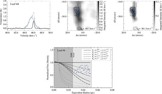
The average spectrum, spatial distribution of integrated N2H+ (1−0) emission, and the radial flux density profile of leaf #4. Note the difference in scaling, which is selected to enhance the features of both components.
The spatially averaged N2H+ (1−0) spectrum taken from the boundary encompassing the leaf is shown in the left-hand panel of Fig. A4. There is a slight asymmetry in the line profile implying the presence of two velocity components. We fitted the spectrum using both one- and two-component models, finding that the latter was more successful in reproducing the observed profile. As in Henshaw et al. (2016a), we base our judgement on: (i) the signal-to-noise level of each component (both of which are >3); (ii) the separation in velocity between the two observed components (which is greater than 0.5 times the FWHM of the narrowest component), which enables one to determine if the two components are distinguishable; (iii) the Akaike information criterion (Akaike 1974), which provides a statistical method of selecting the best model from a number of choices. The centroid velocities of the two components are v0, 1 = 45.69 km s−1 ± 0.03 km s−1 and v0, 2 = 46.14 km s−1 ± 0.01 km s−1. The FWHM line-widths of the two components are Δv1 = 1.50 km s−1 ± 0.05 km s−1 and Δv2 = 0.37 km s−1 ± 0.04 km s−1. As can be seen from the centre and right-hand panels of Fig. A4 the low(er)-velocity component dominates in terms of integrated emission (note the difference in grey-scale between the two plots). We therefore speculate that majority of the mass attributed to leaf #4 is associated with the low-velocity component.
Leaf #5: is situated at {Δα, Δδ} = {2.1 arcsec, −0.9 arcsec}. As with leaf #4, it is elongated, exhibiting the greatest aspect ratio of the identified structures, |$A\!\!{\rm R}$| = 4.73. The figures describing the N2H+ emission associated with leaf #5 can be found in the main text (bottom panels Fig. 3). For reasons discussed in Section 3.2, leaf #5 is rejected from the analysis in Section 4 (other than the mass estimation). However, the centroid velocities and FWHM line-widths associated with the two identified components are v0, 1 = 45.63 km s−1 ± 0.03 km s−1 and v0, 2 = 46.59 km s−1 ± 0.08 km s−1, and Δv1 = 1.10 km s−1 ± 0.07 km s−1 and Δv2 = 0.72 km s−1 ± 0.15 km s−1, respectively.
Leaf #6: is situated at {Δα, Δδ} = { − 0.2 arcsec, 7.5 arcsec}. The leaf boundary has an hourglass-shaped profile, implying the presence of unresolved fragments (see also Fig. A5). The southern half of the hourglass profile is spatially coincident with extended 4.5, 8, and 24 μm emission (note this source appears as a ‘hole’ in the mid-infrared-derived mass surface density map of Kainulainen & Tan 2013; Fig. 1). This leaf was also identified in the Herschel 70 μm images and described as a ‘protostellar massive dense core’ by Nguyen Luong et al. (2011, core #18; their table 1). The mass estimated from the Herschel images is ∼20 ± 9 M⊙, which is consistent with our 3.2 mm continuum-derived masses, Mc ∼ 17 M⊙ and |$M^{\rm b}_{\rm c} \sim 4$| M⊙ (see Section 4). A cursory inspection of the Herschel images show that there may be a secondary 70 μm source within the leaf boundary (i.e. the northern portion of the hourglass). Only when we set |${\rm min\_npix}=15$| (i.e. below the resolution limit of our observations) does the dendrogram algorithm identify the two individual structures. Higher angular resolution observations are required to confirm whether or not this is the case.

The average spectrum, spatial distribution of integrated N2H+ (1−0) emission, and the radial flux density profile of leaf #6. Black Gaussian profiles signify that the continuum flux cannot be unambiguously accredited to a single structure.
Fig. A5 highlights the distribution of N2H+ (1−0) emission associated with this feature. There are two distinct velocity components spatially coincident with leaf #6. The measured centroid velocities and FWHM line-widths are v0, 1 = 45.07 km s−1 ± 0.01 km s−1 and v0, 2 = 47.11 km s−1 ± 0.01 km s−1, and Δv1 = 0.80 km s−1 ± 0.02 km s−1 and Δv2 = 0.95 km s−1 ± 0.03 km s−1, respectively. Since the continuum flux cannot be unambiguously accredited to a single structure, leaf #6 is rejected from the analysis in Section 4 (other than the mass estimation).
Leaf #7: is situated at {Δα, Δδ} = {7.4 arcsec, 22.7 arcsec}, close to the peak in extinction (H6 is located at {Δα, Δδ} = {3.0 arcsec, 21.1 arcsec}; Butler & Tan 2012). Leaf #7 has the smallest aspect ratio of the identified leaves, |$A\!\!{\rm R}$| = 1.46 and an equivalent radius of 3.81 arcsec (corresponding to a physical radius of ∼0.05 pc at a distance of 2900 pc). Although the continuum emission extends both to the south-west and south-east, leaf #7 appears to be monolithic (at the spatial resolution of our PdBI observations). It is dark at 8 and 24 μm, and was identified and classified as a ‘IR-quiet massive dense core’ by Nguyen Luong et al. (2011, core #6; their table 1). The mass estimated from Herschel observations is ∼20 ± 12 M⊙, which is consistent with our continuum-derived masses, Mc ∼ 22 M⊙ and |$M^{\rm b}_{\rm c} \sim 9$| M⊙ (within the factor of 2 uncertainty; see Section 4).
Fig. A6 shows the distribution of N2H+ (1−0) emission associated with leaf #7. The best-fitting solution to the spatially averaged spectrum requires a three-component model. The third component, at ∼47.0 km s−1, is significant to the 5σrms level (a two-component fit increases the residuals by a factor of ≲ 2). The centroid velocities of the measured components are v0, 1 = 45.14 km s−1 ± 0.02 km s−1, v0, 2 = 46.01 km s−1 ± 0.01 km s−1, and v0, 3 = 46.97 km s−1 ± 0.05 km s−1, respectively. The corresponding FWHM line-widths are Δv1 = 0.99 km s−1 ± 0.04 km s−1, Δv2 = 0.50 km s−1 ± 0.03 km s−1, and Δv3 = 0.84 km s−1 ± 0.15 km s−1, respectively. Inspecting the spatial distribution of the emission associated with each component indicates that the low-velocity component dominates over the other two, which are more prominent towards the north and west of the cloud, respectively.
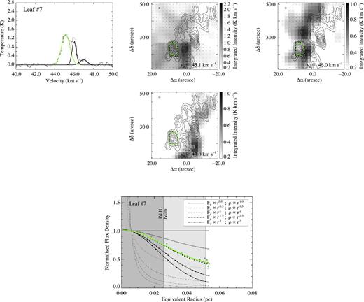
The average spectrum, spatial distribution of integrated N2H+ (1−0) emission, and the radial flux density profile of leaf #7. Note the difference in scaling, which is selected to enhance the features of individual components.
Leaf #8: situated at {Δα, Δδ} = {0.5 arcsec, 23.5 arcsec}, leaf #8 has the smallest projected separation from the H6 extinction peak (located at {Δα, Δδ} = {3.0 arcsec, 21.1 arcsec}; Butler & Tan 2012). Leaf #8 has an aspect ratio of |$A\!\!{\rm R}$| = 1.88 and the continuum emission appears to be singly peaked. Fig. A7 takes a closer look at the distribution of N2H+ emission towards leaf #8. The spectrum indicates the presence of two velocity components. The measured centroid velocities and FWHM line-widths are v0, 1 = 45.17 km s−1 ± 0.01 km s−1 and v0, 2 = 45.83 km s−1 ± 0.02 km s−1, and Δv1 = 0.49 km s−1 ± 0.02 km s−1 and Δv2 = 1.37 km s−1 ± 0.03 km s−1, respectively. We are unable to unambiguously relate either velocity component to the continuum emission. Note that this is different to the cases of leaf #5 and #6, where the continuum emission may be attributed to two independent structures. In this example, we use both measurements of the FWHM line-width for studying the dynamical properties of leaf #8 in Section 4.

The average spectrum, spatial distribution of integrated N2H+ (1−0) emission, and the radial flux density profile of leaf #8. Both Gaussian components appear yellow since although leaf #8 appears to be monolithic in continuum, it cannot be unambiguously linked to either velocity component. Note the difference in scaling, which is selected to enhance the features of both components.
Leaf #9: is situated at {Δα, Δδ} = { − 6.3 arcsec, 28.8 arcsec}. The continuum emission appears monolithic and, under the assumptions made in Section 4, it is the most massive of the identified leaves with Mc ∼ 24 M⊙ and |$M^{\rm b}_{\rm c} \sim 12$| M⊙. Leaf #9 is dark at 70 μm and not identified in Nguyen Luong et al. (2011). The figures describing the N2H+ emission associated with leaf #9 can be found in the main text (top panels Fig. 3). Two spectral components are evident. The measured centroid velocities and FWHM line-widths are v0, 1 = 45.37 km s−1 ± 0.02 km s−1 and v0, 2 = 46.63 km s−1 ± 0.01 km s−1, and Δv1 = 0.79 km s−1 ± 0.04 km s−1 and Δv2 = 0.62 km s−1 ± 0.03 km s−1, respectively. As discussed in Section 3.2, the high-velocity component dominates over the low-velocity counterpart.
Leaf #10: is situated at {Δα, Δδ} = {2.8 arcsec, 34.1 arcsec}. To the north-west of leaf #10 is extended 4.5, 8, and 24 μm emission, implying the presence of an internal heating source. This appears as a ‘hole’ in the mid-infrared-derived mass surface density map of Kainulainen & Tan (2013, Fig. 1). This was identified in the Herschel 70 μm images and described as a ‘protostellar massive dense core’ by Nguyen Luong et al. (2011, core #28; their table 1). The mass estimated from Herschel observations is ∼55 ± 11 M⊙. This is substantially different to our continuum-derived masses, Mc ∼ 8 M⊙ and |$M^{\rm b}_{\rm c} \sim 2$| M⊙. However, we note that leaf #10 is the smallest of the identified leaves, with an angular radius of ∼2 arcsec (corresponding to a physical radius of ∼0.03 pc at a distance of 2900 pc) and that it is slightly offset in position from the location of 4.5, 8, and 24 μm emission. The difference in mass may therefore reflect a difference in source definition.
Fig. A8 shows the distribution of N2H+ (1−0) emission associated with leaf #10. The emission is singly peaked. The measured centroid velocity and FWHM line-width of this component are v0 = 45.79 km s−1 ± 0.01 km s−1 and Δv = 0.98 km s−1 ± 0.02 km s−1, respectively.

The average spectrum, spatial distribution of integrated N2H+ (1−0) emission, and the radial flux density profile of leaf #10.
Leaf #11: is situated at {Δα, Δδ} = { − 12.4 arcsec, 38.7 arcsec}. Although the continuum emission appears monolithic, three spectral components are identified in the spatially averaged spectrum extracted from within the leaf boundary. The centroid velocities of the measured components are v0, 1 = 45.00 km s−1 ± 0.14 km s−1, v0, 2 = 46.05 km s−1 ± 0.06 km s−1, and v0, 3 = 46.75 km s−1 ± 0.03 km s−1, respectively. The corresponding FWHM line-widths are Δv1 = 1.18 km s−1 ± 0.33 km s−1, Δv2 = 0.58 km s−1 ± 0.16 km s−1, and Δv3 = 0.58 km s−1 ± 0.06 km s−1, respectively. Although low in intensity, the low-velocity component is significant to >3 σrms. Inspecting the spatial distribution of integrated emission associated with each component (Fig. A9), it is evident that the high-velocity component dominates over the others.

The average spectrum, spatial distribution of integrated N2H+ (1−0) emission, and the radial flux density profile of leaf #11.
Leaf #12: is situated at {Δα, Δδ} = { − 7.1 arcsec, 42.5 arcsec}. The leaf has an irregular-shaped boundary, with an extension towards the north. This leads to an artificially high aspect ratio of |$A\!\!{\rm R}$| = 2.15. Fig. A10 shows the distribution of N2H+ emission associated with leaf #12. Only one spectral component is identified. The measured centroid velocity and FWHM line-width of this component are v0 = 46.07 km s−1 ± 0.01 km s−1 and Δv = 1.32 km s−1 ± 0.02 km s−1, respectively.

The average spectrum, spatial distribution of integrated N2H+ (1−0) emission, and the radial flux density profile of leaf #12.
Leaf #13: is situated at {Δα, Δδ} = { − 16.9 arcsec, 43.2 arcsec}, and is the northernmost of the identified leaves. It has a high aspect ratio of |$A\!\!{\rm R}$| = 3.55, an irregular-shaped boundary, and the continuum emission has two peaks (see Fig. 2), possibly indicating the presence of unresolved fragments (see also Fig. A11). The top-left panel of Fig. A11 shows the spatially averaged N2H+ spectrum extracted from within the leaf boundary. Three spectral components are evident. The centroid velocities of the measured components are v0, 1 = 45.16 km s−1 ± 0.26 km s−1, v0, 2 = 45.99 km s−1 ± 0.06 km s−1, and v0, 3 = 46.68 km s−1 ± 0.03 km s−1, respectively. The corresponding FWHM line-widths are Δv1 = 0.91 km s−1 ± 0.42 km s−1, Δv2 = 0.71 km s−1 ± 0.22 km s−1, and Δv3 = 0.48 km s−1 ± 0.06 km s−1, respectively. Visual inspection of the spatial distribution of each component reveals that, similar to leaf #5, it appears as though the northern portion of the leaf is associated with one velocity component (∼46 km s−1) whereas the southern portion is associated with another (∼47 km s−1). As a consequence, leaf #13 is rejected analysis in Section 4 (other than the mass estimation).

The average spectrum, spatial distribution of integrated N2H+ (1−0) emission, and the radial flux density profile of leaf #13. Black Gaussian profiles reflect the fact that the continuum flux accredited to leaf #13 cannot be unambiguously attributed to a single structure.
