


Abstract
The shape and diversity of dwarf galaxy rotation curves is at apparent odds with dark matter halos in a Λ Cold Dark Matter (ΛCDM) cosmology. We use mock data from isolated dwarf galaxy simulations to show that this owes to three main effects. Firstly, stellar feedback heats dark matter, leading to a `coreNFW' dark matter density profile with a slowly rising rotation curve. Secondly, if close to a recent starburst, large H i bubbles push the rotation curve out of equilibrium, deforming the rotation curve shape. Thirdly, when galaxies are viewed near face-on, their best fit inclination is biased high. This can lead to a very shallow rotation curve that falsely implies a large dark matter core. All three problems can be avoided, however, by a combination of improved mass models and a careful selection of target galaxies. Fitting our coreNFW model to mock rotation curve data, we show that we can recover the rotation curve shape, dark matter halo mass M200 and concentration parameter c within our quoted uncertainties.
We fit our coreNFW model to real data for four isolated dwarf irregulars, chosen to span a wide range of rotation curve shapes. We obtain an excellent fit for NGC 6822 and WLM, with tight constraints on M200, and c consistent with ΛCDM. However, IC 1613 and DDO 101 give a poor fit. For IC 1613, we show that this owes to disequilibria and its uncertain inclination i; for DDO 101, it owes to its uncertain distance D. If we assume iIC1613 ∼ 15° and DDDO101 ∼ 12 Mpc, consistent with current uncertainties, we are able to fit both galaxies very well. We conclude that ΛCDM appears to give an excellent match to dwarf galaxy rotation curves.
INTRODUCTION
Galaxy rotation curves have provided some of the earliest and most compelling evidence for dark matter in the Universe (Volders 1959; Freeman 1970; Rubin & Ford 1970; Rubin, Ford & Thonnard 1980; van Albada et al. 1985). In all galaxies observed to date, rotation curves fall far more slowly than would be expected from the visible light and gas alone. This is typically taken as evidence for an exotic missing mass component – most likely a new particle that lies beyond the standard model of particle physics1 (e.g. Jungman, Kamionkowski & Griest 1996; Boyarsky, Ruchayskiy & Shaposhnikov 2009; Bertone 2010; Read 2014). However, the nature and properties of such a particle remain unknown.
While rotation curves have long given us evidence for dark matter, there is an enduring puzzle relating to their shape. Almost all rotation curves appear to rise less steeply than is predicted by pure dark matter simulations of structure formation in the standard ΛCDM cosmological model. Such simulations predict central dark matter density profiles that rise as ρ ∼ r−1 (a ‘cusp’; Dubinski & Carlberg 1991; Moore 1994; Navarro, Frenk & White 1996b) in stark contrast with observed rotation curves that favour constant density ‘cores’ (e.g. Flores & Primack 1994; de Blok et al. 2001; de Blok 2010; Oh et al. 2011, 2015; Hague & Wilkinson 2013, 2014; Adams et al. 2014; Oh et al. 2015). This has become known as the cusp-core problem.
One solution to the cusp-core problem is to suggest that there is a problem with the rotation curve data, or with the interpretation of these data (e.g. van den Bosch et al. 2000; Swaters et al. 2003; Hayashi et al. 2004). To explore this, Rhee et al. (2004) used simulated mock rotation curves to test how well they trace the underlying gravitational potential. They focused on three effects: inclination correction; asymmetric drift correction (important if the gas velocity dispersion is a significant fraction of the rotational velocity; see Section 2.1.1); and non-circular motions due to a central bar. They found that the rotation curve is typically biased by about ∼20 per cent due to such effects, though in some extreme cases it can be shifted by up to a factor of 2. Valenzuela et al. (2007) revisited this issue for the specific case of claimed dark matter cores in NGC 3109 and NGC 6822 (the latter of which we will consider here in some detail also). Using numerical simulations as mock data, they performed an end-to-end recovery of the underlying dark matter distribution. They found that if they do not properly correct for thermal and turbulent gas pressure support in the disc (the ‘asymmetric drift’ correction; see Section 2.1.1), then they falsely favour a dark matter core over the correct solution that is cuspy. However, the simulated discs in their study (with a peak rotation velocity of ∼70 km s−1) were rather hot, with a turbulent gas dispersion of σturb ∼ 22 km s−1 (inflated by streaming motions along a central bar), and a gas sound speed of cs ∼ 60 km s−1. NGC 6822, that has a comparable peak rotation velocity, has a measured dispersion of just σgas ∼ 6 km s−1 that is ∼ constant across the disc (Weldrake, de Blok & Walter 2003; and see Section 2.1.1 for a discussion of how σgas relates to σturb and cs). Other galaxies of similar peak rotation velocity are observed to be similarly cold, with σgas in the range 6 < σgas < 15 km s−1 (e.g. Oh et al. 2015). This likely explains why in a later study Kuzio de Naray & Kaufmann (2011) find – seemingly at odds with Valenzuela et al. (2007) – that they are able to successfully disentangle cusps and cores from mock 2D velocity field data, despite ignoring asymmetric drift corrections altogether. Finally, Oh et al. (2011) extract mock rotation curves from dwarf galaxy simulations taken from Governato et al. (2010). They perform and end-to-end analysis similar to that in Valenzuela et al. (2007), finding that they are also able to correctly recover the underlying dark matter distribution.
If dark matter cores are not simply a misinterpretation of observational data, then this opens the door to more exotic explanations. Many authors have suggested that dark matter cores could point to new physics, for example self-interacting or scalar-field dark matter models (e.g. Spergel & Steinhardt 2000; Alcubierre et al. 2002; Magaña & Matos 2012; Zavala, Vogelsberger & Walker 2013; Elbert et al. 2015), or weakly relativistic warm dark matter (e.g. Avila-Reese et al. 2001; Bode, Ostriker & Turok 2001; Strigari, Kaplinghat & Bullock 2007; Boyarsky et al. 2009; Villaescusa-Navarro & Dalal 2011; Macciò et al. 2012). However, before we can conclude that any of these possibilities are favoured by the data, we must first be confident of our model predictions in ΛCDM. It is important to remember that dark matter cusps are a prediction of pure dark matter structure formation simulations. Implicit in these simulations is an assumption that baryons – stars and gas – have little or no impact on the underlying dark matter distribution. There has been a significant debate in the literature about the validity of this approximation. Navarro, Eke & Frenk (1996a) were the first to propose that a central cusp could be transformed to a core by impulsive gas loss driven by supernova explosions. They found that, for reasonable initial conditions and gas collapse factors, the effect of a single burst is very small (see also Gnedin & Zhao 2002). However, Read & Gilmore (2005) showed that multiple repeated bursts can cause this small effect to accumulate, gradually grinding a dark matter cusp down to a core. Such an effect has now been observed in high resolution hydrodynamic simulations that resolve the interstellar medium (e.g. Mashchenko, Wadsley & Couchman 2008; Governato et al. 2010; Teyssier et al. 2013; Di Cintio et al. 2014; Oñorbe et al. 2015; Trujillo-Gomez et al. 2015; Read, Agertz & Collins 2016; and for a review see Pontzen & Governato 2014). The physics of such cusp-core transformations is now well understood (Pontzen & Governato 2012; Pontzen et al. 2015), while there is mounting observational evidence for the bursty star formation that is required to drive the process (e.g. Leaman et al. 2012; Weisz et al. 2012; Teyssier et al. 2013; Kauffmann 2014; McQuinn et al. 2015; El-Badry et al. 2016; Read et al. 2016).
The above progress suggests that cusp-core transformations driven by stellar feedback likely explain the observed shallow rise seen in many dwarf galaxy rotation curves. However, recently a new problem has emerged: the diversity of dwarf galaxy rotation curves. Oman et al. (2015) compared dwarfs from recent cosmological hydrodynamic simulations with a wide array of observed dwarf galaxy rotation curves, including those from the THINGS and Little THINGS surveys (de Blok et al. 2008; Oh et al. 2011; Hunter et al. 2012; Oh et al. 2015; we refer the reader to Oman et al. 2015 for a full list of the data they use). They found that the data show a wide variety of rotation curve shapes at fixed peak rotation velocity, in stark contrast with their simulations that show remarkably little scatter. In particular, some galaxies exhibit an extremely shallow rise that appears to imply truly massive dark matter cores ≳ 4 kpc – far larger than the ≲ 1 kpc cores predicted by recent simulations. Oman et al. (2016) suggest that this could owe to systematic inclination and/or distance errors in the rotation curve reconstruction, but it remains to be seen whether such large systematic errors are plausible. By contrast, Brook (2015) suggest that the diversity could owe to the expected halo-to-halo scatter in ΛCDM that is amplified by dark matter cusp-core transformations.
In this paper, we use two recent high resolution simulations of isolated dwarf galaxies (of mass M200 = 5 × 10⁸ M⊙ and 109 M⊙) to shed light on both the shape and diversity of dwarf galaxy rotation curves. Our simulations reach a minimum cell size of 4 pc, allowing us to resolve the effect of individual supernova explosions. At this resolution, we become insensitive to our ‘sub-grid’ numerical parameters, making the simulations substantially more predictive (Read et al. 2016, hereafter R16). In R16, we showed that our simulated dwarfs give an excellent match to the photometric light profiles; star formation histories; metallicity distribution functions; and star/gas kinematics of low mass isolated dwarfs in the field without any fine-tuning of the model parameters. Here, we use these simulations to create dynamically realistic mock rotation curve data. We start by assuming that we can reliably correct for inclination and asymmetric drift, looking first at the effect of H i bubbles driven by stellar feedback on the rotation curve, and the importance of dark matter cusp-core transformations. We then consider how well we can reconstruct the inclination and asymmetric drift corrected rotation curve from mock inclined H i data cubes. In all cases, we fit our mock rotation curves using the emceepython package of Foreman-Mackey et al. (2013) to test how well we can recover the halo mass M200 and concentration parameter c (see equation 1). In performing these fits, we make use of our new coreNFW dark matter halo profile that accounts for cusp-core transformations driven by stellar feedback (Section 4.1; and R16). Finally, we apply our rotation curve fitting method to real data for four isolated dwarf galaxies: NGC 6822; WLM; IC 1613; and DDO 101, chosen to span a range of interesting rotation curve shapes. Using the insight gained from our mock data analysis, we discuss why we obtain an excellent fit for two of these galaxies (NGC 6822 and WLM) but seemingly not for the other two (IC 1613 and DDO 101).
This paper is organized as follows. In Section 2, we briefly review the numerical simulations (these are discussed in more detail in R16). In Section 3, we describe our data compilation for NGC 6822, WLM and IC 1613, and we briefly describe the 3DBarolo method for extracting rotation curves from these data (Di Teodoro & Fraternali 2015). In Section 4, we describe our rotation curve fitting method that makes use of our coreNFW profile and the emcee code. In Section 5.1, we apply this method to our mock data. In Section 5.4, we apply our method to real data for four isolated dwarf galaxies: NGC 6822; WLM; IC 1613; and DDO 101. Finally, in Section 6 we present our conclusions.
THE SIMULATIONS
We consider here two of the simulations from R16 set up as above with masses M200 = 5 × 10⁸ and 109 M⊙, labelled M5e8c25_2e6 and M9c22_4e6, respectively. They both have a dark matter particle resolution of mdm = 250 M⊙; a finest grid cell size gas resolution of Δx ≈ 4 pc; and a stellar sampling mass of m* = 300 M⊙ (see e.g. Dubois & Teyssier 2008). Note that the virial masses M200 refer to the total mass in gas plus dark matter. The dark matter halo masses for these models are slightly lower: M200, DM = M200(1 − fb) = 0.85M200 (R16).
The simulations were evolved for 14 Gyr each, using the Adaptive Mesh Refinement (AMR) code RAMSES (Teyssier 2002) with cooling, star formation and feedback physics prescriptions as described in detail in Agertz et al. (2013); Agertz & Kravtsov (2015) and R16.
The true gas spatial resolution of the simulations in R16 is somewhat larger than the minimum cell size. However, even using the Truelove et al. (1997) criteria of ∼4Δx ≈ 16 pc, the resolution scale is substantially smaller than the projected half stellar mass radii of the simulated galaxies (R1/2 ∼ 200–500 pc). The simulations are also robust to spurious two-body relaxation over a Hubble time (e.g. Power et al. 2003) on scales ≳ 40 pc (see R16, appendix A1).
The key result from these R16 simulations was that star formation over a Hubble time transformed the initial NFW dark matter distribution into a ‘coreNFW’ profile that has ∼ constant density within R1/2 (see Section 4.1 for a complete description of the coreNFW profile). In R16, we showed that this result is robust to order-of-magnitude changes in the numerical ‘sub-grid’ physics parameters and/or initial conditions. As a result, we claimed that the coreNFW profile is the correct prediction for a ΛCDM cosmology (with baryons) on mass scales 108 ≲ M200/M⊙ ≲ 1010, at least to within a factor of ∼2 scatter in the coreNFW profile parameters2. This robustness is a direct result of the numerical resolution in R16 that has two key effects: (i) we correctly capture the momentum injection into the interstellar medium (ISM) generated by expanding bubbles of shock heated gas (e.g. Kimm et al. 2015); and (ii) star formation becomes self-regulated by stellar feedback (e.g. Kravtsov 2003; Saitoh et al. 2008; Hopkins, Quataert & Murray 2011; Agertz et al. 2013; Hopkins, Narayanan & Murray 2013).
Extracting the rotation curves
We analyse the 109 M⊙ simulation at several different times throughout its starburst cycle, focusing on a ‘quiescent’ phase, a ‘starburst’ phase and a ‘post-starburst’ phase (see Fig. 1). We analyse the 5 × 10⁸ M⊙ dwarf at a simulation time of 14 Gyr, when it is quiescent with little recent star formation (see R16). The simulations were rotated and centred such that the gas discs are aligned with the x − y plane. We then define the gas as being ‘H i’ if it has temperature T < 104 K. Under collisional ionization equilibrium, this is the temperature at which the ionization fraction is unity. We find that cutting instead on T = 2 × 10⁴ K (where the ionization fraction is <10 per cent) makes very little difference to our results.
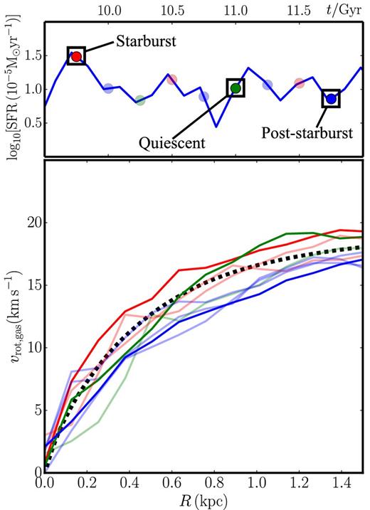
Asymmetric drift corrected rotation curves (cf. Section 2.1.1) for our M200 = 109 M⊙ simulation at nine regularly spaced time intervals over the starburst cycle (bottom panel). The upper panel shows the star formation rate as a function of time; the lower panel shows the gas rotation curves at the times marked by the circles in the upper panel. The red circles correspond to a ‘starburst’ phase in the cycle; the blue to ‘post-starburst’; and the green to a more ‘quiescent’ phase. In Section 5.1.2, we will fit models to the three times marked by the black squares. Notice that there is a general trend that when the star formation rate is increasing, the rotation curve amplitude is higher (red), while when it is decreasing, the rotation curve amplitude is lower (blue). The black dashed line marks the true rotation curve as calculated from the gravitational potential.
Asymmetric drift correction
We discuss more sophisticated asymmetric drift corrections in Appendix A where we explore the effect of a wide range of Σgas profiles on WLM's rotation curve. The differences in both the rotation curve and its implied M200 and c lie in every case within our quoted 1σ uncertainties.
We added Gaussian velocity errors of fixed variance σgas, err = 1 km s−1 to the above rotation curves.
Mock H i data cubes
In Section 5.3, we consider how well we can reconstruct the rotation curve from mock inclined H i data cubes. We generate these by slicing the data in velocity channels of width 1 km s−1 at a spatial resolution of 50 pc for a range of inclination angles: i = 15°, 30°, 45°, 60°, 75°. We do not explicitly add any broadening due to thermal or turbulent pressure support as our primary goal with these data cubes is to test how well we can recover inclination. To simulate real observations, we added random Gaussian noise to these mock data and then applied both a 2D spatial and a 1D velocity (Hanning) smoothing. In this way, we obtained a simulated observation of the mock data cubes with an instrumental beam of 20 arcsec and with a noise per channel of ∼0.027 M⊙ pc−2, that is the typical value found in the Little THINGS data cubes at this resolution (Hunter et al. 2012).
Our method for extracting rotation curves from these H i data cubes is described in Section 3.1. Once extracted, we applied an asymmetric drift correction as in Section 2.1.1 to these rotation curves.
THE DATA
We study four dwarf galaxies with excellent literature data, chosen to span a wide range of rotation curve shapes: NGC 6822; WLM; IC 1613; and DDO 101. The data are summarized in Table 1. We briefly discuss each galaxy in turn, next. Our method for extracting rotation curves from H i data cubes is described in Section 3.1.
Four isolated dwarf irregular galaxies with excellent literature data, chosen to span a range of rotation curve shapes. The first column gives the galaxy name. Columns 2–7 give the data for that galaxy: the peak asymmetric drift corrected rotation curve velocity vmax; the inclination angle i in degrees (with formal 1σ errors; see Section 5.3 for a discussion of the validity of these); the distance to the galaxy D; the stellar mass, with errors, M*; the total gas mass Mgas; and the exponential stellar and gas disc scale lengths R* and Rgas, respectively. Column 8 gives the radial range used in the fit to the rotation curve [Rmin, Rmax] (‘−’ indicates that Rmax is set to the outermost data point). Columns 9–10 give the marginalized dark matter halo parameters: the virial mass M200 and concentration parameter c, with 68 per cent confidence intervals. Column 11 gives the reduced |$\chi ^2_{\rm red}$| of the fit (we discuss how to interpret these |$\chi ^2_{\rm red}$| values in Section 5.4). Finally, column 12 gives the data references for that galaxy as follows: 1: Barnard (1884); 2: Weldrake et al. (2003); 3: Zhang et al. (2012); 4: Górski et al. (2011); 5: Leaman et al. (2012); 6: Oh et al. (2015). For IC 1613, there are two entries corresponding to different inclination angles i (see Section 5.4.2), while for DDO 101 there are three corresponding to different distances D (see Section 5.4.3).
| Galaxy | |$\boldsymbol v_{\rm max}$| | |$\boldsymbol i$| | D | M* | Mgas | R* | Rgas | [Rmin, Rmax] | M200 | c | |$\boldsymbol {\chi ^2_{\rm red}}$| | Refs |
|---|---|---|---|---|---|---|---|---|---|---|---|---|
| (km s−1) | (°) | (kpc) | (M⊙) | (M⊙) | (kpc) | (kpc) | (kpc) | (M⊙) | ||||
| NGC 6822 | 55 | 65 (inner); 75 (outer) | 490 ± 40 | 7.63 ± 1.9 × 10⁷ | 17.4 × 10⁷ | 0.68 | 1.94 | [2.5, −] | |$2^{+0.2}_{-0.3} \times 10^{10}$| | |$15.1^{+1.8}_{-0.8}$| | 0.37 | 1,2,3 |
| WLM | 39 | 74 ± 2.3 | 985 ± 33 | 1.62 ± 0.4 × 10⁷ | 7.9 × 10⁷ | 0.75 | 1.04 | [0, −] | |$8.3_{-2.2}^{+2.1}\times 10^9$| | |$17^{+3.9}_{-2.2}$| | 0.27 | 3,4,5,6 |
| IC 1613 | 20 | 39.4 ± 2.29 | 740 ± 10 | 1.5 ± 0.5 × 10⁷ | 8 × 10⁷ | 0.65 | 1.29 | [1.9, −] | |$4.7^{+1.2}_{-0.98} \times 10^8$| | |$21.8_{-5.4}^{+5.3}$| | 0.13 | 3,6 |
| 41 | 15 | [1.9, −] | |$7.75_{-2}^{+4}\times 10^9$| | |$21.7_{-5.5}^{+5.5}$| | 0.32 | |||||||
| DDO 101 | 65 | 52.4 ± 1.7 | 6,400 | 6.54 ± 1 × 10⁷ | 3.48 × 10⁷ | 0.58 | 1.01 | [0, −] | |$5.2^{+0.6}_{-0.4} \times 10^{10}$| | |$28.9_{-1.3}^{+0.6}$| | 7.2 | 3,6 |
| 12,900 | 26.6 ± 4 × 10⁷ | 14.13 × 10⁷ | 1.16 | 2.03 | [0, −] | |$3.0^{+0.4}_{-0.2} \times 10^{10}$| | |$28.3_{-2.2}^{+1.1}$| | 1.92 | ||||
| 16,000 | 40.9 ± 6 × 10⁷ | 21.75 × 10⁷ | 1.45 | 2.5 | [0, −] | |$2.7^{+0.5}_{-0.2} \times 10^{10}$| | |$27.6_{-3.3}^{+1.6}$| | 1.1 |
NGC 6822: NGC 6822 was first discovered by Barnard (1884). It is one of the closest isolated dwarf irregulars known, lying some D = 490 ± 40 kpc from the Milky Way (Mateo 1998). For this reason, it has a wealth of excellent data. In particular, its high resolution rotation curve extends to an impressive ∼5 kpc from the galactic centre (Weldrake et al. 2003). It has a relatively smooth H i gas distribution, with the exception of a large H i hole of size 1.4 - 2 kpc (de Blok & Walter 2000, and see Fig. 5 upper left panel). Several theories have been put forward for the origin of this and similar holes in dwarf irregular galaxies. One possibility is that the hole formed as a result of a merger/interaction with a high velocity gas cloud or smaller companion galaxy (e.g. Tenorio-Tagle et al. 1987; Bekki & Chiba 2006); another is that the hole results from gravitational instability in the disc (e.g. Wada, Spaans & Kim 2000, and for a review see Tenorio-Tagle & Bodenheimer 1988). However, it is now widely accepted that most of these holes, including the one in NGC 6822, owe to stellar feedback (Bruhweiler et al. 1980; Sánchez-Salcedo 2001; Cannon et al. 2012; Kannan et al. 2012). Cannon et al. (2012) show that there is sufficient energy from star formation to create the hole in NGC 6822 and they estimate an age of >500 Myr, consistent with its low/zero expansion velocity. Interestingly, the hole coincides with a notable dip in the rotation curve (see Fig. 5, upper row), a correspondence that we discuss further in Section 5.3. However, the rotation curve within ∼2.5 kpc is also affected by the possible presence of a stellar bar or a misaligned stellar component (Demers, Battinelli & Kunkel 2006) making such a correspondence possibly coincidental. NGC 6822 appears to be at a relatively quiescent moment in its history, having formed stars over the past 0.1 Gyr at about half of its mean rate over a Hubble time: SFR0.1 Gyr/〈SFR〉 = 0.51 ± 0.14 (Zhang et al. 2012).
WLM: WLM was first discovered by Wolf (1909) and later rediscovered by Lundmark and Melotte (1926) – hence the name WLM. It lies some D ∼ 1 Mpc from both the Milky Way and Andromeda (Górski, Pietrzyński & Gieren 2011) and so is remarkably isolated. It has excellent H i data, photometry and stellar kinematics (e.g. Leaman et al. 2012; Zhang et al. 2012; Oh et al. 2015). Its H i distribution is smooth, apart from the presence of a small H i hole of size ∼0.46 kpc (Kepley et al. 2007, and see Fig. 5 second row, leftmost panel). Its hole has no measured expansion velocity and so, similarly to the H i hole in NGC 6822, is likely quite old. There is no evidence for significant non-circular motions in the gas and its rotation curve is quite smooth (e.g. Oh et al. 2015). WLM appears to be relatively quiescent at the present time, showing substantially lower than average star formation over the past 0.1 Gyr: SFR0.1 Gyr/〈SFR〉 = 0.43 ± 0.11 (Zhang et al. 2012).
IC 1613: IC 1613 was first discovered by Baade (1929). It is a near face-on dwarf irregular on the edge of the Local Group, some ∼740 kpc away (Scowcroft et al. 2013). It has been mass modelled numerous times in the literature before (e.g. Lake & Skillman 1989; Oh et al. 2015), while many authors have noted the clumpy nature of its ISM, with substantial H i bubbles and shells (Lozinskaya 2002; Silich et al. 2006). The most prominent of these has a size of ∼1 kpc and a large expansion velocity of ∼25 km s−1. Its rotation curve also has a strange morphology, with two notable dips (see Fig. 5, second row, second panel). We discuss this further in Section 5. IC 1613 formed stars over the past 0.1 Gyr at a rate close to the mean over a Hubble time: SFR0.1 Gyr/〈SFR〉 = 0.81 ± 0.25 (Zhang et al. 2012). This is substantially higher than WLM, DDO 101 and NGC 6822 and consistent with the violent appearance of its H i column density map.
DDO 101: DDO 101 (also called UGC 6900) is substantially more distant than the other galaxies. Its distance is typically assumed to be DDDO101 = 6.4 Mpc (e.g. Oh et al. 2015), however the uncertainties on DDDO101 are very large. It it too far away for an accurate tip-of-the-red-giant-branch or Cepheid distance measurement, and so its distance must be determined instead from matching its peak rotation velocity to the Tully–Fisher relation (Tully & Fisher 1977). This introduces large uncertainties both because of the intrinsic scatter in the Tully–Fisher relation, particularly at low peak rotation velocity (e.g Meyer et al. 2016), but also because its measured peak rotation velocity is only a lower bound on the true maximum. According to the NASA/IPAC Extragalactic Database (NED), its distance could lie in the range 6 < DDDO101/Mpc < 16, while its cosmological ‘Hubble flow’ distance is 12.9 Mpc (assuming the latest cosmological parameters from Planck Collaboration XVI 2014). The earliest literature on DDO 101 that we could find are its listing in the Nilson (1973) and Tully & Fisher (1988) catalogues. It has had its neutral hydrogen mapped by Schneider et al. (1990) and most recently by Little THINGS (Oh et al. 2015). Its star formation rate over the past 0.1 Gyr is substantially lower than its average over a Hubble time, indicating that it is not currently starbursting (Zhang et al. 2012 estimate SFR0.1 Gyr/〈SFR〉 = 0.08 ± 0.02). DDO 101 is one of the few galaxies in the Little THINGS survey that has a steeply rising rotation curve and this is our motivation for including it here. Oh et al. (2015) note that as a result, it is one of the few galaxies that appears to be well fit by an NFW profile.
Extracting rotation curves from H i data cubes
We derived the rotation curves from the H i data cubes using the publicly available software 3DBarolo3 (Di Teodoro & Fraternali 2015). 3DBarolo fits tilted-ring models directly to the data cube by building artificial 3D data and minimizing the residuals, without explicitly extracting velocity fields. This ensures full control of the observational effects and in particular a proper account of beam smearing that can strongly affect the derivation of the rotation velocities in the inner regions of dwarf galaxies (see e.g. Swaters, Sancisi & van der Hulst 1997). 3DBarolo fits up to nine parameters for each ring in which the galaxy is decomposed, namely: central coordinates; systemic velocity; inclination (i); position angle (p.a.); H i density; H i thickness; rotation velocity (vrot); and velocity dispersion (|$\sigma _{\rm H\,\small {i}}$|).
In order to obtain a good fit of the kinematics, it is important to start with reasonable initial guesses for the inclination i and the position angle p.a. We use 3DBarolo to estimate these initial guesses by fitting the total H i map. We then estimated rotation and dispersion in two stages. First 3DBarolo makes a fit leaving the four parameters free. Then it fixes the geometrical parameters, regularising them with a polynomial and performing a new fit of vrot(R) and |$\sigma _{\rm H\,\small {i}}(R)$| alone.
The H i data for WLM, IC 1613 and DDO 101 were obtained from the publicly available archive of the Little THINGS survey4, while the H i data cube of NGC 6822 was kindly provided to us by Erwin de Blok. For WLM and IC 1613, we used natural weighted data smoothed to a resolution of 25 arcsec that represents a good compromise between the number of resolution elements and the enhancement of the galaxy signal. The extent of DDO 101 on the sky is very small so we used the robust weighted data at the original resolution of about 8 arcsec without further smoothing. Finally, for NGC 6822 we smoothed the original cube from a resolution of 42x12 to 43×30 arcsec.
Except for the case of NGC 6822, the data did not show any clear radial trends in the geometrical parameters, so we fitted them with a constant value; we report the best-fitting values of i with formal error bars in Table 1. For NGC 6822, we found that the inclination rises from about 65° in the centre to 70° in outskirts.
The final rotation curves were corrected for asymmetric drift (Section 2.1.1), fitting the |$\Sigma _{\rm g}\sigma ^2_{\rm g}$| data with a functional form (see Appendix A for further details and tests of our asymmetric drift correction).
THE ROTATION CURVE FITTING METHOD
The mass model
From equation (22), we see that even at R = 2R1/2, the coreNFW rotation curve has ∼90 per cent of the amplitude of the equivalent NFW rotation curve. Since for our simulations, the dark matter dominates the total enclosed mass at all radii, the total rotation curve vc(R) ≃ vdm(R). Thus, the dark matter cores in R16, although visually of a size ∼R1/2, will affect the full rotation curve out to ∼2R1/2.
Fitting the mass model to data and our choice of priors
We fit the above mass model to the data using the emcee affine invariant Markov Chain Monte Carlo (MCMC) sampler from Foreman-Mackey et al. (2013). We assume uncorrelated Gaussian errors such that the Likelihood function is given by |$\mathcal {L} = \exp (-\chi ^2/2)$|. We use 100 walkers, each generating 1500 models and we throw out the first half of these as a conservative ‘burn in’ criteria. We explicitly checked that our results are converged by running more models and examining walker convergence. All parameters were held fixed except for the dark matter virial mass M200; the concentration parameter c; and the total stellar mass M*. We assume a flat logarithmic prior on M200 of 8 < log10[M200/M⊙] < 11; a flat linear prior on c of 14 < c < 30 and a flat linear prior on M* over the range given by stellar population synthesis modelling, as reported in Table 1. For the mock simulation data and the real data, we assume an error on M* of 25 per cent unless a larger error than this is reported in the literature (e.g. Zhang et al. 2012; Oh et al. 2015). The generous prior range on c is set by the cosmic mean redshift z = 0 expectation value of c at the extremities of the prior on M200 (Macciò et al. 2007); we explore our sensitivity to this choice of prior in Appendix D. For each galaxy, we fit data over a range [Rmin, Rmax] as reported in Table 1. Where we write ‘–’ for Rmax, this means that Rmax is set by the outer edge of the rotation curve data.
RESULTS
Fitting models to ideal mock data
In this section, we first consider mock data that are ‘as good as it gets’; that is, we assume that we can perfectly inclination and asymmetric drift correct the rotation curves, as described in Section 2. We then explore how well we can recover the dark matter halo mass M200 and concentration parameter c when fitting the mass model described in Section 4 to these mock data. (We will explore how well we can inclination and asymmetric drift correct mock H i data cubes in Section 5.3.)
Starburst-induced variance in the rotation curve
Before fitting the mock rotation curves, let us first take a look at the time evolution of the mock galaxy rotation curve through the starburst cycle. In Fig. 1, we show asymmetric drift corrected rotation curves (cf. Section 2.1.1) for our M200 = 109 M⊙ simulation at 9 regularly spaced time intervals over the starburst cycle (bottom panel). The upper panel shows the star formation rate as a function of time; the lower panel shows the gas rotation curves at the times marked by the circles in the upper panel. The red circles correspond to a ‘starburst’ phase in the cycle; the blue to ‘post-starburst’; and the green to a more ‘quiescent’ phase. In Section 5.1.2, we will fit models to the three times marked by the black squares.
Notice that there is a general trend that when the star formation rate is increasing, the rotation curve amplitude is higher (red), while when it is decreasing, the rotation curve amplitude is lower (blue). At quiescence, the rotation curve lies in between these extremes (green), in good agreement with the true rotation curve7 (black dashed line). Such a movement in the asymmetric drift corrected rotation curve occurs continuously throughout the starburst cycle. If real galaxies behave similarly to this, then we expect them to be equally often in all three phases, though the most extreme departures from quiescence will be more rare. We now consider how such a variation in the rotation curve affects rotation curve modelling.
Fitting mock rotation curves through the starburst cycle
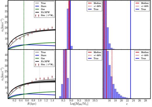
In Fig. 2, we fit the model described in Section 4 to our mock rotation curve data. We analyse the 109 M⊙ simulation at three times, marked as ‘quiescent’; ‘starburst’ and ‘post-starburst’ on Fig. 1 (top three rows). We also analyse the 5 × 10⁸ M⊙ simulation at a simulation time of 14 Gyr (bottom row). From left to right, the columns show the gas density viewed face-on; the mean vertical velocity of the gas for this same face-on view; the fitted asymmetric drift corrected rotation curve; and the resultant constraints on the dark matter virial mass M200 and concentration parameter c. On the rotation curve plots, we mark the projected half stellar mass radius R1/2 by the vertical green dashed line; the mock rotation curve data with errors (red data points); the true model rotation curve (black dashed line); the star (blue) and gas (green) contribution to the rotation curve; and the median (black); 68 per cent (dark grey) and 95 per cent (light grey) confidence intervals of our fitted model rotation curves. The magenta line and dark/light magenta bands show what the median, 68 per cent and 95 per cent confidence intervals of our model rotation curves would look like if we switched off cusp-core transformations (i.e. if we apply the NFW profiles that correspond to our fitted coreNFW profiles). The fourth and fifth panels from the left show histograms of our recovered M200 and c; the true answers are marked by the vertical blue lines.
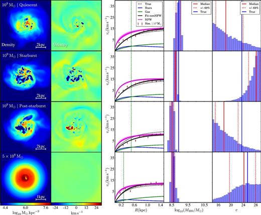
Fitting the model described in Section 4 to ideal mock rotation curve data. From left to right, the columns show the gas density viewed face-on; the mean vertical velocity of the gas for this same face-on view; the fitted asymmetric drift corrected rotation curve; and the resultant constraints on the dark matter virial mass M200 and concentration parameter c. On the rotation curve plots, we mark the projected half stellar mass radius R1/2 by the vertical green dashed line; the mock rotation curve data with errors (red data points); the true model rotation curve (black dashed line); the star (blue) and gas (green) contribution to the rotation curve; and the median (black); 68 per cent (dark grey) and 95 per cent (light grey) confidence intervals of our fitted model rotation curves. The magenta line and dark/light magenta bands show what the median, 68 per cent and 95 per cent confidence intervals of our model rotation curves would look like if we switched off cusp-core transformations (i.e. if we apply the NFW profiles that correspond to our fitted coreNFW profiles). The fourth and fifth panels from the left show histograms of our recovered M200 and c; the true answers are marked by the vertical blue lines.
First, notice that in all simulations there are H i bubbles being blown through the disc by stellar feedback (Fig. 2, leftmost panels). These typically reach a velocity ∼30 km s−1 (Fig. 2, second column) in excellent agreement with data for real isolated dwarfs (see Table 1 and Section 5.4). The ‘quiescent’ mock (top row) shows very little activity, resulting in a rotation curve that is closely matched to the underlying circular speed curve vrot, gas ∼ vc. Our fit returns a minimum reduced |$\chi ^2_{\rm red} = 1.79$|, corresponding to a good representation of the data. We obtain an excellent recovery of M200 within our quoted uncertainties (compare the vertical blue line with the histogram in the fourth panel from left, upper row). However, it is substantially harder to recover the halo concentration c and the constraints are much poorer (see rightmost panel, upper row).
The second row of Fig. 2 shows our results for the ‘starburst’ mock. At this output time, the gas is in a highly turbulent state, and features many fast-moving H i bubbles of size ∼0.5–1 kpc and expansion velocity ∼30 km s−1. This causes a substantially steeper rise in the inner rotation curve. Interestingly, our emcee fit skirts between the inner and outer rotation curve data points, leading to a highly biased concentration parameter c that pushes on our prior, and an underestimate of M200. The minimum reduced |$\chi ^2_{\rm red} = 2.4$| is noticeably poorer than for the quiescent case. This is because the rotation curve within R1/2 (vertical green dashed line) rises more steeply than our model ensemble. If we restrict our fit to R < R1/2, then we find that we systematically overestimate M200, as might naively be expected for a rotation curve that rises too steeply.
The third row of Fig. 2 shows our results for the ‘post-starburst’ mock. Like the starburst mock, it is similarly out of equilibrium, with substantial H i bubbles. However, instead of many smaller H i bubbles, these have agglomerated into one enormous outflow. The rotation curve is now systematically shallower than in quiescence, even out to the outermost rotation curve data point at R = 1.5 kpc. When fitting our mass model to these mock data, this leads to an underestimate of M200 by ∼ half a dex. However, the minimum reduced |$\chi ^2_{\rm red} = 1.0$| indicates an excellent fit. This demonstrates that we cannot rely on |$\chi ^2_{\rm red}$| alone as an indicator that the rotation curve is out of equilibrium. Instead, we must look for evidence of fast-moving and substantial H i bubbles in the H i velocity field, with associated star formation activity over the past ∼100 Myr (see Fig. 1).
The importance of cusp-core transformations
In the third column of Fig. 2, we illustrate the importance of properly accounting for cusp-core transformations driven by stellar feedback. The magenta bands show the rotation curves that would arise if we ‘undid’ the cusp-core transforms (i.e. if we insert the best-fitting coreNFW profile parameters into the NFW profile and calculate the resulting rotation curves). Notice that these all rise substantially more steeply than the data, as expected. If we fit NFW profiles to these mock data instead of coreNFW, we become biased towards extremely low concentration parameters inconsistent with cosmological expectations. The mass M200 is, however, still correctly recovered so long as the rotation curve data extend far enough out. If the rotation curve does not extend to the point where it becomes flat, then when fitting NFW instead of coreNFW, we become biased also towards low M200 (see Appendix B).
Fitting rotation curves at the edge of galaxy formation
In the bottom row of Fig. 2, we fit the rotation curve for our lower mass mock with M200 = 5 × 10⁸ M⊙. Despite having just about the lowest mass possible for a galaxy that can continue to form stars for a Hubble time (see discussion in R16), our mock displays a rather smooth rotation curve that – once corrected for asymmetric drift – corresponds well with the underlying potential. As a result, we obtain an excellent recovery of M200. This suggests that we should be able to recover M200 and c from even very tiny dwarf irregulars like LeoT or Aquarius (e.g. Young et al. 2003; Irwin et al. 2007; Ryan-Weber et al. 2008).
The effect of the starburst cycle on the stellar kinematics
There are now a subset of isolated dwarfs with stellar kinematic data (e.g. Adams et al. 2014; Kirby et al. 2014). For this reason, it is interesting to ask whether the stars are also pushed out of equilibrium by stellar feedback. In Fig. 3, we show the radial (blue) and angular (green, ϕ; red, θ) components of the stellar velocity dispersion in spherical polar coordinates (σr, ϕ, θ; dashed lines) and the mean streaming velocity in these coordinates (〈vr, ϕ, θ〉; solid lines), as indicated in the legend, for our M200 = 109 M⊙ mock in quiescence (left) and post-starburst (right). Notice that the two plots are very similar. In both cases, dispersion dominates over rotation inside R1/2 (vertical green line), while the opposite is true beyond R1/2. However, while the two cases are remarkably similar, the post-starburst system has a slightly larger projected half stellar mass radius while its dispersions rise slightly more slowly and with lower radial anisotropy. Using an analysis similar to that presented in R16, we have verified that these small changes are not sufficient to substantially bias Jeans modelling of the stars by more than ∼1 km s−1 (assuming perfect data).
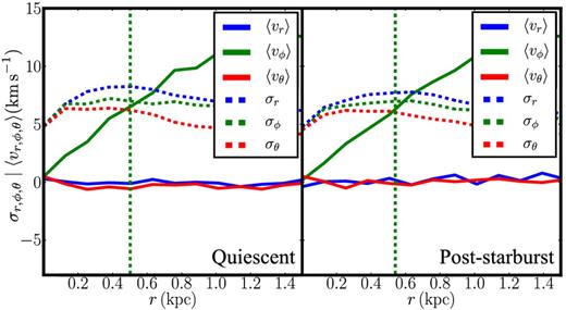
The radial (blue) and angular (green, ϕ; red, θ) components of the stellar velocity dispersion in spherical polar coordinates (σr, ϕ, θ; dashed lines) and the mean streaming velocity in these coordinates (〈vr, ϕ, θ〉; solid lines), as indicated in the legend, for our M200 = 109 M⊙ mock in quiescence (left) and post-starburst (right). The vertical green dashed line marks the projected half stellar mass radius R1/2 in both cases.
We may be tempted to conclude from the above analysis that stars are a more robust probe of the underlying potential than the gas. However, as emphasized in R16, the stars give a reliable estimate of the mass only within ∼R1/2 (e.g. Walker et al. 2009; Wolf et al. 2010; Campbell et al. 2016). Yet this is precisely where stellar feedback affects the gravitational potential (R16; and see Oñorbe et al. 2015), making it challenging to obtain a robust estimate of M200. By contrast, H i gas traces the gravitational potential much further out, often to the point where the rotation curve becomes flat. Thus, stellar kinematic and H i data remain complementary. We defer a full analysis of the efficacy of combined stellar and H i kinematics to future work.
Deprojecting mock H i data cubes: how well can we recover the inclination?
In this section, we now consider how well we can recover the rotation curve from mock H i data cubes. The mock data are described in Section 2.1.2, while extracting rotation curves from these using 3DBarolo is described in Section 3.1. The results for the quiescent and starburst mocks are shown in Fig. 4. The top left panel shows the surface density of the starburst mock viewed at an inclination of itrue = 15°. The red circle marks an ellipse showing this correct inclination (ifit = itrue = 15°); the orange dashed circle shows instead ifit = 38°. The bottom left panel plots the true inclination itrue versus the recovered inclination ifit from the 3DBarolo code (see Section 3.1) for the ‘quiescent’ mock (blue) and the ‘starburst mock’ (red) at inclinations itrue = 15°, 30°, 45°, 60°, 75°. The error bars mark the 68 per cent confidence intervals generated from 100 different simulated observations of the same data cube (recall that these are different because each realization has different Gaussian random noise added to it; see Section 2.1.2). The top right two panels show the recovered rotation curve from 3DBarolo for ifit = itrue = 15°, and the resulting histogram of M200 from our model fits (the lines and symbols are as in Fig. 2). The bottom right two panels show the same for ifit = 38°, corresponding to a large systematic overestimate of the inclination angle.
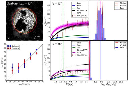
Recovering the inclination and rotation curve from mock H i data cubes. The top left panel shows the surface density of our ‘starburst’ mock dwarf viewed at an inclination of itrue = 15°. The red circle marks an ellipse showing this correct inclination (ifit = itrue = 15°); the orange dashed circle shows instead ifit = 38°. The bottom left panel plots the true inclination itrue versus the recovered inclination ifit from the 3DBarolo code (see Section 3.1) for the ‘quiescent’ mock (blue) and the ‘starburst’ mock (red) at inclinations itrue = 15°, 30°, 45°, 60°, 75°. The error bars mark the 68 per cent confidence intervals generated from 100 different simulated observations of the same data cube (see text for details). The top right two panels show the recovered rotation curve from 3DBarolo for ifit = itrue = 15°, and the resulting histogram of M200 from our model fits (the lines and symbols are as in Fig. 2). The bottom right two panels show the same for ifit = 38°, corresponding to a large systematic overestimate of the inclination angle. This leads to an artificially shallow rotation curve, with an amplitude that is suppressed by a factor sin (itrue)/sin (ifit) ∼ 0.4.
Notice from the bottom left plot of ifit versus itrue that it is more challenging to recover the correct inclination for the starburst mock as compared to the quiescent mock. This is not surprising since the former has significant H i bubbles that distort the H i column density map, making it more challenging to measure inclination. More striking, however, is the tendency for 3DBarolo to overestimate ifit for itrue ≲ 30°. At itrue = 15°, 3DBarolo sometimes favours an inclination as high as ifit ∼ 40°. This will cause an artificial suppression of the rotation curve by a factor sin (itrue)/sin (ifit) ∼ 0.4, as can be seen in the middle row of Fig. 4. For ifit = itrue = 15°, the rotation curve is well-recovered (Fig. 4, top right two panels). When fitting the coreNFW profile to these rotation curve data, we obtain an excellent recovery of M200 (Fig. 4, top right panel). By contrast, however, for ifit = 38°, the rotation curve rises extremely slowly (Fig. 4, bottom right two panels). We are still able to obtain a fit using the coreNFW profile, but M200 now pushes on the lower bound of our prior, and is too low by over a dex. In Section 5.4, we will present an example of a real dwarf irregular galaxy – IC 1613 – that appears to behave similarly to this low inclination starbursting mock dwarf.
The above suggests that to be certain that inclination errors are not substantial, we should avoid dwarf irregulars with ifit ≲ 40° and/or those with substantial fast-moving H i bubbles. A dwarf with a ‘best-fitting’ inclination of ifit ∼ 40° could have a true inclination as low as itrue ∼ 15°.
Finally, notice that for ifit = itrue = 15° the rotation curve recovered from 3DBarolo shows a statistically significant ‘dip’ at R ∼ 0.4 kpc (top middle panel, Fig. 4). In Section 5.4, we shall see similar such features in NGC 6822 and IC 1613. In the region of the dip, the rotation velocity is poorly constrained due to a combination of the presence of a large H i hole, low inclination and the presence of strong non-circular motions. These effects are reduced with increasing inclination and the dip is gone for itrue = 60°. This explains why such dips are not seen in the ideally extracted mock rotation curves in Fig. 2.
It is likely that using a combination of stellar surface density information and more sophisticated slicing on H i column density, 3DBarolo can be improved for low inclination and/or starbursting dwarfs. Indeed, we emphasize that the process we adopted here to estimate the inclinations is completely blind; an iterative procedure will likely yield improved results, particularly at high inclinations. We will consider this in future work where we will also consider the effect of radially varying disc thickness.
Application to real data
In this section, we apply our rotation curve fitting methodology (Section 4) to real data for four isolated dwarf irregulars, chosen to span a range of interesting rotation curve morphologies: NGC 6822; WLM; IC 1613; and DDO 101. The data are described in detail in Section 3, while our results are given in Figs 5 and 6.
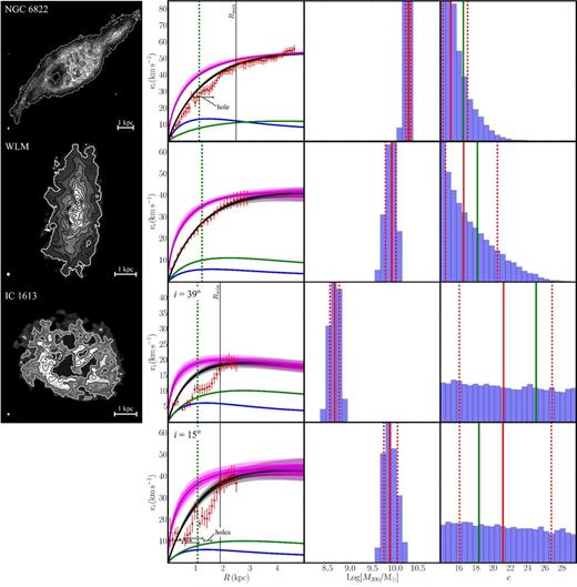
Rotation curve models for three isolated dwarf irregular galaxies: NGC 6822 (top); WLM (middle); and IC 1613 (bottom). For IC 1613, we show results for two different inclination angles: i = 39° and i = 15°, as marked. The columns show from left to right: the H i column density map with size-scale and beam-size marked; the rotation curve data; and histograms of M200 and c from our emcee model chains. For the latter three panels, the lines and symbols are as in Fig. 2. On the rotation curve plot (second column), we mark the position of H i holes seen in the column density map (leftmost column) of NGC 6822 and IC 1613. On the concentration parameter plot (rightmost column), we mark the cosmological mean cΛCDM (vertical green line), expected for a halo with the median M200 from our model chains.
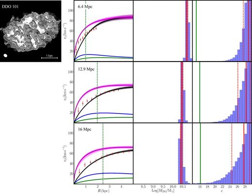
Rotation curve models for DDO 101. From top to bottom, the rows show results assuming three different distances to the dwarf D = 6.4 Mpc (as assumed previously in the literature); D = 12.9 Mpc (the Hubble flow distance); and D = 16 Mpc (the maximum distance reported in the literature). The columns lines and symbols are as in Fig. 5.
NGC 6822 and WLM
The top two rows of Fig. 5 show our results for NGC 6822 and WLM. The columns show, from left to right: the H i column density map with size-scale marked; the rotation curve data; and histograms of M200 and c from our emcee model chains. For the latter three panels, the lines and symbols are as in Fig. 2.
The rotation curve for NGC 6822 shows a clear dip just beyond the projected half stellar mass radius. This could owe to the prominent H i bubble that is present at this location, or to the possible presence of a stellar bar or misaligned stellar component (see discussion in Section 3 and Section 5.3); beyond ∼2.5 kpc the rotation curve and H i column density map are quite smooth. Since our simple rotation curve model is not able to capture such complexities, we exclude the inner region (<2.5 kpc) from our fits. None the less, our simple model with just three free parameters (M200; c and the disc stellar mass M*) gives a remarkable match to the data over the full rotation curve from 0 to 5 kpc. We obtain tight constraints on M200 and a concentration parameter in excellent agreement with cosmological expectations (see the vertical green line in the rightmost panel that marks cΛCDM derived from the median M200 using the relation in Macciò et al. 2007). The priors used for this fit and our derived values for M200 and c with 68 per cent confidence intervals are reported in Table 1. As in Fig. 2, the magenta lines overlaid on the rotation curve show what our model rotation curves look like if we switch off cusp-core transformations (i.e. if we input our fitted coreNFW parameters to the NFW profile and calculate the resulting rotation curves). Notice that the dark matter core in NGC 6822 affects the rotation curve out to ∼2R1/2 (vertical dashed green line), as expected from equation (22) and our discussion in Section 4.1.
Similarly to NGC 6822, our model gives an excellent match to WLM's rotation curve over its full range from 0 to 3 kpc. We obtain good constraints on M200 and – like NGC 6822 – a concentration c consistent with cosmological expectations. As with NGC 6822, it is important that we fit with our coreNFW profile rather than the NFW profile, since the latter leads to rotation curves that rise substantially more steeply than the data (compare the magenta and black lines in the rotation curve data panel).
Both NGC 6822 and WLM have rather low best-fitting |$\chi ^2_{\rm red}$| (see Table 1), with |$\chi ^2_{\rm red} = 0.36$| and |$\chi ^2_{\rm red} = 0.26$|, respectively. Such low values are typical of rotation curve fits and owe in part to the way in which the error bars and derived, and in part – for NGC 6822 – to the limited radial range over which the data are fit (see e.g. Sellwood & Sánchez 2010; Hague & Wilkinson 2013). Indeed, if we exclude the ‘dip’ region inside 0.5 kpc for our mock dwarf from Section 5.3 (Fig. 4, top middle panel), then we find a best-fitting |$\chi ^2_{\rm red} = 0.37$|, similar to that for NGC 6822.
IC 1613: a near face-on disequilibrium dwarf
In contrast to our excellent fits for WLM and NGC 6822, IC 1613 gives a very poor fit (compare the black lines with the red data points in the rotation curve panel). If fitting over the full data range, our model pushes on the lower bound of our M200 prior since it cannot reproduce the extremely shallow rise of IC 1613's rotation curve. For this reason we exclude the inner region, fitting over the range [1.9, 2.5] kpc. (This explains why the reduced |$\chi _{\rm red}^2 = 0.13$| reported in Table 1 seems surprisingly good despite the obviously poor fit.)
The poor fit for IC 1613 is perhaps not surprising when considering its gas morphology. IC 1613 shows substantial H i bubbles in its H i column density map (leftmost panel) that are qualitatively very similar to the starburst simulation in Fig. 2; it also presents substantially more recent star formation than all of the other dwarfs considered here, consistent with a starburst (see Section 3). Most notably, its rotation curve shows prominent wiggles and rises far less steeply than our model would predict given its projected half stellar mass radius.
The shallow rise of IC 1613's rotation curve is reminiscent of our mock starbursting dwarf inclined at itrue = 15° that we discussed in Section 5.3. There, we showed that for itrue ≲ 30°, 3DBarolo systematically overestimates the inclination leading to an artificially shallow rise in the rotation curve. The favoured inclination for IC 1613 from 3DBarolo is ifit = 39 ± 2° (see Table 1), similar to that derived by Little THINGS (Oh et al. 2015). However, our mock data analysis in Section 5.3 indicates that at this low inclination, the true inclination could be as low as itrue ∼ 15°. In the bottom row of Fig. 5, we consider what the rotation curve for IC 1613 would look like at such an inclination. Now, similarly to our near face-on mock dwarf, the rotation curve rises substantially more steeply. It is well fit by our coreNFW model except at ∼0.5 and ∼1.5 kpc, where there are prominent H i bubbles. This is similar to the inner region of NGC 6822, where its bubble also appears to cause a depression in the rotation curve, and to our mock rotation curve that we discussed in Section 5.3. The mass derived from the rotation curve for IC 1613 is now dramatically different, rising over a dex to |$M_{200} = 8_{-2}^{+4}\times 10^9$| M⊙ (see Table 1).
With an inclination of ifit < 40°, we conclude that it is challenging to recover the true inclination of IC 1613. This is further exacerbated by the fact that it is a starbursting dwarf with prominent fast moving H i bubbles (see Section 3). We will consider in future work whether improvements to 3DBarolo can yield a more trustworthy measure of its inclination. Until such time, galaxies like IC 1613 are not well-suited for testing ΛCDM.
DDO 101: the perils of distance uncertainty
Finally, we consider the interesting and substantially more distant dwarf irregular, DDO 101. The nearest dwarf irregulars to us (D ≲ 3 Mpc) have reliable distances as measured from either Cepheid variable stars or the ‘tip-of-the-red-giant’ branch method (e.g. McConnachie 2012). Very distant dwarfs with D ≳ 10 Mpc enter the Hubble flow and we can also obtain a reliable distance from their redshift alone (e.g. Peñarrubia et al. 2014). However, for dwarfs at intermediate distances 3 ≲ D ≲ 10 Mpc, like DDO 101, we are forced to rely on the ‘Tully–Fisher’ (TF) distance method (Tully & Fisher 1977). This uses the TF relation to obtain the absolute magnitude of the dwarf from its observed peak rotation velocity. Comparing this with the apparent magnitude then allows us to derive its distance. This is problematic for two reasons. First, there is enormous scatter in the TF relation, particularly at low peak rotation velocities (e.g. Meyer et al. 2016). Secondly, many dwarfs have rising rotation curves and thus their peak rotation velocity is only a lower bound on the true peak. These difficulties lead to distance errors that can be as large as a factor of 2 or more. Indeed, the quoted distance range for DDO 101 on the NED data base is 6.4 < DDDO101/Mpc < 16. Yet to date, it as been mass modelled assuming DDDO101 = 6.4 Mpc (Oh et al. 2015).
In Fig. 6, we show results from mass modelling DDO 101 assuming three different distances DDDO101 = 6.4 Mpc (as assumed previously in the literature; top row); DDDO101 = 12.9 Mpc (the Hubble flow distance, using the cosmological parameters from Planck Collaboration XVI 2014; middle row); and DDDO101 = 16 Mpc (the maximum distance reported in NED; bottom row). For DDDO101 = 6.4 Mpc, the fit is poor. The rotation curve rises much more steeply than is allowed by the coreNFW model, similarly to the findings in Oh et al. (2015). Indeed, the fact that DDO 101 is one of the few isolated dwarf irregulars with a rotation curve that appears ‘NFW-like’ was the key motivation for including it in our sample here. However, if we place DDO 101 at a larger distance – as preferred by its redshift – then the rotation curve is stretched and rises much less steeply. The middle and bottom rows of Fig. 6 show our results assuming DDDO101 = 12.9 Mpc and DDDO101 = 16 Mpc, respectively. In both cases, we obtain an excellent fit to the rotation curve, similarly to NGC 6822 and WLM. Note, however, that unlike those galaxies, DDO 101's rotation curve still rises sufficiently steeply that the favoured concentration parameter c pushes on the upper bound of our prior. We would need a higher resolution H i map of similar quality to WLM, and a more accurate measure of DDDO101, to determine whether or not this is something to worry about in the context of ΛCDM; for now, models with a cosmologically reasonable c are still allowed by the data.
The Baryonic Tully–Fisher Relation (BTFR)
The Baryonic Tully–Fisher Relation (BTFR) is a well-known correlation between the total baryonic mass of galaxies (stars plus gas; Mb) and their peak rotation velocity (Vf; e.g. McGaugh et al. 2000; McGaugh & Wolf 2010; McGaugh 2012; Lelli, McGaugh & Schombert 2016). In Fig. 7, we plot our four isolated dwarfs in the Vf − Mb plane (red/green data points) compared to a large sample of gas rich dwarfs taken from McGaugh (2012) (blue data points). Interestingly, our two ‘good’ galaxies – WLM and NGC 6822 lie within the 1σ scatter of the relation (green data points), whereas our two ‘problem galaxies’, IC 1613 and DDO 101 are both significant outliers (red data points). However, if we assume DDDO101 = 12.9 Mpc and iIC1613 ∼ 15° – as favoured by their coreNFW rotation curve fits – then both galaxies become consistent with the BTFR (green data points). This is encouraging as it implies that with our favoured distance and inclination for DDO 101 and IC 1613, respectively, these two dIrrs become very similar to other dIrrs of similar baryonic mass. This behaviour was noted also in Oman et al. (2016) where they pointed out that for IC 1613 a mean inclination of i ∼ 22° would be required to bring it on to the BTFR, similarly to what we find here.
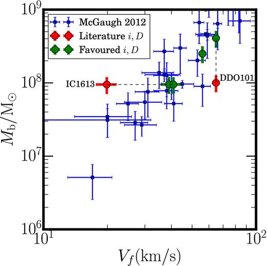
The four isolated dIrrs analysed in this paper (red/green data points) as compared to the BTFR of galaxies taken from McGaugh 2012 (blue data points). Notice that with the literature values, IC 1613 and DDO 101 are outliers from this relation (red data points), but with our favoured inclination and distance of iIC1613 ∼ 15° and DDDO101 = 12.9 Mpc, respectively, they become perfectly consistent (green data points).
CONCLUSIONS
In the first part of this paper, we used mock data from high resolution simulations of isolated dwarf galaxies to understand the shape and diversity of dwarf galaxy rotation curves in ΛCDM. Our key findings were as follows. We then went on to fit mass models, using a new coreNFW profile that accounts for cusp-core transformations due to stellar feedback, to real data for four isolated dwarf irregular galaxies. These were chosen to span an interesting range of rotation curve morphologies: NGC 6822; WLM; IC 1613; and DDO 101. Our key results were as follows.
The rotation curve in our mock dwarfs systematically shifts up and down in amplitude throughout the starburst cycle. At its most quiescent phase, the asymmetric drift corrected gas rotational velocities give a good match to the true circular speed curve. Following a strong starburst, however, the rotation curve rises more steeply, while just post-starburst it rises substantially less steeply. Such ‘disequilibrium’ galaxies can be readily identified, however, by the presence of substantial fast-moving H i bubbles (with expansion velocity ∼10–30 km s−1). Our simulated dwarfs continually cycle through quiescent, starburst and post-starburst phases suggesting that all three situations should be common. Indeed, many real starbursting dwarfs show kinematically disturbed H i discs (e.g. Lelli, Verheijen & Fraternali 2014).
Fitting a new coreNFW profile (that accounts for dark matter cusp-core transformations due to stellar feedback) to the above mock rotation curve data, we found that we could successfully recover the virial mass M200 and concentration parameter c of our mock data, but only if we fit the rotation curve in its quiescent phase. The starburst and post-starburst mocks led to a systematic under-estimate of M200 by up to half a dex, and a biased concentration parameter c.
It is important to use the coreNFW profile rather than an NFW profile in the mass models. The NFW profile rotation curves rise too steeply to be consistent with our mock data and lead to a substantial bias on M200 and/or c if used instead of the coreNFW profile.
We tested our recovery of the rotation curve from mock H i data cubes, using the 3DBarolo code. We found that we could obtain an excellent recovery of the rotation curve, provided its best-fitting inclination was ifit ≳ 40°. Lower inclinations than this are systematically biased high, leading to rotation curves that have an artificially shallow rise, with an associated underestimate of M200 of up to a dex or more.
The stellar kinematics are substantially less affected by the starburst cycle than the gas kinematics. This might suggest that for starburst or post-starburst systems, stars will be a more reliable probe of the underlying potential than the H i rotation curve. However, stars probe the potential only out to R1/2, making them a poor probe of the halo virial mass M200, as discussed in R16. Thus, even when including stellar kinematic data, it is probably best to avoid galaxies that show signs of having a gaseous rotation curve that is far from equilibrium.
We obtained excellent fits for NGC 6822 and WLM, with tight constraints on M200, and concentration parameters c consistent with cosmological expectations (see Table 1 and Fig. 5).
By contrast, both IC 1613 and DDO 101 gave a very poor fit. For IC 1613, we showed that this owes to substantial fast moving H i bubbles and a poorly determined inclination; for DDO 101, the problem was its uncertain distance. Using iIC1613 ∼ 15° and DDDO101 ∼ 12 Mpc, consistent with current uncertainties, we were able to fit both galaxies very well (see Table 1 and Figs 5 and 6). Interestingly, with this inclination and distance, IC 1613 and DDO 101 also become consistent with the ‘Baryonic Tully–Fisher Relation’ of galaxies (Fig. 7).
Although in this paper we have only analysed a small sample of four dwarf irregular galaxies, we have deliberately picked some of the most challenging rotation curves for ΛCDM reported in the literature to date. It is encouraging, then, that all four are well-fit by our coreNFW model once errors in the inclination and distance are properly taken into account. This suggests that the now long-standing ‘cusp-core’ problem owes to previously unmodelled ‘baryonic’ physics (bursty star formation driven by stellar feedback), while the newer ‘dwarf rotation curve diversity’ problem likely owes to a mixture of inclination and distance error, and disequilibria driven by fast moving H i bubbles. There are, however, other sources of rotation curve scatter that we have not considered here, including cosmological scatter on the coreNFW model parameters that we only briefly explored in Appendix C, and the effect of galaxy mergers and interactions. We will consider the effect of these, and confront our coreNFW model with a larger sample of dwarf irregulars in forthcoming papers.
JIR and OA would like to acknowledge support from STFC consolidated grant ST/M000990/1. JIR acknowledges support from the MERAC foundation. OA would like to acknowledge support from the Swedish Research Council (grant 2014-5791). This research made use of aplpy, an open-source plotting package for python hosted at http://aplpy.github.com; PyNbody for the simulation analysis (https://github.com/pynbody/pynbody; Pontzen et al. 2013); and the emcee package for model fitting (http://dan.iel.fm/emcee/current/). All simulations were run on the Surrey Galaxy Factory. The research has made use of the NASA/IPAC Extragalactic Database (NED) which is operated by the Jet Propulsion Laboratory, California Institute of Technology, under contract with the National Aeronautics and Space Administration. We would like to thank Se-Heon Oh and Little THINGS for kindly making their data public; and Erwin de Blok for kindly providing the data for NGC 6822. We would like to thank Jorge Peñarrubia; Octavio Valenzuela; Malcolm Fairbairn; Chris Brook; Benoit Famaey and the anonymous referee for useful comments that improved this manuscript.
The simulations in R16 do miss some potentially important physics, for example magnetic fields, radiative transfer, dust and cosmic rays. However, the excellent agreement with a wide range of data for isolated dwarf irregulars, without any fine-tuning of the simulation parameters, suggests that these missing physics are next-to-leading order effects. For further discussion of these points, see R16.
More precisely, the total duration of star formation, not to be confused with the star formation depletion time-scale tdep = Σgas/ΣSFR (e.g. Bigiel et al. 2011).
Note that the true ‘size’ of the dark matter core is somewhat arbitrary and depends on what definition we use (see e.g. the discussion in Goerdt et al. 2006). From R16, their fig. 4, the onset of the dark matter core occurs visually at ∼R1/2 and hence we refer throughout this paper to the dark matter core being of ‘size’ ∼R1/2. To reproduce this behaviour with the coreNFW model, however, we require that our ‘core size’ parameter rc is nearly twice R1/2, as in equation (21).
Since the stars and gas are sub-dominant to the dark matter at all radii, for this ‘true rotation curve’, we assume spherical symmetry such that |$v_c^2 = GM_{\rm tot} / R$|, where Mtot is the total enclosed mass, as calculated from the gravitational potential.
REFERENCES
APPENDIX A: THE EFFECT OF VARYING THE ASYMMETRIC DRIFT CORRECTION
In this appendix, we explore the effect of six different asymmetric drift (AD) corrections on the derived rotation curve for WLM. In each case, we solve equation (10) assuming different radially varying gas surface density profiles Σgas(R) and assuming either a fixed gas velocity dispersion, or one that is also radially varying (as measured from the data).
EF: this is an exponential, constant velocity dispersion, AD correction described already in Section 2.1.1.
E: the is an exponential AD correction, but using the measured radially varying velocity dispersion.
- CEF: this is a core+exponential AD correction that assumes the following functional form:where I0, R0 and α are fitting parameters, and we assume a fixed velocity dispersion σgas = const.(A1)\begin{equation} \Sigma _{\rm gas} \sigma _{\rm gas}^2 = \frac{I_0 (R_0 + 1)}{R_0 + e^{\alpha R}} \end{equation}
CE: this is a core+exponential AD correction with radially varying velocity dispersion.
- HEF: this is a hole+exponential AD correction:with fixed velocity dispersion.(A2)\begin{equation} \Sigma _{\rm gas} \sigma _{\rm gas}^2 = I_0 \left(1 + \frac{R}{R_0}\right)^{\alpha } e^{-\frac{R}{R_0}} \end{equation}
HEF: this is a hole+exponential AD correction with radially varying velocity dispersion.
The derived rotation curve for WLM in each case agrees within our 1σ uncertainties. In Fig. A1, we show the M200 and c derived from these rotation curves, with 68 per cent confidence intervals marked for each case (each data point is labelled with its correction). Notice that the error bars for both M200 and c overlap in all cases. There is a systematic trend for the exponential correction to systematically favour lower M200 and higher c, but it is not statistically significant. For the mock data, we use the EF correction since an exponential gives a good fit to the gas surface density profile while the velocity dispersion profile is found to be very close to constant; for the real data we favour the CE correction since this gives a slightly better representation of the H i data. The effect of these choices, however, is very small.
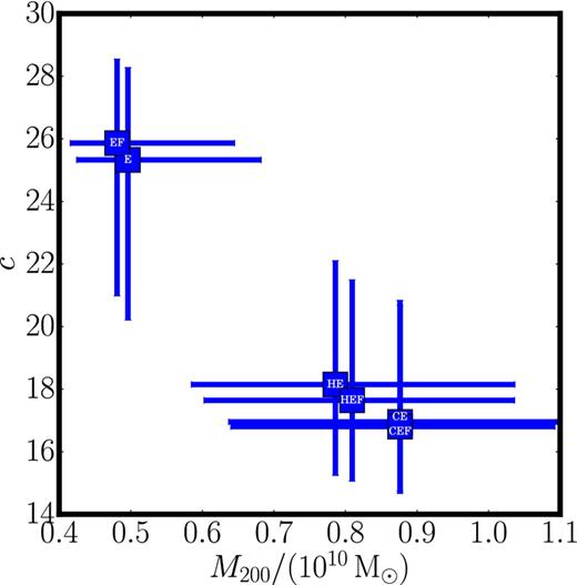
The effect of six different asymmetric drift corrections on the derived M200 and c for WLM. The corrections are described in Appendix A and marked at the centre of each data point. Notice that in all cases, the derived M200 and c overlap within our quoted uncertainties.
APPENDIX B: FITTING NFW INSTEAD OF coreNFW
In this appendix, we explore the effect of fitting an NFW profile to our mock data instead of our coreNFW profile (see Section 4 for a description of both profiles). In Fig. B1, we show fits to our mock rotation curve for our quiescent M200 = 109 M⊙ dwarf, but assuming an NFW profile for the dark matter halo. The top row shows a fit using all of the data to R = 1.5 kpc. Since this reaches out to where the rotation curve is flat, we still recover the correct M200. The concentration parameter is, however, biased towards low c and pushes on our theory prior. The bottom row shows the same fit but excluding data for R > 1 kpc. Now, in order to fit the shallow rise of the rotation curve, the NFW profile is pushed towards systematically low M200.
The effect of fitting the NFW profile instead of coreNFW to our mock data. The lines and symbols are as in Fig. 2. The top row shows a fit to the mock rotation curve for our quiescent M200 = 109 M⊙ dwarf. Since the data reach to R = 1.5 kpc where the rotation curve is flat, we still recover the correct M200. The concentration parameter is, however, biased towards low c and pushes on our prior. The bottom row shows the same fit but excluding data for R > 1 kpc. Now in order to fit the shallow rise of the rotation curve, the NFW profile is pushed towards systematically low M200.
APPENDIX C: ALLOWING THE DARK MATTER CORE SIZE TO VARY
By default, we have assumed throughout this paper that the dark matter core size parameter η = 1.75 (equation 21) is held fixed. This gave the best match to our simulations in R16. However, as discussed in R16, there could be some scatter on η due to varying halo spin, concentration parameter and/or halo assembly history. For this reason, in this appendix we explore allowing η to vary freely over the range 0 < η < 5 when fitting data for WLM. The results are shown in Fig. C1. As might be expected, allowing η to vary limits our ability to measure the halo concentration parameter c and slightly inflates our errors on M200. Otherwise, however, its effect is benign. Interestingly, we find |$\eta _{\rm WLM} = 2.4_{-0.52}^{+0.78}$| at 68 per cent confidence, consistent with our favoured η = 1.75 and clearly inconsistent with a dark matter cusp (η = 0).
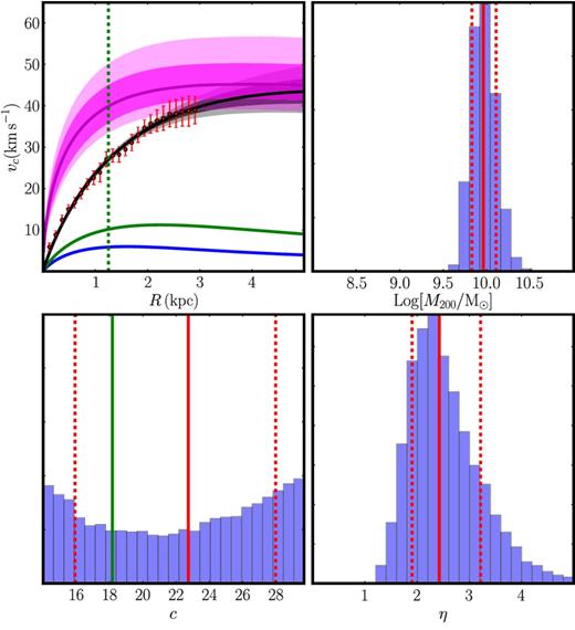
The effect of allowing the dark matter core size to freely vary when fitting data for WLM. The lines and symbols are as in Fig. 2. Recall that the dark matter core size is set by equation (21): rc = ηR1/2 and is therefore controlled by the dimensionless parameter η. In this fit to WLM's rotation curve, we allow 0 < η < 5; the histogram of recovered η from our model chains is shown in the bottom right panel. Notice that the data clearly favour a dark matter core over a cusp (η = 0), while our favoured value of η = 1.75 from R16 is recovered at the edge of our 68 per cent confidence intervals.
APPENDIX D: THE EFFECT OF THE CONCENTRATION PARAMETER PRIOR
Fig. D1 shows the density of our MCMC models (ρmodels) projected on to the c − M200 plane for WLM. The red contours show the results for our most generous logarithmic prior that allows c to extend to cosmologically inconsistent values; the black contours show the same for our already generous default prior; and the blue contours show results for a very restrictive ‘cosmology’ prior that demands that c exactly obeys the concentration–mass relation in equation (D1). In all cases, the contours mark 10 logarithmically spaced isodensity contours of the MCMC models over the range 0.01 < ρmodels < 1, where ρmodels is normalized such that max (ρmodels) = 1. As can be seen, for the default and logarithmic prior there is a ‘banana’ degeneracy between M200 and c, while models with low c are weakly favoured. This trend to low c is, however, not statistically significant. The best |$\chi ^2_{\rm red}$| for the restrictive cosmology prior was |$\chi ^2_{\rm red} = 0.1$| as compared to |$\chi ^2_{\rm red} = 0.08$| for the logarithmic prior. Rather, this behaviour simply indicates that the data are not able to give tight constraints on c and thus the marginalised distribution of c depends wholly on our priors.

The effect of varying the prior on the concentration parameter c for WLM. The red contours show the density of our MCMC models (ρmodels) in the c − M200 plane for our most generous logarithmic prior (that allows c to extend to cosmologically inconsistent values); the black contours show the same for our already generous default prior; and the blue contours show results for a very restrictive ‘cosmology’ prior that demands that c exactly obeys the concentration–mass relation in equation (D1). In all cases, the contours mark 10 logarithmically spaced isodensity contours of the MCMC models over the range 0.01 < ρmodels < 1, where ρmodels is normalized such that max (ρmodels) = 1.
Finally, we may reasonably ask if the higher M200 allowed by the logarithmic prior are acceptable models for WLM. In the sense that they fit the rotation curve data, they are acceptable models. However, such haloes lie far from the cosmic mean concentration parameter and so are not expected in ΛCDM. (From equation D1, we expect a halo of mass log10M200 = 10.5 to have c10.5 ∼ 16.) Thus, our default prior on c is a compromise between allowing c to vary over a generous range while disallowing haloes that are unlikely to exist in ΛCDM.
