


Abstract
Modelling of massive stars and supernovae (SNe) plays a crucial role in understanding galaxies. From this modelling we can derive fundamental constraints on stellar evolution, mass-loss processes, mixing, and the products of nucleosynthesis. Proper account must be taken of all important processes that populate and depopulate the levels (collisional excitation, de-excitation, ionization, recombination, photoionization, bound–bound processes). For the analysis of Type Ia SNe and core collapse SNe (Types Ib, Ic and II) Fe group elements are particularly important. Unfortunately little data is currently available and most noticeably absent are the photoionization cross-sections for the Fe-peaks which have high abundances in SNe. Important interactions for both photoionization and electron-impact excitation are calculated using the relativistic Dirac atomic R-matrix codes (darc) for low-ionization stages of Cobalt. All results are calculated up to photon energies of 45 eV and electron energies up to 20 eV. The wavefunction representation of Co iii has been generated using grasp0 by including the dominant 3d7, 3d6[4s, 4p], 3p43d9 and 3p63d9 configurations, resulting in 292 fine structure levels. Electron-impact collision strengths and Maxwellian averaged effective collision strengths across a wide range of astrophysically relevant temperatures are computed for Co iii. In addition, statistically weighted level-resolved ground and metastable photoionization cross-sections are presented for Co ii and compared directly with existing work.
1 INTRODUCTION
Lowly ionized species of Cobalt are often observed in astrophysical objects such as supernovae (SNe), cool stars (Bergemann, Pickering & Gehren 2010), early-type stars (Smith & Dworetsky 1993) and the solar spectrum (Pickering et al. 1998). These applications necessitate the need for high-quality atomic data which accurately describe the processes of excitation and photoionization. This is further evidenced in SNe by following the nucleosynthesis decay path of 56Ni→ 56Co→ 56Fe, which occurs post explosion. Our principal aim is to facilitate modelling within the astrophysics community with accurate and up-to-date atomic transitions necessary for synthetic spectral analysis, allowing detailed comparisons to be carried out with observation. Stand-alone reports stress both the importance and absence of photon/electron interaction with systems of Iron, Cobalt and Nickel (Ruiz-Lapuente 1995; Hillier 2011; Dessart et al. 2014).
The photoionization cross-sections are to be implemented into the 3D plus time-dependent computer code artis, which models the ejecta of Type Ia SNe as discussed in detail by Sim (2007); Kromer & Sim (2009). Currently, only hydrogenic approximations, or fits to the cross-sections are incorporated into the codes. It is our aim to provide ground and excited state contributions to all possible final states. The code is based on a similar approach by Lucy (2005), where methods for treatment of the transporting radiation, kinetic energies, and ionization energies are considered to compute light curves for particular models and symmetries.
The Opacity Project has been an invaluable source for such data, but is often limited when considering Fe-peak species (Cunto & Mendoza 1992; Cunto et al. 1993). These important Fe-peaks are difficult to investigate due to their open d-shell structure which gives rise to many hundreds of target states for each electronic configuration and typically thousands of closely coupled channels. Hence the target states require substantial configuration interaction expansions for their accurate representation. Fe ii is one such challenging case where over the last decade calculations for this ion have grown in size, complexity and sophistication. Significant differences, however, are still observed in the resulting atomic data as can be seen by the latest two major evaluations for the electron-impact excitation of Fe ii (Ramsbottom et al. 2007; Bautista et al. 2015). Factors of 2 to 3 disparity being the norm at the temperature of maximum abundance 104 K for many of the low-lying forbidden lines.
There have been a number of studies focused on essential atomic data between species of Co i-iii concerning bound transitions. These include oscillator strengths for neutral Cobalt between 2276 and 9357 Å (Cardon et al. 1982), transition probabilities through a multiconfiguration approach for comparison with observed infrared spectra (Nussbaumer & Storey 1988), and also a relativistic Hartree–Fock approach between the lowest 47 levels of Co ii (Quinet 1998). More recently, collision strengths and other radiative data have been calculated for Co ii (Storey, Zeippen & Sochi 2016) and Co iv (Aggarwal et al. 2016). During the preparation of this work, it has come to our attention a detailed study of electron-impact excitation cross-sections for Co iii conducted by Storey & Sochi (2016), which we shall compare with in Sections 2 and 3.
The early ion stages of, and even neutral Cobalt are clearly important as detailed in the literature. Early observations has shown strong Co ii lines in η Carinae (Thackeray 1976), confirmed more recently by Zethson et al. (2001) to be unusually strong, and in the UV regime in ζ Oph (Snow, Weiler & Oegerle 1979), confirmed by Federman et al. (1993). These lines are apparent in the binary star HR5049 (Dworetsky, Trueman & Stickland 1980; Dworetsky 1982) – which previously have been unidentified due to the lack of laboratory data. In this same study, the amount of Cobalt is estimated to be around 3.0 dex overabundant relative to the Sun.
Due to the decay path of 56Ni, Cobalt is often observed in various SNe at both early and late epochs. The Type II SNe 1987A, exploded in the large magellanic cloud, providing a study of the expanding ejecta as the 56Co decays. A large proportion of Fe ii and Co ii lines are blended due to their similar ionization energies, but the strong 1.547 μm line occurs from the transition a5F5 → b3F4 (Meikle et al. 1989; Li, McCray & Sunyaev 1993) in Co ii. The Co iii a4F9/2 → a2G9/2 0.589 μm line in another Type II SNe, 1991bg, is used as a diagnostic to infer the mass of synthesized 56Ni. It is also possible to deduce important properties such as the mass of the exploding star (Mazzali et al. 1997).
The Co ii and Co iii ions under discussion in this publication have also received much interest over the last decade. The mid-infrared spectrum of SNe 2003hv and 2005df show strong Co iii line emissions and even emission from Co iv (Gerardy et al. 2007). However, the collisional processes included in the model have been approximated using statistically weighted collision strengths. A study of the near-infrared spectra from SNe 2005df yields strong Co iii emission lines initially but by day 200 the majority of Cobalt has expectedly decayed down to Fe (Diamond, Hoeflich & Gerardy 2015). A number of Co iii lines are still visible at late times for Type Ia SNe as documented in (Ruiz-Lapuente 1995). These lines would be extremely beneficial in particular diagnostic work, but as outlined above, little collisional data exists. In addition the photoionization cross-sections employed in the models are obtained from a central potential approximation (Reilman & Manson 1979) for the ground state only. Co iii is also present in SNe 2014J and the 11.888 μm line is useful for monitoring the time evolution of the photosphere, and again, the mass of synthesized Ni (Telesco et al. 2015). It is evident from these works and the associated applications the importance of conducting sophisticated and complete calculations for the lowly ionized Fe-peak species of Fe, Ni and Co.
In Section 2, we discuss the development of an accurate structure model for Co iii to include in the R-matrix collisional calculations for electron-impact excitation and photoionization. The accuracy of this model will be tested by reassessing energy levels of the target states and the conformity of transition probabilities with previous assessments. In Section 3, we present level-resolved ground and excited state photoionization cross-sections for Co ii and a selection of collision strengths and effective collision strengths for the electron-impact excitation of Co iii. Comparisons will be made where possible with existing data but these are limited. Finally we summarize our findings and conclusions in Section 4.
2 IMPORTANT TRANSITIONS FOR SYNTHETIC SPECTRAL MODELLING
This paper focuses initially on transitions that occur between discrete states of our atomic system, Co iii. In Fig. 1, we graphically present some of the most important lines in the infrared and visible energy bands of the spectrum. Transitions among the ground state term 4F and levels of the parent ion Co iii with configuration 3d7 are shown on the right-hand side. The neighbouring system Co ii is also shown on the left complete with its fine-structure split J levels to indicate the photoionization process under investigation.
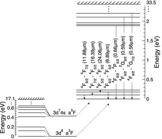
Important lines in the infrared and visible energy bands between levels of Co iii amongst the 3d7 configuration and involving the ground term 4F. The neighbouring system of Co ii is to the left with its split J levels to indicate the photoionization process.
2.1 Target description and bound state transitions
As stated in the introduction, partially filled d-shell systems are difficult due to the hundreds of levels associated with a single configuration. Initially, we include three configurations, 3d7 and 3d6[4s, 4p] during the optimization process, denoted as model 1, which results in a total of 262 fine structure levels to describe the Co iii ion. The ground state of which is 3d7a4F9/2. Next we optimize all orbitals up to 3d on the configurations from the double electron promotions, 3s2, 3p2 → 3d2 and include in the total calculation all configurations from model 1 plus 3p63d9 (double promotion from 3s to 3d) and 3s23p43d9 (double promotion from 3p to 3d). This technique can be useful as it alleviates the necessity to include numerous pseudo-states into the calculation. We denote this model 2 which constitutes a total of 292 levels. Finally, by including 3d5[4s2, 4p2] and 3d54s4p, the number of levels drastically increases to 1259 levels, and we label this as model 3.
We present in Table 1 our ab initio energy levels obtained from grasp0 in eV for the lowest lying 50 levels alongside those observed by Sugar & Corliss (1985). We also present the per cent difference between Sugar & Corliss (1985) and our model 2, and also provide the lowest 15 levels of Storey & Sochi (2016). Good agreement is found (<10 per cent for the majority of levels) between the present model 2 and model 3 energies and those of Storey & Sochi (2016). As with other Fe-peak ions, the energy levels of the lowest-lying 3d7 fine-structure states are notoriously difficult to determine. The highest disparities are found for these levels when compared with Sugar & Corliss (1985), the largest being for the 3d74F9/2 → 3d72H11/2 (1-12) transition. For levels indexed above 17 the differences are at most 10 to 11 per cent and for many levels by considerably less. The main problem is due to the fact that a single 3d orbital is used to describe the configuration state functions for multiple configurations of type 3d7 and 3d64s. Similar differences were reported by Ramsbottom (2009) for the low-lying 3d7 fine-structure levels of Fe ii. Despite the high per cent differences found between these lowest levels in Table 1, overall the average per cent change across the 171 Sugar & Corliss (1985) Jπ symmetries is a more acceptable 6.2 per cent. The differences between model 2 and model 3 are not significant enough to justify the much larger calculation, and we can also benefit by employing all 292 levels into the close-coupling wavefunction expansion of the Co iii. We therefore adopt our model 2 as the final model for the scattering calculation.
Energies for the lowest 50 levels of Co iii are presented in eV relative to the ground state 3d7 a4F9/2. S&C is from the work of Sugar & Corliss (1985). model 1, model 2, model 3 are the current results from grasp0 and the last column are the lowest 15 levels from Storey & Sochi (2016). We also present the per cent difference between our current model 2 and S&C in the 6th column.
| Index | Level | S&C | Model 1 | Model 2 | Per cent | Model 3 | Storey |
|---|---|---|---|---|---|---|---|
| 1 | 3d7 a4F9/2 | 0.000 00 | 0.000 00 | 0.000 00 | 0.0 | 0.000 00 | 0.000 00 |
| 2 | 3d7 a4F7/2 | 0.104 30 | 0.103 55 | 0.099 39 | 4.7 | 0.099 80 | 0.102 16 |
| 3 | 3d7 a4F5/2 | 0.179 94 | 0.180 01 | 0.172 55 | 4.1 | 0.173 21 | 0.177 05 |
| 4 | 3d7 a4F3/2 | 0.231 45 | 0.232 63 | 0.222 80 | 3.7 | 0.223 62 | 0.228 38 |
| 5 | 3d7 a4P5/2 | 1.884 80 | 2.394 05 | 2.204 36 | 16.9 | 2.197 61 | 2.293 69 |
| 6 | 3d7 a4P3/2 | 1.912 85 | 2.426 37 | 2.232 71 | 16.7 | 2.226 08 | 2.329 04 |
| 7 | 3d7 a4P1/2 | 1.960 36 | 2.472 83 | 2.278 75 | 16.2 | 2.272 44 | 2.370 33 |
| 8 | 3d7 a2G9/2 | 2.104 96 | 2.390 59 | 2.389 92 | 13.5 | 2.388 42 | 2.427 73 |
| 9 | 3d7 a2G7/2 | 2.202 73 | 2.489 67 | 2.482 50 | 12.7 | 2.481 38 | 2.523 95 |
| 10 | 3d7 a2P3/2 | 2.503 85 | 3.162 29 | 2.852 43 | 13.9 | 2.843 34 | 3.178 09 |
| 11 | 3d7 a2P1/2 | 2.593 56 | 3.270 65 | 2.964 28 | 14.3 | 2.956 73 | 3.282 36 |
| 12 | 3d7 a2H11/2 | 2.816 96 | 3.183 56 | 3.352 70 | 19.0 | 3.352 60 | 3.184 78 |
| 13 | 3d7 a2H9/2 | 2.905 48 | 3.268 36 | 3.431 16 | 18.1 | 3.431 43 | 3.270 58 |
| 14 | 3d7 a|$^2_2$|D5/2 | 2.858 93 | 3.446 72 | 3.062 77 | 7.1 | 3.047 40 | 3.447 26 |
| 15 | 3d7 a|$^2_2$|D3/2 | 3.004 98 | 3.603 58 | 3.231 40 | 7.5 | 3.218 73 | 3.599 63 |
| 16 | 3d7 a2F5/2 | 4.590 02 | 5.513 92 | 5.366 09 | 16.9 | 5.357 16 | – |
| 17 | 3d7 a2F7/2 | 4.626 66 | 5.558 37 | 5.408 63 | 16.9 | 5.399 98 | – |
| 18 | 3d64s a6D9/2 | 5.757 62 | 6.708 46 | 6.068 49 | 5.4 | 6.201 78 | – |
| 19 | 3d64s a6D7/2 | 5.827 64 | 6.789 42 | 6.146 50 | 5.5 | 6.279 25 | – |
| 20 | 3d64s a6D5/2 | 5.878 76 | 6.848 69 | 6.203 78 | 5.5 | 6.336 14 | – |
| 21 | 3d64s a6D3/2 | 5.913 87 | 6.889 47 | 6.243 24 | 5.5 | 6.375 36 | – |
| 22 | 3d64s a6D1/2 | 5.934 48 | 6.913 40 | 6.266 43 | 5.6 | 6.398 40 | – |
| 23 | 3d64s a4D7/2 | 6.909 54 | 8.420 15 | 7.722 55 | 11.8 | 8.049 98 | – |
| 24 | 3d64s a4D5/2 | 6.989 46 | 8.512 85 | 7.811 96 | 11.8 | 8.138 68 | – |
| 25 | 3d64s a4D3/2 | 7.041 66 | 8.573 68 | 7.870 84 | 11.8 | 8.197 22 | – |
| 26 | 3d64s a4D1/2 | 7.071 67 | 8.608 77 | 7.904 80 | 11.8 | 8.230 95 | – |
| 27 | 3d7 a|$^2_1$|D3/2 | – | 8.671 61 | 7.930 64 | – | 7.965 45 | – |
| 28 | 3d7 a|$^2_1$|D5/2 | – | 8.610 18 | 8.001 19 | – | 7.893 75 | – |
| 29 | 3d64s b4P5/2 | 8.794 71 | 10.250 65 | 9.638 34 | 9.6 | 9.809 74 | – |
| 30 | 3d64s a4H13/2 | 8.880 14 | 10.001 20 | 9.382 43 | 5.6 | 9.553 49 | – |
| 31 | 3d64s a4H11/2 | 8.911 21 | 10.031 98 | 9.412 43 | 5.6 | 9.583 37 | – |
| 32 | 3d64s a4H9/2 | 8.937 19 | 10.058 05 | 9.437 86 | 5.6 | 9.608 83 | – |
| 33 | 3d64s a4H7/2 | 8.960 40 | 10.080 57 | 9.459 63 | 5.6 | 9.630 75 | – |
| 34 | 3d64s b4P3/2 | 8.969 26 | 10.465 63 | 9.845 80 | 9.8 | 10.017 10 | – |
| 35 | 3d64s b4P1/2 | 9.077 44 | 10.594 39 | 9.970 61 | 9.8 | 10.140 09 | – |
| 36 | 3d64s b4F9/2 | 9.086 31 | 10.423 02 | 9.810 43 | 8.0 | 9.981 84 | – |
| 37 | 3d64s b4F7/2 | 9.117 82 | 10.460 16 | 9.846 05 | 8.0 | 10.016 92 | – |
| 38 | 3d64s b4F5/2 | 9.140 93 | 10.491 01 | 9.875 66 | 8.0 | 10.046 24 | – |
| 39 | 3d64s b4F3/2 | 9.157 70 | 10.515 40 | 9.898 93 | 8.1 | 10.069 29 | – |
| 40 | 3d64s a4G11/2 | 9.487 14 | 10.772 37 | 10.159 94 | 7.1 | 10.335 33 | – |
| 41 | 3d64s b2P3/2 | 9.520 88 | 11.328 10 | 10.679 64 | 12.2 | 10.964 74 | – |
| 42 | 3d64s a4G9/2 | 9.561 80 | 10.852 46 | 10.237 81 | 7.1 | 10.408 98 | – |
| 43 | 3d64s a4G7/2 | 9.594 28 | 10.886 42 | 10.271 10 | 7.0 | 10.441 58 | – |
| 44 | 3d64s b2H11/2 | 9.597 82 | 11.049 02 | 10.397 01 | 8.3 | 10.678 36 | – |
| 45 | 3d64s a4G5/2 | 9.605 34 | 10.895 26 | 10.280 19 | 7.0 | 10.451 25 | – |
| 46 | 3d64s b2P1/2 | 9.724 61 | 11.570 42 | 10.915 82 | 12.2 | 11.197 12 | – |
| 47 | 3d64s b2H9/2 | 9.624 02 | 11.082 83 | 10.429 07 | 8.4 | 10.713 76 | – |
| 48 | 3d64s b2F7/2 | 9.785 80 | 11.447 78 | 10.802 18 | 10.4 | 11.085 48 | – |
| 49 | 3d64s b2F5/2 | 9.847 49 | 11.533 72 | 10.882 86 | 10.5 | 11.168 01 | – |
| 50 | 3d64s b2G9/2 | 10.211 75 | 11.831 44 | 11.184 70 | 9.6 | 11.470 76 | – |

| i − j | Fivet | Hansen | Model 2 | Storey |
|---|---|---|---|---|
| 1 – 2 | 2.00 × 10⁻² | 2.00 × 10⁻² | 2.00 × 10⁻² | 2.00 × 10⁻² |
| 1 – 3 | – | 1.80 × 10⁻⁹ | 1.75 × 10⁻⁹ | – |
| 1 – 5 | 6.65 × 10⁻² | 4.80 × 10⁻² | 4.53 × 10⁻² | 5.55 × 10⁻² |
| 2 – 3 | 1.31 × 10⁻² | 1.30 × 10⁻² | 1.31 × 10⁻² | 1.31 × 10⁻² |
| 2 – 4 | – | 5.90 × 10⁻¹⁰ | 5.70 × 10⁻¹⁰ | – |
| 2 – 5 | 1.78 × 10⁻² | 1.35 × 10⁻² | 1.26 × 10⁻² | 1.51 × 10⁻² |
| 2 – 6 | 3.73 × 10⁻² | 2.70 × 10⁻² | 2.58 × 10⁻² | 3.14 × 10⁻² |
| 3 – 4 | 4.63 × 10⁻³ | 4.70 × 10⁻³ | 4.63 × 10⁻³ | 4.63 × 10⁻³ |
| 3 – 5 | – | 2.60 × 10⁻³ | 2.45 × 10⁻³ | 3.14 × 10⁻³ |
| 3 – 6 | 2.21 × 10⁻² | 1.63 × 10⁻² | 1.50 × 10⁻² | 1.85 × 10⁻² |
| 3 – 7 | 2.73 × 10⁻² | 2.00 × 10⁻² | 1.89 × 10⁻² | 2.30 × 10⁻² |
| 4 – 5 | – | 4.00 × 10⁻⁴ | 3.55 × 10⁻⁴ | – |
| 4 – 6 | – | 4.40 × 10⁻³ | 4.22 × 10⁻³ | 5.14 × 10⁻³ |
| 4 – 7 | 3.60 × 10⁻² | 2.60 × 10⁻² | 2.47 × 10⁻² | 3.02 × 10⁻² |
| 5 – 6 | – | 2.70 × 10⁻⁴ | 2.69 × 10⁻⁴ | – |
| 5 – 7 | – | 5.50 × 10⁻⁹ | 5.20 × 10⁻⁹ | – |
| 6 – 7 | – | 2.50 × 10⁻³ | 2.47 × 10⁻³ | 2.45 × 10⁻³ |
A much larger calculation for doubly ionized Fe-peak species has been performed recently by Fivet et al. (2016) using the same suite of codes as Hansen et al. (1984), and also by considering the computer package autostructure, (Eissner, Jones & Nussbaumer 1974; Badnell 1986), where the optimization process is carried out with a Thomas–Fermi–Dirac potential using lambda scaling parameters. Numerous doubly ionized ions of Fe, Ni and Co were considered in this publication. Single and double electron promotions out of the 3d, and also single electron promotions out of the 3s to the 5s orbital were included and comprised the basis expansion for both calculations. This is the most sophisticated and complete report for radiative rates in Co iii to date. Within the 3d7 complex, we vary approximately 27 per cent on average compared with both methods of Fivet et al. (2016).
2.2 The R-matrix method
To extend this problem to include interactions with photons and electrons, we consider the R-matrix method. A general overview of the theory can be found in Burke (2011). The theory was developed to perform electron scattering by Burke, Hibbert & Robb (1971) and extended for photoionization by Burke & Taylor (1975).
These calculations can be performed using a non-orthogonal B-spline basis set approach (Zatsarinny & Froese Fischer 2000; Zatsarinny & Bartschat 2004), intermediate-coupling frame transformation methods (Griffin, Badnell & Pindzola 1998) and one-body perturbation corrections to the non-relativistic Hamiltonian via the Breit–Pauli operators (Scott & Burke 1980) to name a few. In this paper, we consider the Dirac atomic R-matrix codes (darc) which includes relativistic effects through the Dirac Hamiltonian in equation (1) for this mid to heavy species ion. The wavefunctions obtained from grasp0 are formatted suitable for inclusion into darc. Validity of these methods between the outlined theoretical approaches are always important, and enhance the robustness of the techniques carried out as seen in Tyndall et al. (2016) for Ar+ and Fernández-Menchero, Del Zanna & Badnell (2015) for Al9 +. Therefore, it is possible to benchmark sophisticated experimental techniques against theory (Müller et al. 2009; Gharaibeh et al. 2011).
2.3 Photoionization
for initial and final scattering wavefunctions subject to the total dipole contribution. ω = hν is the photon energy or ω → ω−1 when considering the velocity operator, D. α is the fine structure constant, a0 is the Bohr radius and gi is the statistical weight of the initial state wavefunction. The summation is then carried out over all dipole-allowed transitions. The total wavefunctions Ψ are obtained from the momenta couplings with those wavefunctions obtained in Section 2.1. We represent these σp in units of Mb (≡ 10−18cm2) throughout this work.
The transitions of interest are calculated within the lowest eight fine-structure levels of Co ii pertaining to the two LSπ states as noted in equation (3). We also maintain a closed 3p6 core and are only concerned with low-energy transitions above threshold. Therefore, all even and odd allowed dipole symmetries up to J = 6 are calculated subject to the selection rules.
2.4 Electron-impact excitation
We calculate the main contribution to the collision strength defined in equation (4) from the partial waves up to J = 13 of both even and odd parity. These are obtained by considering appropriate total multiplicity and orbital angular momentum partial waves. However, in order to converge transitions at higher energies, we explicitly calculate partial waves up to J = 38 and use top-up procedures outlined in Burgess (1974) to account for further contribution to the total cross-section. The collision strengths can be extended to high-energy limits through an interpolation technique described by Burgess & Tully (1992).
3 RESULTS
As mentioned previously, the photoionization of Co ii and electron-impact excitation of Co iii rely on an accurate description of the Co iii wavefunctions. We are able to retain consistency throughout the calculation, and the fundamental R-matrix conditions apply to both processes. We select a total of 14 continuum basis orbitals per angular momenta to describe the scattered electron. The R-matrix boundary is then set at 10.88 au in order to enclose the radial extent of the 4p orbital. To make comparisons between observation, the target thresholds obtained in Table 1 have been shifted to those of Sugar & Corliss (1985).
3.1 Photoionization
In this section, we detail our results from the photoionization process described by equation (3). There is minimal atomic data for this interaction in the literature as only the total ground state transition exists. The first compilation is from Reilman & Manson (1979), using Hartree–Slater wavefunctions from a central field potential. Secondly, and more recently, Verner et al. (1993) have calculated cross-sections using the Hartree–Dirac–Slater potential and then applying an analytic fitting procedure. Recently, the Los Alamos suite of codes by Fontes et al. (2015) have been used to obtain results by a distorted wave method. For this we look at the photoionization of a 3d electron into the configuration averaged final states. To carefully resolve these spectra, we have employed a total of 200 000 equally spaced energy points over a photoelectron energy range of 20 eV. This ensures the high nl Rydberg resonant states are properly delineated.
The initial bound states that are required, corresponding to the left-hand side of equation (3) are calculated first. In Table 3, we present the energies relative to the ground state 3d7 a3F9/2 of Co iii from our current R-matrix results and compare with those of Pickering et al. (1998). We deviate ≈0.47 eV for the 3d8 and ≈0.32 eV for the 3d7(4F)4s. Despite these discrepancies good agreement is evident for the splitting between all eight fine-structure levels.
Bound state energies of the lowest eight states of Co ii relative to the ground state 3d7 a3F9/2 of Co iii compared with the relative energies of Pickering et al. (1998), labelled as Pickering.
| Index | Level | Pickering | Current | Δ |
|---|---|---|---|---|
| 1 | 3p63d8 a3F4 | −17.0844 | −16.6232 | 0.46 |
| 2 | 3p63d8 a3F3 | −16.9666 | −16.5004 | 0.47 |
| 3 | 3p63d8 a3F2 | −16.8864 | −16.4159 | 0.47 |
| 4 | 3p63d7(4F)4s a5F5 | −16.6690 | −16.3531 | 0.32 |
| 5 | 3p63d7(4F)4s a5F4 | −16.5849 | −16.2694 | 0.32 |
| 6 | 3p63d7(4F)4s a5F3 | −16.5189 | −16.2031 | 0.32 |
| 7 | 3p63d7(4F)4s a5F2 | −16.4707 | −16.1544 | 0.32 |
| 8 | 3p63d7(4F)4s a5F1 | −16.4391 | −16.1224 | 0.32 |
In Fig. 3, we present the photoionization cross-section representing the statistically weighted initial state 3d8 a3F to all allowed final states. The results in this figure have been convoluted with a 10 meV Gaussian profile at full-width at half-maximum to better compare with experiment. We directly compare here with the results of all three previously mentioned theoretical methods (Reilman & Manson 1979; Verner et al. 1993; Fontes et al. 2015). These methods do not include auto-ionization states and therefore only background cross-sections are presented. It is clear however that the results are in excellent agreement, with only Reilman & Manson (1979) reaching factors of 2 or more difference in the <20 eV region. As over 200 eigenenergies obtained from grasp0 are < 28 eV of photon energy, this above threshold region is dominated by multiple Rydberg resonances series converging on to these states.

Photoionization cross-sections in Mb against the photon energy in eV. The solid black curve is the total initial ground state, statistically weighted 3d83F to all allowed dipole final states. The crosses are results from Reilman & Manson (1979), the diamonds are from Verner et al. (1993), and finally the circles are those from the distorted wave calculation. (Fontes et al. 2015)
The second statistically weighted bound state a5F of Co ii is from the configuration 3d74s. In Fig. 4, we present the total photoionization cross-section for this metastable level and compare with the earlier work of Reilman & Manson (1979). This cross-section is weighted as a consequence of its five fine-structure split levels 1 < J < 5. Again, the photoionization of the 3d electron is favourable, so we expect the majority of the spectrum to be accounted for from the 3d64s target states, which are accessible at 5.757 62 eV above the ionization threshold. Good agreement is found between the two calculations for the background cross-section, particularly in the higher photon energy range above 25 eV.

Photoionization cross-sections in Mb against the photon energy in eV. The solid black curve is the photoionization, statistically averaged levels of 3d74s 5F to all allowed dipole final states. The crosses are results from Reilman & Manson (1979).
3.2 Electron-impact excitation
The procedures outlined in Section 2.4 are now applied to obtain accurate collision strengths and the corresponding effective collision strengths describing the electron-impact excitation of Co iii. There has been work carried out recently on both singly ionized Co ii (Storey et al. 2016) and also Co iii (Storey & Sochi 2016). The work of Storey & Sochi (2016) is similar to our current evaluation, but differences are evident in the method considered. Their basis set has been optimized using autostructure, and also includes a |$4\bar{{\rm d}}$| orbital plus additional configuration interaction. However, only a total of 109 fine structure levels have been included in the close coupling target representation. The semi-relativistic Breit–Pauli R-matrix approach was considered during the scattering calculation.
It is necessary to obtain a level of convergence in the spectra of collision strengths by applying a mesh with incremental step sizes in electron energy until convergence is achieved. Initially 5000 equally spaced energy points were considered and it was found by the time we had reached 40 000 energy points, the effective collision strengths had converged for the forbidden transitions among the 292 levels. To extend the energy region we incorporated an additional coarse mesh above the last valence threshold. Due to the long-range nature of the Coulomb potential further contributions to the collision strengths arise from the higher partial waves, particularly for the dipole allowed lines. We compute these additional contributions using the Burgess (1974) sum rule as well as a geometric series for the long-range non-dipole transitions. Hence converged total collision strengths were accurately generated for all 42 486 transitions among the 292 fine-structure levels included in the collision calculation. The corresponding effective collision strengths were obtained by averaging these finely resolved collision strengths over a Maxwellian distribution of electron velocities for electron temperatures ranging from 3800 to 40 000 K.
We present in Fig. 5 the resulting collision strengths and effective collision strengths for a selection of the forbidden near-infrared transitions involving the fine-structure split levels of the 4F ground state of Co iii. Panel (a) represents transition from level 1→ 2, panel (b) 1 → 3, and panel (c) 2 → 3. The collision strength is strongest here for the Ω1 → 2 transition due to the ΔJ = 0 partial wave.
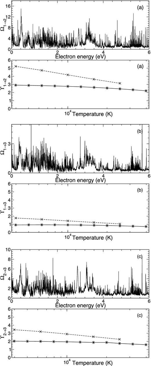
The collision strengths, (a) Ω1 → 2, (b) Ω1 → 3 and (c) Ω2 → 3 presented as a function of electron energy in eV. Also presented are the corresponding effective collision strengths as a function of temperature in K. Solid black lines with stars are the current data set and the dashed line with crosses represent the results from Storey & Sochi (2016).
Comparison of the effective collision strengths are made for each transition with the work of Storey & Sochi (2016) and good agreement is found for all temperatures above 10 000 K. For temperatures below this value the two calculations deviate somewhat, most probably due to the differing resonance profiles converging on to differing threshold positions. The present calculation has shifted the thresholds to lie in their exact observed positions listed in Table 1. In Fig. 6 we present the effective collision strengths for some higher lying transitions, the 3d74F9/2–3d72G9/2 (1 → 8), 3d72P1/2–3d72H9/2 (11 → 13) and 3d72G7/2–3d72H9/2 (9 → 13). Excellent agreement is evident for all three transitions when a comparison is made with the data of Storey & Sochi (2016) across all temperatures where a comparison is possible. The collision strengths and effective collision strengths for all 42 486 forbidden and allowed lines are available from the authors on request but we present in Table 4 the effective collision strengths for all transitions among the lowest 11 3d7 fine-structure levels across nine temperatures of astrophysical importance.1
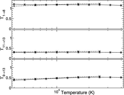
The effective collision strengths, ϒ1 → 8 (top), ϒ11 → 13 (middle) and ϒ9 → 13 (bottom), presented as a function of temperature in K (bottom). Solid black lines with stars are the current data set and the dashed line with crosses represent the results from Storey & Sochi (2016).
Effective collision strengths as defined by equation (5) are presented between an upper (j) and lower state (i), across a range of nine temperatures (K), 3800 < T < 25 100 K. We have denoted (a) ≡ ×10a.
| log T (K) | ||||||||||
|---|---|---|---|---|---|---|---|---|---|---|
| i | j | 3.6 | 3.7 | 3.8 | 3.9 | 4 | 4.1 | 4.2 | 4.3 | 4.4 |
| 1 | 2 | 2.92(0) | 2.90(0) | 2.86(0) | 2.82(0) | 2.77(0) | 2.70(0) | 2.63(0) | 2.54(0) | 2.44(0) |
| 1 | 3 | 9.24(−1) | 9.36(−1) | 9.41(−1) | 9.37(−1) | 9.26(−1) | 9.06(−1) | 8.79(−1) | 8.45(−1) | 8.06(−1) |
| 2 | 3 | 2.02(0) | 2.01(0) | 1.99(0) | 1.97(0) | 1.94(0) | 1.91(0) | 1.86(0) | 1.81(0) | 1.74(0) |
| 1 | 4 | 3.17(−1) | 3.23(−1) | 3.26(−1) | 3.25(−1) | 3.21(−1) | 3.13(−1) | 3.03(−1) | 2.90(−1) | 2.75(−1) |
| 2 | 4 | 7.46(−1) | 7.65(−1) | 7.77(−1) | 7.80(−1) | 7.76(−1) | 7.64(−1) | 7.43(−1) | 7.17(−1) | 6.85(−1) |
| 3 | 4 | 1.42(0) | 1.42(0) | 1.42(0) | 1.42(0) | 1.40(0) | 1.39(0) | 1.36(0) | 1.32(0) | 1.28(0) |
| 1 | 5 | 1.16(0) | 1.16(0) | 1.17(0) | 1.19(0) | 1.20(0) | 1.21(0) | 1.21(0) | 1.20(0) | 1.19(0) |
| 2 | 5 | 8.11(−1) | 8.03(−1) | 8.02(−1) | 8.07(−1) | 8.13(−1) | 8.17(−1) | 8.15(−1) | 8.05(−1) | 7.89(−1) |
| 3 | 5 | 5.72(−1) | 5.60(−1) | 5.53(−1) | 5.51(−1) | 5.50(−1) | 5.48(−1) | 5.43(−1) | 5.33(−1) | 5.19(−1) |
| 4 | 5 | 3.68(−1) | 3.51(−1) | 3.37(−1) | 3.27(−1) | 3.20(−1) | 3.13(−1) | 3.06(−1) | 2.98(−1) | 2.88(−1) |
| 1 | 6 | 4.84(−1) | 4.82(−1) | 4.84(−1) | 4.90(−1) | 4.95(−1) | 4.98(−1) | 4.97(−1) | 4.91(−1) | 4.82(−1) |
| 2 | 6 | 5.54(−1) | 5.52(−1) | 5.53(−1) | 5.56(−1) | 5.60(−1) | 5.61(−1) | 5.58(−1) | 5.52(−1) | 5.41(−1) |
| 3 | 6 | 4.55(−1) | 4.51(−1) | 4.51(−1) | 4.54(−1) | 4.57(−1) | 4.59(−1) | 4.57(−1) | 4.52(−1) | 4.44(−1) |
| 4 | 6 | 2.92(−1) | 2.88(−1) | 2.89(−1) | 2.92(−1) | 2.96(−1) | 3.00(−1) | 3.02(−1) | 3.00(−1) | 2.96(−1) |
| 5 | 6 | 6.14(−1) | 6.15(−1) | 6.21(−1) | 6.31(−1) | 6.44(−1) | 6.59(−1) | 6.73(−1) | 6.82(−1) | 6.87(−1) |
| 1 | 7 | 1.86(−1) | 1.85(−1) | 1.85(−1) | 1.86(−1) | 1.87(−1) | 1.86(−1) | 1.84(−1) | 1.81(−1) | 1.76(−1) |
| 2 | 7 | 2.03(−1) | 2.03(−1) | 2.06(−1) | 2.10(−1) | 2.15(−1) | 2.18(−1) | 2.19(−1) | 2.18(−1) | 2.14(−1) |
| 3 | 7 | 2.34(−1) | 2.36(−1) | 2.39(−1) | 2.43(−1) | 2.48(−1) | 2.51(−1) | 2.53(−1) | 2.52(−1) | 2.48(−1) |
| 4 | 7 | 2.19(−1) | 2.20(−1) | 2.22(−1) | 2.26(−1) | 2.29(−1) | 2.31(−1) | 2.32(−1) | 2.31(−1) | 2.28(−1) |
| 5 | 7 | 2.43(−1) | 2.45(−1) | 2.49(−1) | 2.56(−1) | 2.65(−1) | 2.75(−1) | 2.85(−1) | 2.93(−1) | 2.98(−1) |
| 6 | 7 | 2.73(−1) | 2.72(−1) | 2.72(−1) | 2.74(−1) | 2.76(−1) | 2.79(−1) | 2.81(−1) | 2.83(−1) | 2.82(−1) |
| 1 | 8 | 1.22(0) | 1.20(0) | 1.19(0) | 1.19(0) | 1.19(0) | 1.19(0) | 1.19(0) | 1.19(0) | 1.18(0) |
| 2 | 8 | 7.27(−1) | 7.14(−1) | 7.06(−1) | 7.02(−1) | 6.99(−1) | 6.98(−1) | 6.96(−1) | 6.92(−1) | 6.86(−1) |
| 3 | 8 | 3.85(−1) | 3.76(−1) | 3.70(−1) | 3.65(−1) | 3.62(−1) | 3.59(−1) | 3.55(−1) | 3.51(−1) | 3.45(−1) |
| 4 | 8 | 1.75(−1) | 1.69(−1) | 1.65(−1) | 1.60(−1) | 1.57(−1) | 1.53(−1) | 1.50(−1) | 1.46(−1) | 1.43(−1) |
| 5 | 8 | 3.24(−1) | 3.18(−1) | 3.11(−1) | 3.07(−1) | 3.04(−1) | 3.02(−1) | 3.01(−1) | 3.00(−1) | 2.98(−1) |
| 6 | 8 | 1.56(−1) | 1.51(−1) | 1.47(−1) | 1.43(−1) | 1.41(−1) | 1.40(−1) | 1.39(−1) | 1.38(−1) | 1.37(−1) |
| 7 | 8 | 5.48(−2) | 5.20(−2) | 4.93(−2) | 4.70(−2) | 4.51(−2) | 4.36(−2) | 4.24(−2) | 4.14(−2) | 4.03(−2) |
| 1 | 9 | 3.16(−1) | 3.10(−1) | 3.06(−1) | 3.05(−1) | 3.05(−1) | 3.04(−1) | 3.03(−1) | 3.01(−1) | 2.97(−1) |
| 2 | 9 | 5.02(−1) | 4.99(−1) | 4.99(−1) | 5.01(−1) | 5.05(−1) | 5.08(−1) | 5.11(−1) | 5.12(−1) | 5.10(−1) |
| 3 | 9 | 5.33(−1) | 5.29(−1) | 5.29(−1) | 5.31(−1) | 5.34(−1) | 5.37(−1) | 5.40(−1) | 5.41(−1) | 5.39(−1) |
| 4 | 9 | 4.29(−1) | 4.27(−1) | 4.26(−1) | 4.27(−1) | 4.29(−1) | 4.32(−1) | 4.33(−1) | 4.34(−1) | 4.32(−1) |
| 5 | 9 | 1.53(−1) | 1.46(−1) | 1.41(−1) | 1.37(−1) | 1.36(−1) | 1.36(−1) | 1.36(−1) | 1.37(−1) | 1.36(−1) |
| 6 | 9 | 1.72(−1) | 1.66(−1) | 1.62(−1) | 1.58(−1) | 1.56(−1) | 1.56(−1) | 1.55(−1) | 1.55(−1) | 1.55(−1) |
| 7 | 9 | 1.09(−1) | 1.06(−1) | 1.04(−1) | 1.02(−1) | 1.01(−1) | 9.99(−2) | 9.95(−2) | 9.92(−2) | 9.86(−2) |
| 8 | 9 | 1.29(0) | 1.27(0) | 1.26(0) | 1.26(0) | 1.27(0) | 1.28(0) | 1.29(0) | 1.29(0) | 1.28(0) |
| 1 | 10 | 3.06(−1) | 3.04(−1) | 3.04(−1) | 3.03(−1) | 3.03(−1) | 3.02(−1) | 3.00(−1) | 2.99(−1) | 2.97(−1) |
| 2 | 10 | 2.76(−1) | 2.79(−1) | 2.82(−1) | 2.86(−1) | 2.88(−1) | 2.89(−1) | 2.87(−1) | 2.83(−1) | 2.78(−1) |
| 3 | 10 | 2.05(−1) | 2.09(−1) | 2.13(−1) | 2.18(−1) | 2.21(−1) | 2.21(−1) | 2.20(−1) | 2.16(−1) | 2.10(−1) |
| 4 | 10 | 1.29(−1) | 1.32(−1) | 1.36(−1) | 1.40(−1) | 1.43(−1) | 1.43(−1) | 1.42(−1) | 1.39(−1) | 1.34(−1) |
| 5 | 10 | 2.85(−1) | 2.84(−1) | 2.86(−1) | 2.89(−1) | 2.92(−1) | 2.95(−1) | 2.95(−1) | 2.93(−1) | 2.89(−1) |
| 6 | 10 | 2.29(−1) | 2.27(−1) | 2.27(−1) | 2.29(−1) | 2.31(−1) | 2.32(−1) | 2.31(−1) | 2.29(−1) | 2.25(−1) |
| 7 | 10 | 9.14(−2) | 9.23(−2) | 9.39(−2) | 9.56(−2) | 9.69(−2) | 9.75(−2) | 9.72(−2) | 9.60(−2) | 9.40(−2) |
| 8 | 10 | 4.12(−1) | 4.06(−1) | 4.01(−1) | 3.99(−1) | 3.99(−1) | 4.00(−1) | 4.03(−1) | 4.07(−1) | 4.09(−1) |
| 9 | 10 | 3.20(−1) | 3.17(−1) | 3.17(−1) | 3.20(−1) | 3.26(−1) | 3.34(−1) | 3.42(−1) | 3.47(−1) | 3.50(−1) |
| 1 | 11 | 8.09(−2) | 8.03(−2) | 8.01(−2) | 8.02(−2) | 8.05(−2) | 8.08(−2) | 8.09(−2) | 8.08(−2) | 8.03(−2) |
| 2 | 11 | 1.09(−1) | 1.10(−1) | 1.11(−1) | 1.11(−1) | 1.12(−1) | 1.12(−1) | 1.12(−1) | 1.11(−1) | 1.09(−1) |
| 3 | 11 | 1.16(−1) | 1.19(−1) | 1.22(−1) | 1.26(−1) | 1.28(−1) | 1.29(−1) | 1.28(−1) | 1.27(−1) | 1.24(−1) |
| 4 | 11 | 9.23(−2) | 9.71(−2) | 1.02(−1) | 1.07(−1) | 1.11(−1) | 1.13(−1) | 1.13(−1) | 1.11(−1) | 1.08(−1) |
| 5 | 11 | 7.49(−2) | 7.54(−2) | 7.66(−2) | 7.83(−2) | 8.00(−2) | 8.14(−2) | 8.23(−2) | 8.23(−2) | 8.14(−2) |
| 6 | 11 | 8.77(−2) | 8.98(−2) | 9.27(−2) | 9.61(−2) | 9.93(−2) | 1.02(−1) | 1.04(−1) | 1.04(−1) | 1.03(−1) |
| 7 | 11 | 6.77(−2) | 6.93(−2) | 7.18(−2) | 7.45(−2) | 7.70(−2) | 7.88(−2) | 7.96(−2) | 7.94(−2) | 7.81(−2) |
| 8 | 11 | 1.98(−1) | 1.90(−1) | 1.85(−1) | 1.81(−1) | 1.79(−1) | 1.78(−1) | 1.78(−1) | 1.79(−1) | 1.79(−1) |
| 9 | 11 | 2.06(−1) | 2.01(−1) | 1.99(−1) | 1.99(−1) | 2.00(−1) | 2.03(−1) | 2.07(−1) | 2.11(−1) | 2.14(−1) |
| 10 | 11 | 3.32(−1) | 3.24(−1) | 3.19(−1) | 3.17(−1) | 3.17(−1) | 3.17(−1) | 3.16(−1) | 3.14(−1) | 3.09(−1) |
3.3 Line ratios
Combining the electron-impact excitation rates with the decay rates (A-values), it is possible to investigate important infrared and visible line ratios. For simplicity and purpose of this study, we neglect the recombination and ionization process from the neighbouring ion stages and focus on the populating mechanisms solely of Co iii. Assuming local thermal equilibrium and detailed balance, we can derive the collisional radiative modelling approach detailed in (Griffin et al. 1997). We can therefore investigate selected transitions that have been suggested as temperature or density diagnostics.
We present in Table 5 a comparison of emissivities (ρij) between our current results, and those from Storey & Sochi (2016) for particular transitions at electron densities Ne = 104 cm−3 and Ne = 107 cm−3. The emissivities are calculated relative to the H β line [see equation (1) in Storey & Sochi (2016)], where the effective recombination coefficients |$\bar{\alpha }_{4\rightarrow 2}$| can be found in Hummer & Storey (1987) and Storey & Hummer (1995). The wavelengths are those from National Institute of Standards and Technology (NIST) and we use our current set of A-values. In general there is excellent agreement for all emissivities considered with the major outlier ρ1 → 2 found to be around 30 per cent at Ne = 104 cm−3. This is evident from the strong ϒ1 → 2 from Fig. 5(a) at T = 104 K. By replacing this one effective collision strength to ϒ1 → 2(T = 10 000) = 4.18, then the ρ1 → 2 differences are within a much more agreeable 8 per cent. A similar argument follows for the large differences in the ρ2 → 3 at low electron density.
Emissivities relative to H β for a select number of transitions. The results are from our Present calculation and those presented in Storey & Sochi (2016) for two electron densities at one temperature, T = 10 000 K.
| ρ (Ne = 104) | ρ (Ne = 107) | |||
|---|---|---|---|---|
| i − j | Present | Storey | Present | Storey |
| 1 – 2 | 4.06 × 10⁴ | 5.85 × 10⁴ | 6.69 × 10² | 7.49 × 10² |
| 1 – 5 | 2.24 × 10⁴ | 2.27 × 10⁴ | 2.19 × 10³ | 2.62 × 10³ |
| 1 – 8 | 2.89 × 10⁴ | 2.83 × 10⁴ | 1.15 × 10⁴ | 1.26 × 10⁴ |
| 2 – 3 | 8.79 × 10³ | 1.26 × 10⁴ | 2.14 × 10² | 2.17 × 10² |
| 2 – 5 | 5.89 × 10³ | 5.83 × 10³ | – | – |
| 2 – 6 | 6.87 × 10³ | 6.93 × 10³ | 7.70 × 10² | 9.23 × 10² |
| 2 – 8 | 8.65 × 10³ | 8.47 × 10³ | 3.45 × 10³ | 3.78 × 10³ |
| 2 – 9 | – | – | 3.54 × 10³ | 3.82 × 10³ |
| 2 – 13 | 3.84 × 10³ | 4.07 × 10³ | 5.15 × 10³ | 5.39 × 10³ |
| 3 – 4 | 1.49 × 10³ | 1.94 × 10³ | 3.20 × 101 | 3.26 × 101 |
| 3 – 6 | 3.83 × 10³ | 3.91 × 10³ | – | – |
| 3 – 9 | – | – | 2.56 × 10³ | 2.74 × 10³ |
| 3 – 15 | – | – | 2.02 × 10³ | 2.38 × 10³ |
| 4 – 15 | – | – | 1.04 × 10³ | 1.24 × 10³ |
| 8 – 12 | 3.90 × 10³ | 3.82 × 10³ | – | – |
| 8 – 14 | – | – | 5.36 × 10² | 7.49 × 10² |
![The line ratio [0.66 μm]/[0.69 μm] as a function of electron density (cm−3). The dashed curve is the lowest temperature, T = 3980 K. The remaining solid black curves are for temperatures T = 5010, 6310, and 7940 K for decreasing line ratio.](https://oup.silverchair-cdn.com/oup/backfile/Content_public/Journal/mnras/462/3/10.1093_mnras_stw1843/2/m_stw1843fig7.jpeg?Expires=1750367654&Signature=t4c9HarAj8SvOwSsMOqElTC8thUqQ2sTCwF-3RmxTGVnZOAUPYa1VSAvuT9ehMyudZU4-aVT9Ug4abJR7DTICj6r8dfEE9Uv7mS6Z6-Ew-jcsRh92f34h9z2ETiAe6Ep9xQwmk2LeXE0nTch0e2FbbFkqvwNswGdFvMRbdsOlIFSRKLX4yuuVRvSWNzczxH7uy5UiGUOSx61QIHGkgOVhpWlERfzJH1gr7hApkJ2dc1u83TH-lrYRBCFefYR1PjwU-gv340BjlxDRi5nafPhLnEZhckv4jjRbtm9QcR-M14Bbiy8n8XikIdEvqPx2JUL~2m-zAjULsgFx6bOzU5HEg__&Key-Pair-Id=APKAIE5G5CRDK6RD3PGA)
The line ratio [0.66 μm]/[0.69 μm] as a function of electron density (cm−3). The dashed curve is the lowest temperature, T = 3980 K. The remaining solid black curves are for temperatures T = 5010, 6310, and 7940 K for decreasing line ratio.
We plot all three line ratios above in Fig. 8 as a function of electron temperature. The red dashed curve is the lowest electron density in each subfigure, Ne = 102 cm−3, and the remaining solid curves correspond to Ne = 104, 105, and 106 cm−3. Each line ratio is a varying function of increasing temperature across the range of interest. The line ratios for the two lowest densities are generally unchanged, and therefore they provide useful diagnostics for this density range. As Ne = 105 cm−3 and beyond, the line ratio begins to diverge, and becomes constant again for even larger densities.
![The line ratio [11.88 μm]/[0.66 μm] (left), [11.88 μm]/[0.59 μm] (middle), and [11.88 μm]/[0.62 μm] (right) as a function of electron temperature (K). The red, dashed curve is the lowest density, Ne = 102 cm−3. The remaining solid black curves are for densities Ne = 104 cm−3, 105, and 106 cm−3 for decreasing line ratio.](https://oup.silverchair-cdn.com/oup/backfile/Content_public/Journal/mnras/462/3/10.1093_mnras_stw1843/2/m_stw1843fig8.jpeg?Expires=1750367654&Signature=h5ULvD~FmXKAT5VWlQKBuOBl4BdiNRa0pvXu6iCIJnZDB7rItO2E1raboz0TVFE4Sjv7hhPVMtsXCwiCrU7z0PE-YCbrnMkLE-fswMSsT6cGijM6cRhzR3shLgxavGgVxDFNUkZAIYjtC7a2CIhAMaN33OWOyboWv~jATyN~-WN2wzD-TaUcBR0y-b6leRjxTdtxG1R6rXU45Lo7r9vsGIb7a0DidsXsv0cjPEI5qhlvMOxeQ96JuFtC~AkTS5WLTNAfMGJfDtNmpCywO6xJq4aykHJPPFf0FXQ58xRXNmoSiVE~4ik1O3S63z6hZmWc~0K7Mh670ObhkwhzJHHzkg__&Key-Pair-Id=APKAIE5G5CRDK6RD3PGA)
The line ratio [11.88 μm]/[0.66 μm] (left), [11.88 μm]/[0.59 μm] (middle), and [11.88 μm]/[0.62 μm] (right) as a function of electron temperature (K). The red, dashed curve is the lowest density, Ne = 102 cm−3. The remaining solid black curves are for densities Ne = 104 cm−3, 105, and 106 cm−3 for decreasing line ratio.
4 CONCLUSION
In this paper, we present an extensive set of atomic data for the photoionization of Co ii and the electron-impact excitation of Co iii. Initially we have exploited the computer code grasp0 to obtain a description of the atomic wavefunctions and generate energy levels for the 292 fine-structure bound target states and the corresponding A-values for transitions between these levels. Furthermore, the darc computer package has been employed to extend the problem to include photon and electron interactions. We present statistically weighted, level-resolved ground and metastable photoionization cross-sections for the Co ii ion as well as collision strengths and Maxwellian averaged effective collision strengths describing the electron-impact excitation of the Co iii ion. Comparisons are made with other works where possible and good agreement is found where a comparison is available. The reliability of the atomic data presented has been rigorously tested through a variety of means, such as the sophistication of the current calculations where great care has been taken to ensure the inclusion of important correlation and configuration-interaction in the wavefunction expansions. In addition the complex resonance structures in the cross-sections (photoionization and excitation) have been accurately resolved through a series of calculations incorporating mesh sizes with finer and finer energy increments. A proper consideration was also taken of the contributions from the high partial waves to ensure convergence of the collision strengths for the allowed transitions in particular (which are not presented in this work). A conclusive assessment of the accuracy of the presented Maxwellian averaged collision strengths will necessarily come from any subsequent astrophysical or diagnostic application. In Section 3.3 the electron-impact excitation rates were combined with the decay rates (A-values) to investigate important infrared and visible line ratios. During this process we were able to identify useful transitions that could be used as temperature and/or density sensitive diagnostic lines.
The work conducted has been supported by STFC through the grant ST/K000802/1. The authors would also like to acknowledge time on the Stuttgart, Hazelhen machine under the PAMOP (44009) project where all calculations have been performed.
The results are also in the form of an adf04 file on http://open.adas.ac.uk and on QUB pure.
REFERENCES
