


Abstract
We use a sample of 1669 quasars (r < 20.15, 3.6 < z < 4.0) from the Baryon Oscillation Spectroscopic Survey to study the intrinsic shape of their continuum and the Lyman continuum photon escape fraction (fesc,q), estimated as the ratio between the observed flux and the expected intrinsic flux (corrected for the intergalactic medium absorption) in the wavelength range 865–885 Å rest frame. Modelling the intrinsic quasar (QSO) continuum shape with a power law, Fλ ∝ λ−γ, we find a median γ = 1.30 (with a dispersion of 0.38, no dependence on the redshift and a mild intrinsic luminosity dependence) and a mean fesc,q = 0.75 (independent of the QSO luminosity and/or redshift). The fesc,q distribution shows a peak around zero and a long tail of higher values, with a resulting dispersion of 0.7. If we assume for the QSO continuum a double power-law shape (also compatible with the data) with a break located at λbr = 1000 Å and a softening Δγ = 0.72 at wavelengths shorter than λbr, the mean fesc,q rises to 0.82. Combining our γ and fesc,q estimates with the observed evolution of the active galactic nucleus (AGN) luminosity function (LF), we compute the AGN contribution to the UV ionizing background (UVB) as a function of redshift. AGN brighter than one-tenth of the characteristic luminosity of the LF are able to produce most of it up to z ∼ 3, if the present sample is representative of their properties. At higher redshifts, a contribution of the galaxy population is required. Assuming an escape fraction of Lyman continuum photons from galaxies between 5.5 and 7.6 per cent, independent of the galaxy luminosity and/or redshift, a remarkably good fit to the observational UVB data up to z ∼ 6 is obtained. At lower redshift, the extrapolation of our empirical estimate agrees well with recent UVB observations, dispelling the so-called Photon Underproduction Crisis.
1 INTRODUCTION
After more than 35 years (Sargent et al. 1980), the issue of the sources driving the reionization of the hydrogen in the Universe and keeping it ionized afterwards does not appear to be settled. It is commonplace that galaxies should be able to produce the bulk of the UV emissivity at high redshift (see, for example, Robertson et al. 2015), but the active galactic nucleus (AGN) population is also proposed as a relevant or dominant contributor (Giallongo et al. 2015; Madau & Haardt 2015, see also Fontanot, Cristiani & Vanzella 2012; Haardt & Salvaterra 2015, for different views).
A direct measurement of the 1–4 Ryd photons escaping the various types of sources is unpractical at z ≳ 4.5, due to the reduced mean free path of these photons in the intergalactic medium (IGM). At lower redshift, direct observations of galaxies, after accounting for the statistical contamination of interlopers, have in general provided upper limits in the fraction of ionizing photons, produced by young stars, that are able to escape to the IGM (fesc, g, see Vanzella et al. 2012). These limits tend to be significantly lower than ∼20 per cent required at z ≃ 7 to re-ionize the Universe with galaxies only (Bouwens et al. 2011; Haardt & Madau 2012), and an increasing fesc, g with decreasing luminosity [possibly with a steep faint end of the luminosity function (LF)] has been invoked to circumvent this shortcoming (Fontanot et al. 2014). The corresponding fesc,q for QSOs is typically assumed to be about 100 per cent.
In this paper, we aim to obtain a precise measurement of the QSO contribution to the cosmic UV background in the range 3.6 < z < 4.0, where the QSO LF is well determined and the IGM transmission not too low. Our strategy is first to estimate the intrinsic QSO continuum shape up to 4 Ryd (Section 3), then we compare the fitted spectral energy distribution (SED) with the observed flux (corrected for the effect of the IGM absorption with the model of Inoue et al. 2014), and finally we compute the fraction of UV photons below the Lyman limit escaping to the IGM (fesc,q, Section 4). We take advantage of the large samples of QSOs that can be extracted from the Sloan Digital Sky Survey (SDSS) to investigate possible correlations with the luminosity and redshift. Finally, we combine this information with the knowledge of the QSO LF to synthesize the global production of ionizing photons from QSOs at various redshifts and compare it with measurements of the UV ionizing background (UVB) obtained from observations of the IGM (Section 5). In this way it is possible to assess how much room is left/needed for the contribution of galaxies at the various cosmic epochs and where preferably to look for it.
2 DATA SAMPLE
The Baryon Oscillation Spectroscopic Survey (BOSS; Dawson et al. 2013) provides a large data base of quasar spectra. The quasar target selection used in BOSS is summarized in Ross et al. (2012), and combines various targeting methods described in Yèche et al. (2010), Kirkpatrick et al. (2011) and Bovy et al. (2011).
We have extracted from the 11th Data Release the quasars in the redshift range 3.6 < z ≤ 4.0 with magnitudes brighter than r = 20.15. The lower limit in the redshift interval is due to a known selection effect in the BOSS survey outlined by Prochaska, Worseck & O'Meara (2009): the QSOs found in the range 3 < z < 3.6 are selected with a bias against having (u − g) < 1.5, which translates into a tendency to select sightlines with strong Lyman limit absorption. On the other hand, the analysis by Prochaska et al. (2009) shows that beyond zem = 3.6 very few QSOs are predicted to have such a blue (u − g) < 1.5 colour, removing the possibility of a bias. We are therefore confident that the sample used can be considered statistically complete and representative of the bright (MV ≲ −27.5) QSO population. In particular, for the discussion to follow, we note that Broad Absorption Line (BAL) objects are included in the present sample. The upper limit in the redshift range of the present sample, z = 4.0, is due to the requirement to have the observed spectra reaching the rest-frame wavelength of 2000 Å in order to have a sufficiently extended domain to estimate the intrinsic QSO continuum shape.
The SED of each quasar has been adjusted using a linear multiplicative slope (in magnitude) in order to match the g, r, i, z magnitudes from the SDSS photometric catalogue and then corrected for galactic extinction according to the maps of Schlafly & Finkbeiner (2011) and the average Milky Way extinction curve of Cardelli, Clayton & Mathis (1989).
All the spectra have been visually inspected and their systemic redshifts calculated. We have adopted the offsets of −310 km s−1 and +177 km s−1, respectively assigned to the C iv 1549 and Si iv 1398 lines (Tytler & Fan 1992) to derive the systemic redshift. A small fraction (≲1 per cent) of spectra showing problems in terms of the observed S/N ratio have been excluded from the subsequent analysis. The resulting sample consists of 1669 objects and the associated redshift distribution is shown in Fig. 1. The number of QSOs declines from about 300 per Δz = 0.05 bin in the interval 3.6 < z < 3.7 to about 100 at z ≃ 4, following the general trend of the BOSS survey. The distribution of the recomputed redshifts shows a small systematic difference with respect to the SDSS data, 〈Δz〉 = 〈zcorr − zSDSS〉 = −0.008, with a dispersion of 0.012.
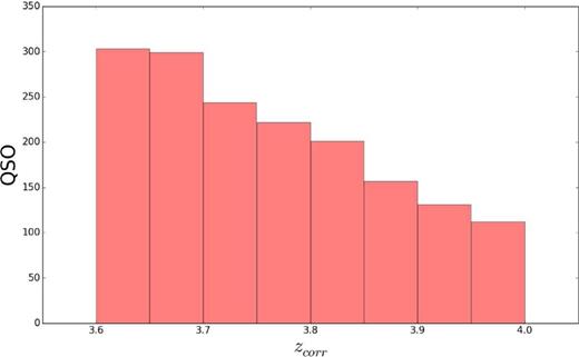
Redshift distribution of the QSOs in the present sample shown in bins of Δz = 0.05. zcorr on the x-axis indicates the redshift estimated according to the procedure described in Section 2.
3 ESTIMATE OF THE QSO SED
In order to estimate the QSO production of UV ionizing photons it is necessary to model their intrinsic spectral shape. Customarily, this is achieved by fitting a power law, Fλ ∝ λ−γ, in the region redward of the Lyman α emission, selecting windows free of emission lines and extrapolating it in the region blueward of the Lyman α (e.g. Fig. 2). Previous works by Zheng et al. (1997), Telfer et al. (2002), Shull, Stevans & Danforth (2012) and Stevans et al. (2014) at relatively low redshift (z ≲ 1.5), where the IGM absorption is minimized, have identified a break in the spectral distribution with a softening of the slope at wavelengths shorter than λbr ∼ 1000 Å.
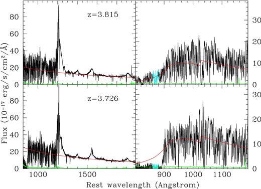
Two illustrative cases for the estimate of the continuum power law and the escape fraction. The upper panels show a QSO of redshift 3.815 with a fesc,q ∼ 1, the lower panels a QSO of redshift 3.726 with a fesc,q ∼ 0. Left-hand column: the two spectra are plotted in black. Note that the region blueward of the Lyman α has been divided by the average transmission of the IGM estimated (see Section 4) according to Inoue et al. (2014) in order to show where the average continuum should be located. The green line shows the uncertainty of the flux. The red line shows the fitted power-law continuum. Right-hand column: the two observed spectra are plotted in black, the expected position of the power-law continuum multiplied by the average IGM transmission is in red and the uncertainty of the observed flux in green. The cyan portion of the spectrum is the region where the escape fraction of the UV photons produced by the QSO has been estimated.
In the following, we have chosen to fit the continuum spectrum of each quasar both with a single and with a broken power law. In both the cases, five windows, listed in Table 1, have been used for the fit as emission-line-free regions. In the case of the broken power-law fit, we have imposed a flattening in the spectral slope blueward of 1000 Å of Δγ = 0.72 with respect to the power law at longer wavelengths, as reported by Stevans et al. (2014). Pixels affected by absorption lines have been iteratively rejected on the basis of a 3σ k-clipping. We have checked that the results are not sensitive to the particular choice of the windows.
Regions used for the continuum fitting.
| Region | Start | End |
|---|---|---|
| Rest-frame wavelength | ||
| (Å) | ||
| 1 | 1990 | 2020 |
| 2 | 1690 | 1700 |
| 3 | 1440 | 1465 |
| 4 | 1322 | 1329 |
| 5 | 1284 | 1291 |
| Region | Start | End |
|---|---|---|
| Rest-frame wavelength | ||
| (Å) | ||
| 1 | 1990 | 2020 |
| 2 | 1690 | 1700 |
| 3 | 1440 | 1465 |
| 4 | 1322 | 1329 |
| 5 | 1284 | 1291 |
As a check of the goodness of the assumptions, we have stacked all the spectra after dividing them by the continuum slope and by the expected mean transmission of the IGM according to the computation by Inoue et al. (2014). For the IGM transmission, we have used the numerical tables kindly provided by the authors, which are slightly more accurate than the analytical approximation, especially in the region between the Lyman β and the Lyman limit. The result is shown in Fig. 3. The continuum-normalized average flux, corrected by the IGM absorption, in a true-continuum window of the Lyman α forest (1080 < λ < 1120, see Shull et al. 2012 and Stevans et al. 2014) turns out to be 1.01 ± 0.04 (see Fig. 3). It is also remarkable to see the correspondence between the emission bumps observed in the Lyman forest by us and by Shull et al. (2012) and Stevans et al. (2014), in particular around 1125 Å (Fe iii) and 1070 Å(N ii, He ii).

Stacked spectrum of the 1669 BOSS QSOs, after dividing each QSO spectrum by the average IGM transmission and by the estimated individual power-law continuum. Upper panel: 1000–2000 Å rest-frame wavelength range. Lower panel: 850–1020 Å wavelength range. In the lower panel, the lower black line corresponds to a single power-law continuum, while the upper blue line to the broken power-law fitting (see the text). The region 865–885 Å rest frame, where the escape fraction has been measured (see Section 4), is shown in red.
We have then analysed the ensemble properties of the quasars in our sample. The median (mean) spectral index of the population for the single power-law case (and for the region with λ > 1000 Å for the broken power law) is γ = 1.30 (1.24), with a dispersion of 0.38, computed as half of the difference between the 84.13 and 15.87 percentiles (Fig. 5). A Kolmogorov–Smirnov (KS) test on the two samples above and below redshift z = 3.8 does not show any significant difference in the two distributions (see also Figs 4 and 5). We have checked that selecting QSOs with 3.4 < z < 3.6 (and r < 20.15), we would obtain a value of γ significantly lower than the one we measure in the range 3.6 < z ≤ 4.0, confirming the above-mentioned bias found by Prochaska et al. (2009). The dependence of the spectral index on the SDSS r magnitude has also been analysed by splitting the sample in two halves: r ≤ 19.69 and r > 19.69. The corresponding median spectral indices turn out to be γ = 1.36 and γ = 1.22, respectively, with fainter objects generally characterized by ‘redder’ spectral indices. A KS test rejects with a high significance the hypothesis that the two subsamples have the same distribution function. We interpret this effect as a property of the SEDs of the QSOs analysed, rather than a bias introduced by the fitting procedure, since a corresponding difference is present in the measured colours of the QSOs: the average (r − i) is 0.115 for objects brighter than r = 19.69 and 0.138 for the fainter ones.
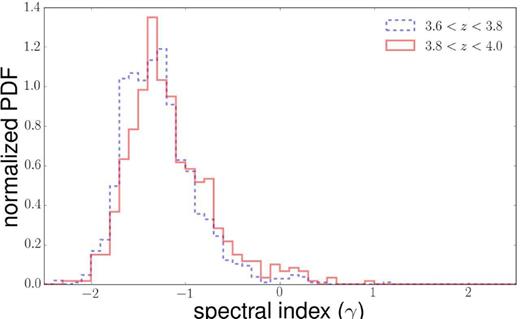
Normalized probability distributions of the spectral index γ for QSOs in the redshift interval 3.6 < z ≤ 3.8 (blue dashed line) and 3.8 < z ≤ 4.0 (red continuous line).
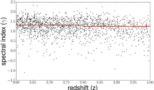
Distribution of the spectral indices of the continuum power law of the QSO spectra as a function of the redshift. The median values in the intervals 3.6 < z ≤ 3.8, 3.8 < z ≤ 4.0, are shown as continuous red segments.
The median (mean) value of the spectral index for the full sample, γ = 1.30 (1.24), can be compared with the results based on Hubble Space Telescope (HST) Cosmic Origins Spectrograph (COS) data at z < 1.5 by Shull et al. (2012), who find γ = 1.32 ± 0.14 and Stevans et al. (2014), who measure γ = 1.17 ± 0.09. Telfer et al. (2002) with a similar approach and wavelength windows to ours, at 〈z〉 = 1.17 find a γ = 1.31 ± 0.06 with HST Faint Object Spectrograph (FOS), Goddard High-Resolution Spectrograph (GHRS) and Space Telescope Imaging Spectrograph (STIS) data.
4 The average escape fraction of the QSO population at 3.6 < z ≤ 4.0
The fraction of the UV ionizing photons produced by each QSO leaking to the IGM has been estimated by dividing the observed average flux in the region 865–885 Å rest frame by the expected average flux in the same region, as estimated either with the single or with the broken power law, convolved with the average transmission of the IGM at the given redshift (Inoue et al. 2014). The interval 865–885 Å has been chosen since it is expected to be a ‘true continuum’ window (see fig. 6 in Shull et al. 2012 and fig. 5 in Stevans et al. 2014). Besides, it represents a convenient compromise: on the one hand, at wavelengths close to the Lyman edge the measurement can be affected by errors in the determination of the emission redshift of the QSO; on the other hand, the IGM transmission is progressively decreasing at shorter and shorter wavelengths with a consequent increase of the measurement uncertainty. The resulting value of the fesc,q has been checked to be largely independent of the specific choice of the limits of the interval.
The estimated fesc,q is an effective escape fraction, i.e. is expected to include the escape fraction of the UV photons from the QSO host galaxy and all the extra absorption due to clustered neutral hydrogen in the vicinity of the QSO that is not accounted for in the model of Inoue et al. (2014) which applies to the average, intervening IGM.
The average escape fraction in the redshift interval 3.6 < z < 4.0, measured on the ensemble of 1669 objects of our sample turns out to be fesc,q = 0.75 and fesc,q = 0.82 in the case of the single and broken power law, respectively. As shown in Figs 6 and 7, a rather large dispersion is observed, 0.7, computed as half of the difference between the 84.13 and 15.87 percentiles, in a kind of bimodal distribution with a narrower peak around the value zero and a larger dispersion around the value 1. In each object, fesc,q is computed by comparing the observed flux shortward of the Lyman edge and the expected flux on the basis of an average correction for the IGM absorption. It is not surprising, therefore, that for some objects our measured fesc,q turns out to be larger than 1 – besides the measurement errors – due to lines of sight with an actual transmission larger than the average estimate from the Inoue et al. (2014) computation.

Escape fraction measured in the QSO spectra as a function of the redshift. The mean values in the intervals 3.6 < z ≤ 3.8 and 3.8 < z ≤ 4.0 are shown as continuous red segments, with the dispersion estimated as half of the difference between the 84.15 and 15.87 percentiles.

Normalized probability distributions of the escape fraction fesc,q for QSOs in the redshift interval 3.6 < z ≤ 4.0. The black continuous line shows the full sample. The red dashed line corresponds to objects with r ≤ 19.69, while the blue dashed line refers to objects with r > 19.69.
Fig. 6 shows the escape fraction measured in the QSO spectra as a function of the redshift. In the intervals 3.6 < z ≤ 3.8 and 3.8 < z ≤ 4.0, the result is similar: fesc,q = 0.73 and fesc,q = 0.78, respectively, for the single power law, fesc,q = 0.80 and fesc,q = 0.85, respectively, for the broken power law.
Splitting the sample in two halves, brighter and fainter than r = 19.69, does not show any significant difference in the mean fesc,q and a KS test cannot reject the hypothesis that the parent population is the same for the two groups, both in the case of a single and of a broken power law.
No significant correlation of fesc,q is therefore found as a function neither of the redshift (see Fig. 6), nor of the magnitude (Fig. 7).
We have also checked that no dependence of fesc,q is present as a function of the spectral index γ: dividing sample in two halves, the average fesc,q of QSOs with γ ≥ 1.296 is 0.77, while fesc,q = 0.73 for QSOs with γ < 1.366, for the single power law, 0.84 and 0.80 for the broken power law.
5 SYNTHESIS OF THE IONIZING BACKGROUND
We use the results of the previous section to estimate the QSO contribution to the observed photon volume emissivity (Fig. 8, upper panel) and photoionization rate (lower panel), adopting the same formalism as in Fontanot et al. (2014).

Upper panel: predicted photon volume emissivity. Observed data from Wyithe & Bolton (2011) (asterisks) and Becker & Bolton (2013) (diamonds). Lower Panel: predicted hydrogen photoionization rate. Observations from Becker & Bolton (2013, diamonds), Calverley et al. (2011, pentagons), Shull et al. (2015, stars) and Gaikwad et al. (2016, empty circles). In both panels, solid and dashed lines (in blue) represent the predictions corresponding to the AGN-LF from Hopkins et al. (2007) and Fiore et al. (2012), respectively, integrated up to 0.1 L* assuming a single power-law quasar SED. The grey area extends down to the double power-law results, to show the deriving systematic uncertainty, while the hatched orange area represents the uncertainty relative to the shape of the assumed column density distribution (see text). The short thick segments (in green) in the redshift range 3.6 < z < 4, show the contribution of QSOs brighter than MUV ∼ −27.49 roughly corresponding to the absolute magnitude limit in the present sample, assuming the Hopkins et al. (2007) bolometric LF. The dot-dashed red lines show the total UV background and photoionization rate adding to the blue solid line a contribution of the galaxy population estimated assuming an fesc,g = 5.5% (see text for more details).

QSO Luminosity function at 1450 Å. Solid blue lines refer to the analytical fits from Hopkins et al. (2007) and are compared to observational estimates from Wolf et al. (2003, stars) , Richards et al. (2006, open squares), Fontanot et al. (2007, filled circles) and Siana et al. (2008, open diamonds).
In Fig. 8, we use hatched and grey areas to highlight the effect of two of the main uncertainties involved in the estimate of the photon volume emissivity and photoionization rate. In particular, the hatched orange area represents the variation corresponding to different functional forms for the column density distribution (Haardt & Madau 2012; Becker & Bolton 2013; Inoue et al. 2014), while the grey area refers to the difference between the single and the broken power-law assumption for the AGN spectral shape. To the zeroth order, adopting a single power law with a 0.75 fesc,q or a broken power law with a 0.82 fesc,q is degenerate from the point of view of the UV background: the assumption of the SED type is compensated by the resulting fesc,q and the same flux is predicted at the Lyman limit. The difference between the two predictions arises from the extrapolation of the flux up to 4 Ryd with different slopes.
Our estimates are then compared with a collection of observational results for the photon volume emissivity (Wyithe & Bolton 2011; Becker & Bolton 2013) and photoionization rate (Adams et al. 2011; Calverley et al. 2011; Becker & Bolton 2013; Shull et al. 2015; Gaikwad et al. 2016). It is worth stressing that our estimates do not exactly correspond to the predictions of the Haardt & Madau (2012) model. The main difference lies in the assumption by Haardt & Madau (2012) of a QSO emissivity based on the Hopkins et al. (2007) LF with a contribution of relatively bright (MB < −27) QSOs only. Here, we are considering objects down to 0.1L⋆, which implies a fainter (and variable with redshift) limiting magnitude.
Our predictions are consistent with a number of observational constraints, and in particular with the data at 2 < z ≲ 3 from Becker & Bolton (2013): this suggests both that sources brighter than 0.1L⋆ account for the observed ionizing photons and, conversely, that objects fainter than 0.1L⋆ should provide a negligible contribution to the ionizing photon budget. It will be therefore of interest to test with future observations the fesc,q for low-luminosity QSOs to check whether smaller values with respect to the present sample are measured. There is already an indication from the observations of Cowie et al. (2009) that this is indeed the case. The thick green segments in Fig. 8 spanning the redshift range of the present sample represent the integration of the Hopkins et al. (2007) LF up to MUV ∼ −27.49, roughly corresponding to the absolute magnitude limit in our QSO sample, in the range 3.6 < z ≲ 4.0. They lie ∼0.8 dex below the solid lines, highlighting that the QSOs in the present sample account for less than one-sixth of the full background and, again, observations of fainter objects would be advisable in order to avoid extrapolations. The prediction obtained with the LF by Fiore et al. (2012) highlights the effect of the uncertainties in the LF estimate and the need for a better determination of this distribution at high z.
We confirm that the QSO cannot dominate the ionizing photons production at z > 4: in fact none of our predictions reproduces the observational data, typically underestimating them, thus highlighting the need for additional ionizing sources at these redshifts (e.g. galaxies, dot–dashed red lines in Fig. 8). The contribution from galaxies has been computed from the LF of Lyman Break Galaxies (Bouwens et al. 2011) using equations (1)–(5), assuming the redshift-dependent spectral emissivity as in Haardt & Madau (2012), the column density distribution as in Becker & Bolton (2013) and a constant value for the fesc, g (i.e. independent of either the luminosity or the redshift). The corresponding LFs have been integrated up to a limiting redshift-dependent faint magnitude computed as in Fontanot et al. (2014, their fig. 3).
If we limit the analysis to the photon volume emissivity shown in the upper panel of Fig. 8 and fix the contribution of the QSO population to the above-determined bona fide amount (shown by the blue solid line), then in the case of a single power-law quasar SED the best fit to the observational data (with a χ2 = 2.3 for six points and one free parameter) turns out to be fesc, g|$= 6.9^{+6.3}_{-4.2}{\rm per\, cent}$|, with the confidence interval estimated for Δχ2 = 1. If we apply the same analysis to the photoionization rate (lower panel of Fig. 8), we obtain a best-fitting fesc, g|$= 5.5^{+3.4}_{-1.2}{\rm per\,cent}$|, with a χ2 = 9.8 for nine points and one free parameter. In the case of a double power-law quasar SED, the best fit to the upper panel (with a χ2 = 2.1 for six points and one free parameter) turns out to be fesc,g|$= 7.6^{+6.7}_{-3.8}{\rm per\, cent}$|, and for the lower panel we obtain a best-fitting fesc, g|$= 6.0^{+2.3}_{-1.3}{\rm per\, cent}$|, with a χ2 = 8.9. It is interesting to note that all these values are fully compatible with the limits obtained by various authors with direct measurements of the fesc, g (e.g. Vanzella et al. 2012; Bouwens et al. 2015; Reddy et al. 2016).
Finally, at z < 1 our estimates agree with the most recent determinations for the H i photoionization rate by Shull et al. (2015) and Gaikwad et al. (2016), based on HST-COS data (Danforth et al. 2016). Both groups find values of the photoionization rate significantly smaller than the results presented in Kollmeier et al. (2014), giving origin to the so-called Photon Underproduction Crisis. Our computation shows that relatively bright QSOs at low redshift (i.e. brighter than 0.1L⋆) may account for the total photon budget required by observations. A similar result has been obtained by Khaire & Srianand (2015).
6 CONCLUSIONS
In this paper, we use a sample of 1669 QSOs with r ≤ 20.15 in the redshift range 3.6 < z < 4.0, taken from the BOSS sample, to estimate the contribution of type I QSOs to the UV background. Each spectrum in the sample has been recalibrated to match the observed SDSS photometry, and the corresponding systemic redshift has been recomputed, taking into account the velocity shifts associated with the Si iv and C iv emission lines. For each QSO, we fit the intrinsic continuum spectrum, by means of five windows relatively free of emission lines, both with a single, Fλ ∝ λ−γ, and with a broken power law with a break located at λbr = 1000 Å rest frame.
In order to constrain the Lyman continuum photon escape fraction, fesc,q in our sample, we consider the spectral range 865–885 Å rest frame, close to the Lyman limit. We compute fesc,q as the ratio between observed flux in this interval and the flux expected on the basis of the intrinsic quasar continuum and the average attenuation due to the IGM.
Using our reference sample, we estimate a median γ = 1.30, with a dispersion of 0.38 in its distribution, and a mean fesc,q = 0.75 in the case of the single power-law fit and =0.82 for the broken power law.
We do not find any evidence for a redshift dependence of both quantities. γ shows a small dependence on the r-mag, which is likely due to an intrinsic effect, with the fainter sources having flatter continua (γ = 1.36 for QSOs brighter than r = 19.69 and γ = 1.22 for r > 19.69). The statistical distribution of fesc,q is characterized by a kind of bimodality: this shape suggests an interpretation of fesc,q as a probabilistic distribution, rather than a mean value, with ∼25–18 per cent of the object characterized by a negligible escape fraction and the rest with roughly clear lines of sight. For comparison, the percentage of BAL quasars in the BOSS survey has been estimated to be around 10–14 per cent (Allen et al. 2011; Pâris et al. 2014). No dependence of fesc,q with luminosity is present in our sample.
We have combined the observed evolution of the AGN/QSO-LF with our measurement of the escape fraction to compute the expected rate of emitting ionizing photons per unit comoving volume |$\dot{N}_{\rm ion}$| and photoionization rate Γ, as a function of redshift. We show that, given our mean values for fesc,q, L > 0.1L⋆(z), sources are able to provide enough photons to reproduce the reionization history in the redshift interval 2 < z ≲ 3, while we confirm that at z ≳ 4 additional sources of ionizing photons are required. However, the details on the reionization history are affected by the uncertainties in the QSO LF evolution as estimated in the optical and X-ray bands.
Overall, our results imply that, at 2 < z < 4, the contribution to the ionizing background of AGNs fainter than the LF characteristic luminosity, 0.1L⋆, should be negligible. Since our sample covers only magnitudes brighter than MUV ∼ −27.49, we also forecast that fainter QSOs (but still brighter than 0.1L⋆) should be characterized by an fesc,q as large as those found in this work, in order for the QSO population to account for the whole photon budget at the redshift of interest.
Our predictions are perfectly compatible with the low-redshift estimate of Shull et al. (2015) and Gaikwad et al. (2016), suggesting that QSOs brighter than 0.1L⋆ may account for the total photon budget at low redshift.
At z > 4, a contribution to the UV background from the galaxy population is needed. A good fit from z = 2 to z = 6 of the data is obtained assuming an escape fraction fesc, g between 5.5 and 7.6 per cent (depending on the assumptions on the quasar SED and the comparison with the ionizing background or photoionization rate measurements), independent of the galaxy luminosity and/or redshift, added to the present determination of the QSO contribution.
On the basis of the present approach, future area of progress, besides the obvious direct determination of fesc, g(L, z), are linked to a better knowledge of the QSO LF, the fesc,q for fainter quasars (at least down to 0.1L⋆) and its possible dependence on the redshift, the intensity of the UVB, which in turn requires improved simulations of the IGM.
We are grateful to A. Inoue, E. Giallongo, F. Haardt, J. Japelj and I. Pâris for providing unpublished material and enlightening discussions. We acknowledge financial support from the grants PRIN INAF 2010 ‘From the dawn of galaxy formation’ and PRIN MIUR 2012 ‘The Intergalactic Medium as a probe of the growth of cosmic structures’. Funding for SDSS-III has been provided by the Alfred P. Sloan Foundation, the Participating Institutions, the National Science Foundation and the US Department of Energy Office of Science. The SDSS-III web site is http://www.sdss3.org/. SDSS-III is managed by the Astrophysical Research Consortium for the Participating Institutions of the SDSS-III Collaboration including the University of Arizona, the Brazilian Participation Group, Brookhaven National Laboratory, University of Cambridge, Carnegie Mellon University, University of Florida, the French Participation Group, the German Participation Group, Harvard University, the Instituto de Astrofisica de Canarias, the Michigan State/Notre Dame/JINA Participation Group, Johns Hopkins University, Lawrence Berkeley National Laboratory, Max Planck Institute for Astrophysics, Max Planck Institute for Extraterrestrial Physics, New Mexico State University, New York University, Ohio State University, Pennsylvania State University, University of Portsmouth, Princeton University, the Spanish Participation Group, University of Tokyo, University of Utah, Vanderbilt University, University of Virginia, University of Washington and Yale University.
REFERENCES
