


Abstract
We developed a numerical method to compute the gravitational field of a general axisymmetric object. The method (i) numerically evaluates a double integral of the ring potential by the split quadrature method using the double exponential rules, and (ii) derives the acceleration vector by numerically differentiating the numerically integrated potential by Ridder's algorithm. Numerical comparison with the analytical solutions for a finite uniform spheroid and an infinitely extended object of the Miyamoto–Nagai density distribution confirmed the 13- and 11-digit accuracy of the potential and the acceleration vector computed by the method, respectively. By using the method, we present the gravitational potential contour map and/or the rotation curve of various axisymmetric objects: (i) finite uniform objects covering rhombic spindles and circular toroids, (ii) infinitely extended spheroids including Sérsic and Navarro–Frenk–White spheroids, and (iii) other axisymmetric objects such as an X/peanut-shaped object like NGC 128, a power-law disc with a central hole like the protoplanetary disc of TW Hya, and a tear-drop-shaped toroid like an axisymmetric equilibrium solution of plasma charge distribution in an International Thermonuclear Experimental Reactor-like tokamak. The method is directly applicable to the electrostatic field and will be easily extended for the magnetostatic field. The fortran 90 programs of the new method and some test results are electronically available.
1 INTRODUCTION
1.1 Gravitational field of ellipsoidally symmetric objects
The computation of the gravitational potential and of the associated acceleration vector of a general three-dimensional object is a classic problem in physics (Laplace 1799, part 2, section 11). Beyond controversy, it is an essential problem in astronomy and astrophysics, electrostatics and magnetostatics, geodesy and geophysics, planetary science, and plasma physics.
An extraordinary achievement is a set of theorems derived by Newton on the solution of a general spherically symmetric body (Chandrasekhar 1995, chapter 1). It assures that, in the case of gravitational potential, (i) the point mass approximation is exact outside an arbitrary finite body with the spherical symmetry, (ii) the acceleration vector caused by the external part of the body cancels at any internal point of the body, and therefore, (iii) the acceleration vector at an arbitrary point is the same as that caused by the point mass approximation of the internal part of the body (Kellogg 1929).
Historically, most of the researchers sought for the specific solution of the gravitational potential for a finite uniform oblate spheroid as an approximation of the geopotential (Heiskanen & Moritz 1967). Refer to Appendix A for its cancellation-free solution. In astronomy and astrophysics, however, important is its application to an infinitely extended object (Chandrasekhar 1969, p. 59, theorem 12). The generalization of Newton's theorems guarantees that the gravitational potential of an ellipsoidally symmetric object is expressed as a double integral of the given mass density function with no singularities (Binney & Tremaine 2008, section 2.5).
Sometimes its inner integral is exactly obtained for simple density distributions (Evans & de Zeeuw 1992). In this case, the total integral evaluation reduces to that of a line integral of an analytic function, which is usually conducted by numerical quadrature. For example, Terzic & Sprague (2007, table 1) presented the density–potential–force triplets of some triaxial ellipsoids to model stellar systems and dark matter haloes based on the generalized theorems.
1.2 Gravitational field of axisymmetric objects without spheroidal symmetry
![Integrand of reverse Hankel transform for a bi-exponential object. Depicted is a heavy oscillation of I(k; R, z) ≡ J0(Rk)[c exp (−|z|/c)k − exp (−k|z|)]/[(a2k2 + 1)3/2(c2k2 − 1)], the integrand of the reverse Hankel transform for a bi-exponential object the volume mass density of which is expressed as ρBE(R, z) ≡ ρ0 exp (−R/a − |z|/c). Plotted is the curve when a = 1, c = 0.3, R = 10, and z = 0. The wavelength of the oscillation is in proportion to 1/R, and therefore, the numerical integration of the integrand becomes impractical for large value of R, say when R > 1.](https://oup.silverchair-cdn.com/oup/backfile/Content_public/Journal/mnras/462/2/10.1093_mnras_stw1765/2/m_stw1765fig1.jpeg?Expires=1750253680&Signature=n-msHybYi4ZL1zPq~6IVYEx6VvxfNi2n8M~UTLo6~s5EdSoEXUrD6ikan9hJi-75i8TubT-U9LyJEPwcK~fUQydqn1wtjSzmqP3h8WhYgrw2Q6ye8mGuzeNyDFfN-WYHrH8ZJ2NlOSE7e1zlNPzE5qVcMazv5v3TaP5D5QFsTafq1S2ckI18sr6fSNZvG7ZAzoTNSNdU2CxSF4ZhVswUqW55KFS204b2xn1hhgIvPqDjWBwhqZSwHpqSnxDbwqBmXjY7G3zDhy7tdB1pvTdTETlhOqQ93l2syDdfILzKDayjvwlMFnM01tL1YPx0aw4OT5awMr9u3RX580xL-cxR1A__&Key-Pair-Id=APKAIE5G5CRDK6RD3PGA)
Integrand of reverse Hankel transform for a bi-exponential object. Depicted is a heavy oscillation of I(k; R, z) ≡ J0(Rk)[c exp (−|z|/c)k − exp (−k|z|)]/[(a2k2 + 1)3/2(c2k2 − 1)], the integrand of the reverse Hankel transform for a bi-exponential object the volume mass density of which is expressed as ρBE(R, z) ≡ ρ0 exp (−R/a − |z|/c). Plotted is the curve when a = 1, c = 0.3, R = 10, and z = 0. The wavelength of the oscillation is in proportion to 1/R, and therefore, the numerical integration of the integrand becomes impractical for large value of R, say when R > 1.
Another scheme is a superposition of the known solutions of potential–density pairs. The simplest method uses that of a finite uniform spheroid (Hunter 1963). There exist many solutions for infinitely extended objects (de Zeeuw & Pfenniger 1988) including the famous Miyamoto–Nagai model (Miyamoto & Nagai 1975) and the Satoh model (Satoh 1980). Except a practical difficulty of the resolution of a given density profile into a linear combination of these basic density functions, this approach seems sufficient.
1.3 Difficulties in practical cases
![Density contour map of X/peanut-shaped object. Shown is the contour map of the volume mass density of an infinitely extended hypothetical axisymmetric object. Its volume mass density is expressed as ρXP(R, z) ≡ ρ0 exp (−s/h), where $s \equiv \sqrt{(R/a)^2+(z/c)^2}$, $h \equiv 1 + h_6 \exp \left[ - \left( s - s_0 \right)^2/s_1^2 \right] C_6 \left( R/a, |z|/c \right)$, and C6(ξ, η) ≡ cos [6tan −1(η/ξ)]. The figure shows a specific case when a = 1, c = 0.3, s0 = 4, s1 = 2, and h6 = 0.1. The contours are drawn for every 5 per cent of the peak value at the coordinate centre. Although the object seems to be limited in a finite region, it infinitely extends with an almost exponential damping. If the unit distance is set as 10 arcsec, the contour map mimics that of the isophote of the Hubble Space Telescope/NIC3 image of NGC 128 (Ciambur & Graham 2016, fig. 5). The functional form and the parameters were experimentally determined.](https://oup.silverchair-cdn.com/oup/backfile/Content_public/Journal/mnras/462/2/10.1093_mnras_stw1765/2/m_stw1765fig2.jpeg?Expires=1750253680&Signature=4wiOIaYJBm06BXaYRc35haNVL9dfezM-t7~lUjTymhX1ct8SvMSRt67Hgv0XGtohxzcH9W0G1lE~bInJB2q~QVjO~576hiItE40LjvNQie2W6zJbHxuTSv0lIyQmbjVbRCeCDHaVBQegfuCANvVdWr0Mts3KTnvgiVivyFMO-NCDkqvJfFs9mvMR7a68kX9wBs6uSUiKoCwWAlqJqensXs5stOzPxCxtihdkBYFoE7DT1SImPDQhwpUbb3Z1b7uH4qjCxcFmWujhD~EN84fG5i-weyoxEX5bubtPD2gCY5keNJcqGfomdZkBLoBUBOZWaEaF7Wh77IWPXLGzUA0jrw__&Key-Pair-Id=APKAIE5G5CRDK6RD3PGA)
Density contour map of X/peanut-shaped object. Shown is the contour map of the volume mass density of an infinitely extended hypothetical axisymmetric object. Its volume mass density is expressed as ρXP(R, z) ≡ ρ0 exp (−s/h), where |$s \equiv \sqrt{(R/a)^2+(z/c)^2}$|, |$h \equiv 1 + h_6 \exp \left[ - \left( s - s_0 \right)^2/s_1^2 \right] C_6 \left( R/a, |z|/c \right)$|, and C6(ξ, η) ≡ cos [6tan −1(η/ξ)]. The figure shows a specific case when a = 1, c = 0.3, s0 = 4, s1 = 2, and h6 = 0.1. The contours are drawn for every 5 per cent of the peak value at the coordinate centre. Although the object seems to be limited in a finite region, it infinitely extends with an almost exponential damping. If the unit distance is set as 10 arcsec, the contour map mimics that of the isophote of the Hubble Space Telescope/NIC3 image of NGC 128 (Ciambur & Graham 2016, fig. 5). The functional form and the parameters were experimentally determined.
![Density profile of power-law disc with hole. Same as Fig. 2 but for an axisymmetric object with a central hole. The object is of a finite radial range as Rin ≤ R ≤ Rout. Its volume mass density is expressed as ρPH(R, z) ≡ ρ0(R/a)−d − β exp [−(z/c)2(R/a)−2β/2], where d is a step function defined as d = d1 when Rin < R < R0 and d = d2 when R0 < R < Rout. The figure shows a specific case when a = 0.35, c = 0.105, Rin = 0.2, R0 = 2.355, Rout = 10, d1 = 0.53, d2 = 8.0, and β = 1.25. This time, plotted are the contours when the relative magnitude is exponentially different as e−n for n = 1, 2, …, 10. Despite its outlook limited in a finite region as 0.2 < R < 2.36 and |z|/R < 0.3, the object actually extends far outwards as R < 10 and infinitely in the vertical direction when 0.2 < R < 10. If the unit distance is chosen as 20 au, this density profile is analogous to that of the observed protoplanetary disc of TW Hya (Andrews et al. 2016, fig. 2). The functional form is quoted from Hogerheijde et al. (2016) while the parameters were borrowed from a single-component determination of Andrews et al. (2016).](https://oup.silverchair-cdn.com/oup/backfile/Content_public/Journal/mnras/462/2/10.1093_mnras_stw1765/2/m_stw1765fig3.jpeg?Expires=1750253680&Signature=Wxmqjlq~mxHqynTX-HGjS9UObcn4C9OQrlbeF8xgnRVZJWL8Iz-Gsy~7Hm-XvLbxAYlvJXxo5VjI7sM7z5iumMxpIgj4pVv1kq20gPnIHjfcOHx1PUkgj2PxgqY22HshAcEt17bm3x8J0TGv-bx0X5iHkE1Yo7V4R63EywSHz3Y4Kj3G9h5fDUyj-mJp68ZrB-jGExyKDMx4X2B7c3o~vQDw1QwiCI0dMcrpfiGpBBeDYn4AUaZenpc34-mB0sHD5~9ooiSfZpIDMMsNzNLtsx~exR2N2hww8NlVKftSGej~s6fliycRyV-W1Isu0nABZpCJbnf3trbhtU0k4-arKQ__&Key-Pair-Id=APKAIE5G5CRDK6RD3PGA)
Density profile of power-law disc with hole. Same as Fig. 2 but for an axisymmetric object with a central hole. The object is of a finite radial range as Rin ≤ R ≤ Rout. Its volume mass density is expressed as ρPH(R, z) ≡ ρ0(R/a)−d − β exp [−(z/c)2(R/a)−2β/2], where d is a step function defined as d = d1 when Rin < R < R0 and d = d2 when R0 < R < Rout. The figure shows a specific case when a = 0.35, c = 0.105, Rin = 0.2, R0 = 2.355, Rout = 10, d1 = 0.53, d2 = 8.0, and β = 1.25. This time, plotted are the contours when the relative magnitude is exponentially different as e−n for n = 1, 2, …, 10. Despite its outlook limited in a finite region as 0.2 < R < 2.36 and |z|/R < 0.3, the object actually extends far outwards as R < 10 and infinitely in the vertical direction when 0.2 < R < 10. If the unit distance is chosen as 20 au, this density profile is analogous to that of the observed protoplanetary disc of TW Hya (Andrews et al. 2016, fig. 2). The functional form is quoted from Hogerheijde et al. (2016) while the parameters were borrowed from a single-component determination of Andrews et al. (2016).
![Density contour map of tear-drop-shaped toroid. Shown is the contour map of the volume mass density of yet another hypothetical axisymmetric object, the density of which is expressed as ρTD(R, z) ≡ ρ0 exp [−p2(R/a − t)2 − q2(z/c)2], where p, q, and t are auxiliary functions defined as p ≡ [1 + p1(R/a) + p2(R/a)2]/(1 + b1t + b2t2), q ≡ 1 + q1(R/a) + q2(R/a)2, and t ≡ t0 + t1(z/c) + t2(z/c)2 + t3(z/c)3. The figure shows a specific case when the parameters are set as a = 0.15, c = 0.25, b1 = p1/c = p2/c2 = q1/a = 0.2, q2/a2 = 0.5, b2 = −2, t0 = 1, t1 = 0, t2/c2 = −0.3, and t3/c3 = −0.1. The contours are drawn for every 5 per cent of the peak value. The functional forms and the parameters are determined such that the resulting contour map resembles that of the poloidal cross-section for an equilibrium solution of the plasma current density in an ITER-like tokamak (Evangelias & Throumoulopoulos 2016, fig. 4).](https://oup.silverchair-cdn.com/oup/backfile/Content_public/Journal/mnras/462/2/10.1093_mnras_stw1765/2/m_stw1765fig4.jpeg?Expires=1750253680&Signature=k~P2hokbghQkhJJ0OA8vmOyNeGKjkzkW8WneC9UHd4hgOL~ad~msHNIcRMH~WzxjVdNB2FUgAPi08p1BHyFniL7RPx--RZ9Tqgh53tKfC1m-j9iifzUIgRdeaz7ijCvvzlujgnho7ZpsbAj79v4BU10EKUVIdY3oL7w6tt5P9lzIYF5eba2Vo8t7rkvDXBpvua8-GpQwtYVDEIgu~zTHPYzyLEe87kMiHeHzoF64xvTJl9B~aPsIom83~eraAaFomjGDo1N~MC8K5P4v8lfmW22S2oIIGnRzK9CpijfhM4ytYW24x7myeHR0inujbMMt-TL0Mic7L18P~ovxs1Qoag__&Key-Pair-Id=APKAIE5G5CRDK6RD3PGA)
Density contour map of tear-drop-shaped toroid. Shown is the contour map of the volume mass density of yet another hypothetical axisymmetric object, the density of which is expressed as ρTD(R, z) ≡ ρ0 exp [−p2(R/a − t)2 − q2(z/c)2], where p, q, and t are auxiliary functions defined as p ≡ [1 + p1(R/a) + p2(R/a)2]/(1 + b1t + b2t2), q ≡ 1 + q1(R/a) + q2(R/a)2, and t ≡ t0 + t1(z/c) + t2(z/c)2 + t3(z/c)3. The figure shows a specific case when the parameters are set as a = 0.15, c = 0.25, b1 = p1/c = p2/c2 = q1/a = 0.2, q2/a2 = 0.5, b2 = −2, t0 = 1, t1 = 0, t2/c2 = −0.3, and t3/c3 = −0.1. The contours are drawn for every 5 per cent of the peak value. The functional forms and the parameters are determined such that the resulting contour map resembles that of the poloidal cross-section for an equilibrium solution of the plasma current density in an ITER-like tokamak (Evangelias & Throumoulopoulos 2016, fig. 4).
In short, most of the existing methods are not sufficiently general to compute the gravitational, electrostatic, and/or magnetostatic field of a variety of infinite or finite axisymmetric three-dimensional objects: elliptical and lenticular galaxies, disc components of spiral galaxies, dark matter haloes, accretion discs, protoplanetary discs, and toroidal plasma, even if their volume mass/charge/current density distributions are known (Márquez et al. 2001; Kormendy & Kennicutt 2004; Graham & Driver 2005; Reylé et al. 2009; Kormendy & Bender 2012; Fornasa & Green 2014; Hunter 2014; Chatzopoulos et al. 2015; Romero-Gómez et al. 2015).
Huré and his colleagues published a series of papers to tackle this difficult issue to determine the gravitational field of a general three-dimensional object. Refer to Huré & Trova (2015), Chemin et al. (2016) and the references therein. He noticed that the algebraic singularity of the Newton kernel, i.e. the Green's function of the Poisson's equation expressed as |$1/\left| {\boldsymbol x} - {\boldsymbol x}^{\prime } \right|$|, is the right origin of the difficulty. Then, he proposed a rewriting of the gravitational potential as a cross partial derivative of a new function denoted by ‘hyperpotential’ and defined by an integral transform with a non-singular kernel function (Huré 2013). In the axisymmetric case, the rewriting reduces to a radial partial derivative of a simplified hyperpotential (Huré & Dieckmann 2012). This approach is sufficiently general although the achieved level of the computational precision is as low as 2.5–3 digits (Huré 2013, figs 4 and 5).
1.4 Outline of paper
Recently, we presented a method to integrate the gravitational field of an infinitely thin object with arbitrary size, shape, and surface mass density distribution (Fukushima 2016). The method numerically computes (i) the gravitational potential by evaluating its line integral expression and (ii) the acceleration vector by conducting a numerical differentiation of the numerically integrated potential. Although the method uses the classic kernel of an axisymmetric object (Durand 1953), its logarithmic singularity (Huré 2013) is properly treated by the split quadrature method using the double exponential (DE) rule (Takahashi & Mori 1973).
This scheme can be easily extended to the axisymmetric objects of arbitrary vertical profile of the volume mass density by enlarging the quadrature domain from a line segment to a two-dimensional cross-section. For instance, Fig. 5 shows the manner of splitting quadrature for an axisymmetric object with a finite convex cross-section. In practice, the extended method works well. As will be seen later, it is so precise that the achieved accuracy of the potential computation amounts to around 13 digits.
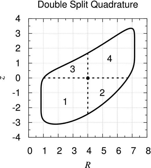
Sketch of double-split quadrature. In the numerical integration of the gravitational potential of an axisymmetric object at its internal point, we divide the integration domain into four numbered regions radially and vertically separated at the point. Depicted is a case when the cylindrical coordinates of the internal point are R = 4 and z = 0, which is indicated by a bullet in the figure, for a finite object with a convex cross-section.
Using the extended method, we prepared Figs 6– 9 illustrating the contour map of the computed gravitational potential of the axisymmetric objects the volume mass density of which are already shown in Figs 2–4. Because the mass density profile is convolved with a kernel function with a sharp peak and wide skirts, the resulting distribution of the gravitational potential resembles that of the density profile faithfully after slight rounding.
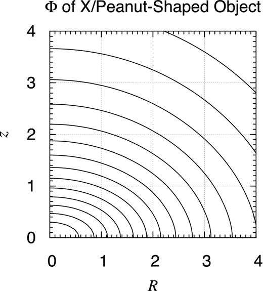
Potential contour map of X/peanut-shaped object. Shown is the contour map of the gravitational potential of the object the volume mass density of which is described in Fig. 2. The contours are drawn at every 5 per cent level of the bottom value, which is achieved at the coordinate centre. Omitted is the lower half part where z < 0 since the object is of the x–y plane symmetry. Despite the peculiar feature of the density contours shown in Fig. 2, the potential contours illustrated here are almost elliptical although they are not genuine ellipses.
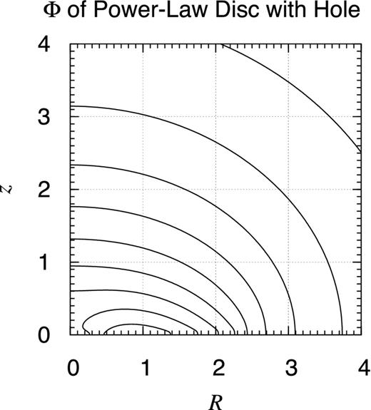
Potential contour map of power-law disc with hole. Same as Fig. 6 but for the power-law disc the density of which is depicted in Fig. 3. This time, the bottom value is achieved when R ≈ 0.85 and z = 0. If the spherically symmetric potential of a point mass of certain magnitude is superposed, it would result in a realistic model of the gravitational potential of TW Hya.
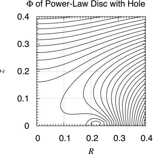
Potential contour map of power-law disc with hole: close-up. Same as Fig. 7 but focused is the central part. Notice that the disc exists in a limited region, R ≥ 0.2.

In this paper, we will describe the extended method in Section 2, examine its accuracy in Section 3, and provide some examples in Section 4.
2 METHOD
2.1 Integral expression of gravitational potential of axisymmetric object
Consider a general axisymmetric object of an infinite or finite size. Adopt the cylindrical coordinate system, (R, z). Denote the inner and outer radii of the object by Rin(≥ 0) and Rout(≤ +∞), respectively. Without losing the generality, we can assume that the volume mass density of the object, ρ(R, z), vanishes when z ≤ zlower(R) or z ≥ zupper(R), where zlower(R)(≥ −∞) and zupper(R)(≤ +∞) are certain functions of R as shown in Fig. 5. In fact, if the vertical boundary of the object is not uniquely described by functions of R, one may vertically split the object into several pieces so as to satisfy the condition.
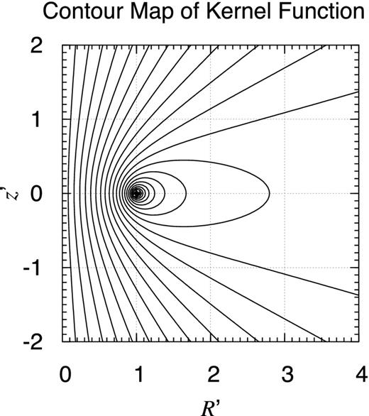
Contour map of kernel function. Illustrated is the contour map of the kernel function of the axisymmetric integral expression of the gravitational potential, g(R′, z′; R, z), when R = 1 and z = 0. The function has a blow-up logarithmic singularity at R′ = R and z′ = z, which is indicated by dense concentric circles around it.
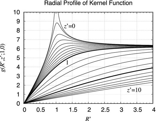
Radial profile of kernel function. Same as Fig. 10 but plotted as functions of R′ for various values of z′ as z′ = 0, 0.1, 0.2, 0.3, 0.4, 0.5, 0.6, 0.7, 0.8, 0.9, 1, 1.5, 2, 3, 4, 5, 6, 7, 8, 9, and 10. The thick curves are those for z′ = 1 and 5. The curve of z′ = 0 blows up logarithmically at R′ = 1.
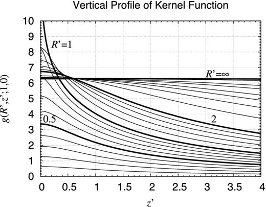
Vertical profile of kernel function. Same as Fig. 10 but plotted as functions of z′ for various values of R′ as R′ = 0.1, 0.2, 0.3, 0.4, 0.5, 0.6, 0.7, 0.8, 0.9, 1, 1.2, 1.4, 1.6, 1.8, 2, 3, 4, 5, 6, 8, 10, 20, and R′ → ∞. The thick curves show the cases when R′ = 0.5, 1, 2, and R′ → ∞. The curve of R′ = 1 blows up logarithmically at z′ = 0. The curve of R′ → ∞ is a constant value of 2π.
2.2 Piecewise density function
2.3 Vertical split quadrature
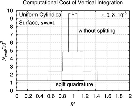
Computational cost of vertical integration. Shown is Neval, the number of function calls required in the numerical integration. Plotted are the results for a line integral representing the gravitational potential of an infinitely thin uniform cylindrical surface of the radius and the half height, a = c = 1. Compared are Neval as functions of R′, the radius of the location of the vertical line integral, of two methods using the DE quadrature rule with the relative error tolerance δ = 10−8: (i) the single quadrature without interval splitting, and (ii) the sum of two quadratures for the intervals split at z′ = z. The former method could not obtain the correct integral value when R′ ≈ a.
2.4 Radial split quadrature
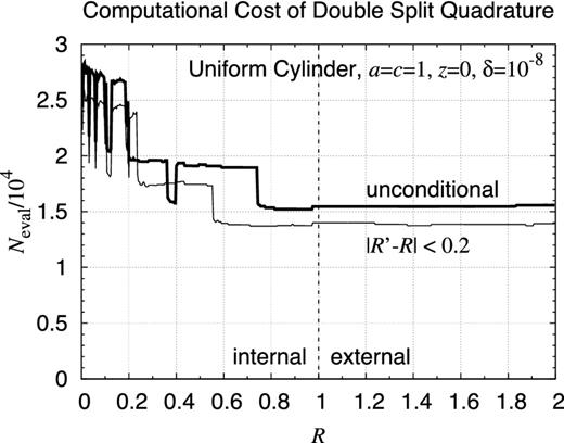
Computational cost of double-split quadrature. Same as Fig. 13 but for the numerical evaluation of a double integral representing the gravitational potential of a finite uniform cylinder of the radius and the half height as a = c = 1. Compared are two double-split quadrature methods using the DE rules: (i) that of unconditional radial splitting at R′ = R, and (ii) that with the radial splitting only when |R′ − R| < 0.2.
2.5 Parallel computing of split quadrature
The computational amount of the numerical integration by the DE rules is almost independent of the length of the interval. This is because the DE rules (i) transform the given integration interval, whether being infinite or finite, into an infinite interval, (−∞, +∞), and then (ii) compute the truncated trapezoidal sum (Press et al. 2007, section 4.5). If both the vertical and radial splitting is conducted, the gravitational potential computation is reduced to those of at least four integrals. Refer to Fig. 5 once again.
Each of the split integrals can be computed independently with each other and their computational times are roughly the same. Thus, appropriate is their parallel execution. Since the number of parallel computable pieces is as small as 2 typically and 6 or 8 at most, even an ordinary PC with 2–8 cores can be used for their parallel computation, say by employing the OpenMP architecture (OpenMP 2015).
2.6 Computation of acceleration vector
In principle, these differentiations are not well defined at some points where the potential is not analytic. Examples are some exponential disc models of spiral galaxies on the x–y plane and/or along the z-axis. However, the non-analyticity is an unphysical situation for a natural smoothly continuous body. Also, we may assign zero values in those cases if the object is of a certain symmetry such as those with respect to the x–y plane in almost all cases.
2.7 Calculation of circular speed
2.8 Implementation notes
As the programs of numerical quadrature, we recommend Ooura's efficient implementations of the DE rules, intde and intdei, the programs to obtain the integrals over a finite interval, (t1, t2), and over a semi-infinite interval, (t, ∞), respectively (Ooura 2006). In evaluating the double integrals, we prepare two sets of their copies, say intdez and intdeiz for the vertical integration and intder and intdeir for the radial integration. On the other hand, in computing the partial derivatives, we utilize dfridr, the fortran function listed in Press et al. (1992, section 5.7). Refer to Appendix B for the implementation notes on the parallel integration.
In computer programming, the usage of global variables is strongly discouraged (Brooks 1997). Here a variable is global when it is viewable from and rewritable by any subprogram. Its typical example is a variable in the common blocks of fortran. Global variables are disliked because, in general, (i) they make the interaction among subprograms so complicated, and as a result, (ii) they tend to generate erroneous computer codes. However, they are necessary in utilizing the ready-made programs like intde. This is because it would be cumbersome to specify all the variables/parameters explicitly as the arguments of the subprograms. In place of giving a general discussion, we present below the main part of a sample fortran code to evaluate the double integral, Φ(R, z), without the integration interval splitting:
real*8 function phiint(r,z)
...
common /param/rin,rout,zlower,zupper,rx,zx,rpx
rx=r; zx=z
call intder(psiint,rin,rout,eps,phiint,err)
return; end
real*8 function psiint(rp)
...
common /param/rin,rout,zlower,zupper,rx,zx,rpx
rpx=rp
call intdez(fint,zlower,zupper,eps,psiint,err)
return; end
real*8 function fint(zp)
...
common /param/rin,rout,zlower,zupper,rx,zx,rpx
fint=-rho(rpx,zp)*green(rpx,zp,rx,zx)
return; end
where |${\tt rx} = R$|, |${\tt zx} = z$|, and |${\tt rpx} = R^{\prime }$| are stored in a named common block and their numerical values are secretly passed by way of the block.
2.9 CPU time
One may think that the new method is time-consuming. This is only partially true. Table 1 lists the averaged CPU time of a single point evaluation of the gravitational potential of various infinitely extended objects, which will be explained later in Section 4 and Appendix E, by the new method when the relative error tolerance is set as moderate as δ = 10−8. The CPU times range 0.4–2.3 ms at an ordinary PC. On the other hand, Ridder's method requires 2–10 evaluations of the gravitational potential in general (Fukushima 2016). This amount is so small that the rotation curve of such an object is typically prepared in less than a second.
Averaged CPU time of potential computation. Shown are the averaged CPU times to compute a single point value of the gravitational potential by the new method when the relative error tolerance is set as moderate as δ = 10−8. The unit of the CPU time is ms at a PC with an Intel Core i7-4600U CPU running at 2.10 GHz clock while no parallel computing is employed. The results for various infinitely extended objects, the explanation of which are found in Section 4 and Appendix E, are listed in the increasing order of the CPU time.
| Object | CPU time (ms) |
|---|---|
| Gaussian spheroid | 0.41 |
| Perfect spheroid | 0.46 |
| Burkert spheroid | 0.46 |
| Modified Hubble spheroid | 0.47 |
| Plummer spheroid | 0.49 |
| Exponential/Gaussian object | 0.53 |
| Bi-exponential object | 0.55 |
| Navarro–Frenk–White spheroid | 0.60 |
| Exponential spheroid | 0.61 |
| Exponential/sech2 object | 0.63 |
| Flared bi-exponential object | 0.65 |
| Modified exponential spheroid | 0.71 |
| Hernquist spheroid | 0.71 |
| Differenced modified-exponential object | 0.71 |
| Boxy object | 0.74 |
| Einasto spheroid (i = 2) | 0.93 |
| Jaffe spheroid | 0.96 |
| Einasto spheroid (i = 4) | 0.98 |
| Differenced Gaussian spheroid | 1.23 |
| Einasto spheroid (i = 7) | 1.29 |
| Gaussian oval toroid | 1.57 |
| Sérsic spheroid (n = 2) | 1.87 |
| de Vaucouleurs spheroid | 2.23 |
| Sérsic spheroid (n = 1) | 2.28 |
| X/peanut-shaped object | 2.29 |
3 VALIDATION
3.1 Finite uniform spheroid
3.2 Miyamoto–Nagai model
3.3 Care for numerical differentiation
3.4 Computational errors
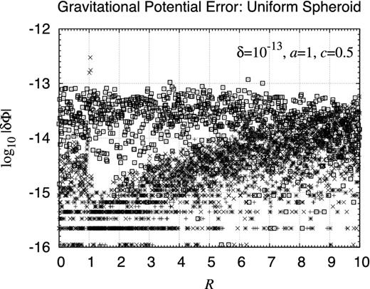
Integration error of gravitational potential: finite uniform spheroid. Shown are the integration errors of the gravitational potential of finite uniform spheroid obtained by the new method. Results are expressed as the base 10 logarithm of the normalized absolute errors of the potential numerically integrated with the relative error tolerance δ = 10−13. They are plotted as functions of R for several values of z as z = 0, 0.1, 1, and 10 while the semi-axes are fixed as a = 1 and c = 1/2. The errors of different z are overlapped since their distribution is almost the same.

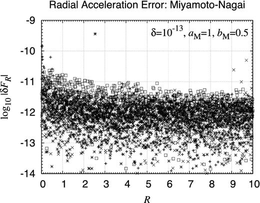
Computational error of acceleration vector of Miyamoto–Nagai model: radial component. Same as Fig. 16 but for the computational errors of the radial component acceleration.

Computational error of acceleration vector of Miyamoto–Nagai model: vertical component. Same as Fig. 17 but for the vertical component acceleration.
4 EXAMPLES
In order to show the performance of the new method, we present below the potential contour map and the rotation curve of a variety of axisymmetric objects. In Section 1, we already illustrated the contour map of the gravitational potential for fairly complicated objects: (i) an infinitely extended X/peanut-shaped object, (ii) a radially finite and vertically infinite power-law disc with a central hole, and (iii) an almost bounded tear-drop-shaped toroid with a non-analytic cross-section. On the other hand, the gravitational field of some simple axisymmetric objects is given in Appendices D and E. The former deals with some finite uniform objects, which are interesting from a theoretical view point, while the latter listed a number of infinitely extended spheroids, which will be useful in considering the gravitational field of the elliptical galaxies, the core/bulge of disc/spiral galaxies, and the visible and dark matter haloes.
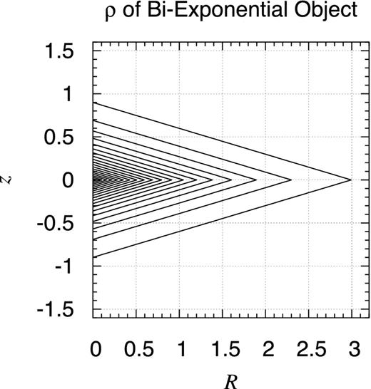
Density contour map of bi-exponential object. Shown is the contour map of the volume mass density of an axisymmetric object expressed as ρBE(R, z) ≡ ρ0 exp (−R/a − |z|/c) when the scalelength parameters are chosen as a = 1 and c = 0.3. The contours are drawn at every 5 per cent level of the peak value. They are rhombi of the aspect ratio, a: c = 10 : 3. Although the contours seem to be localized in a diamond-shaped region as R + |z|/0.3 ≤ 3, the object is infinitely extended in reality.
![Density contour map of flared bi-exponential object. Same as Fig. 19 but for an axisymmetric object with the volume mass density profile expressed as ρFE(R, z) ≡ ρ0 exp [−R/a − (|z|/c)/f(R/a)], where f(ξ) is a function describing the normalized vertical scaleheight as f(ξ) = 1 + kξ while the parameters are chosen as a = k = 1 and c = 0.3.](https://oup.silverchair-cdn.com/oup/backfile/Content_public/Journal/mnras/462/2/10.1093_mnras_stw1765/2/m_stw1765fig20.jpeg?Expires=1750253680&Signature=Ab2lGFYvRCgAXm0IKo7l~vNgYc3q9EI3Zlbjm-3vJMZgH88ZlA14m78qk8z1U41bHhhyi2~JhY4VwcY76R1VjQQZ~G8gAtpmFWp-fbEIrVDwJaVLLWxmKhRl~c6YAZFcDwSlrZ5wgE0MPnLbkw3YUT6jW-TFzSZQkSo5sBDxm3iPBCwtlIgSmtEvJepdmBdso4dbBCM51hwCyj98ASvzA5WoTHHj0AnTBpffV4WouIjq5m0G8LQjlSQ7tggVgza9h1vnXqGpraJ0TQCya8YCXo1eMTK7cn2Vv~K-KzSWdOa2KphMvEHwmXON2iEvjhaP9JOmxlsO4ctQqKWI3vR1gA__&Key-Pair-Id=APKAIE5G5CRDK6RD3PGA)
Density contour map of flared bi-exponential object. Same as Fig. 19 but for an axisymmetric object with the volume mass density profile expressed as ρFE(R, z) ≡ ρ0 exp [−R/a − (|z|/c)/f(R/a)], where f(ξ) is a function describing the normalized vertical scaleheight as f(ξ) = 1 + kξ while the parameters are chosen as a = k = 1 and c = 0.3.
![Density contour map of radially exponential and vertically secant-hyperbolic-squared disc. Same as Fig. 19 but when the volume mass density profile is expressed as ρES(R, z) ≡ ρ0 exp (−R/a) sech2[−|z|/(2c)], where a = 1 and c = 0.3.](https://oup.silverchair-cdn.com/oup/backfile/Content_public/Journal/mnras/462/2/10.1093_mnras_stw1765/2/m_stw1765fig21.jpeg?Expires=1750253680&Signature=Y8k5GPHj7Hb~gHoOCF70u~KoJb0TdDZt171efYDP-79iCTap5DkeITR1F7EOOP4crIGMx9KBJijnOujUYLJG0P7aRebn-cAMtr0UToBknDiYEYhK7fJo-bCXpc2926JIG17yAmQ9SIVXkP1j-fMJAFwrAB6Ig~09fxi7xeH7PtvNc~no4EzfLMaXyP9gtuX3-4tysWZTNWrMDn91j-Lwm2LlKgstKOsbnl4DklqtK-KGxhdAoUI2TRvBbxHLQ6XkUBllZ0vkUF2HQyNpaqr-flEjUe0op49WZ17hN~SJNbFXrijp3G~ZwcqVFeYJBt58xK0KRznhsDZDjcmypTKF4w__&Key-Pair-Id=APKAIE5G5CRDK6RD3PGA)
Density contour map of radially exponential and vertically secant-hyperbolic-squared disc. Same as Fig. 19 but when the volume mass density profile is expressed as ρES(R, z) ≡ ρ0 exp (−R/a) sech2[−|z|/(2c)], where a = 1 and c = 0.3.

Density contour map of radially exponential and vertically Gaussian disc. Same as Fig. 19 but when the volume mass density profile is expressed as ρEG(R, z) ≡ ρ0 exp (−R/a − z2/c2), where a = 1 and c = 0.3.
![Density contour map of boxy object. Same as Fig. 19 but when the volume mass density profile is expressed as $\rho _{\rm BX} (R,z) \equiv \rho _0 \exp \left[ - \sqrt{(R/a)^4 + (z/c)^4} \right]$, where a = 1 and c = 0.3.](https://oup.silverchair-cdn.com/oup/backfile/Content_public/Journal/mnras/462/2/10.1093_mnras_stw1765/2/m_stw1765fig23.jpeg?Expires=1750253680&Signature=snvk5YHc5mwGnyEVMfNvY3go3ZsA72UHfJURj5D2EfUjReCbZNT5wl4hjppbd8RraLBWgaBW3x0agLL~S6e~YVZvYgpRSdIeLM5qqs7qPtfrzTGD3PLYgk~Kmu-Nbbt51y6TH7jbZo1RGRfbbEcRdmvb9PRW-0A23SR4KinQy23ohnd5V4jg9r8l0z-YFGD7VmoKt5LC3ilLbb1TjHAUD~e0iBb0zxIZKwxhbo8JNg44g-gG0Yf-79Lfd-8vshTmpIunYJ6V74HcLZcftV4-UksWkE8JOegDSl5qCNh8JdqqXULuy1LX2lfnMNAOMiBCunSOPBqc9AWdtf15Gzec3g__&Key-Pair-Id=APKAIE5G5CRDK6RD3PGA)
Density contour map of boxy object. Same as Fig. 19 but when the volume mass density profile is expressed as |$\rho _{\rm BX} (R,z) \equiv \rho _0 \exp \left[ - \sqrt{(R/a)^4 + (z/c)^4} \right]$|, where a = 1 and c = 0.3.
![Density profile of Gaussian oval toroid. Same as Fig. E2 but for a toroid with the volume mass density written as ρGT(R, z) ≡ ρ0 exp [−{(R − RT)/a}2 − {(|z|/c)/f(R/a)}2], where f(ξ) ≡ 1 + kξ is a linear flaring function while the parameters are set as RT = 2, a = 1, c = 0.3, and k = 0.7. We determined the functional form and the parameters to mimic the result of N-body simulation of particle swarm with a toroidal feature (Bannikova, Vakulik & Sergeev 2012, fig. 10).](https://oup.silverchair-cdn.com/oup/backfile/Content_public/Journal/mnras/462/2/10.1093_mnras_stw1765/2/m_stw1765fig24.jpeg?Expires=1750253680&Signature=NC~ZqmVv2JC~hZRlXCUGATVf3fkqLtJ3VsO9sST51Dvl8tl7vVJFcJ19AMCPScTadNP147dLzHHL~DmNJ3ncNHbYtH57SU857cQ1NGImaJAKaRNaEXaTChgHIY~ZYRtybofSlLtWlKOMJqMc7nIGGZSuB7-ifeIRosth~XH4nOisu-gNGkiu5bFgF8YJfoxS1xZVrif8MpwYAD2J~aSvjwjGDEgXzyAUNQInsiK8HXgqKNTDESl2bGO9zpBxqHz2~MT1yjvwB~eWXqtE9UoLWJTD5TZ~ftZqdM5uaHHOGwg68qooddgxcwYEXnj~JcVYYaM5AGTN4vmnwxMC4j9KAQ__&Key-Pair-Id=APKAIE5G5CRDK6RD3PGA)
Density profile of Gaussian oval toroid. Same as Fig. E2 but for a toroid with the volume mass density written as ρGT(R, z) ≡ ρ0 exp [−{(R − RT)/a}2 − {(|z|/c)/f(R/a)}2], where f(ξ) ≡ 1 + kξ is a linear flaring function while the parameters are set as RT = 2, a = 1, c = 0.3, and k = 0.7. We determined the functional form and the parameters to mimic the result of N-body simulation of particle swarm with a toroidal feature (Bannikova, Vakulik & Sergeev 2012, fig. 10).
Let us explain the background of these objects one by one. First, a bi-exponential disc is a simple but realistic model of the thick stellar disc and/or of the interstellar medium (ISM), namely the gas and dust, of the spiral galaxies (Bahcall & Soneira 1980). In fact, Fig. 19, namely the case when c/a = 0.3, approximates the thick stellar disc of the Milky Way if the unit distance is chosen as 4.0 kpc (Robin et al. 2012, table 2). Also, the bi-exponential disc when c/a = 0.03 resembles the ISM of the Milky Way if the unit distance is chosen as 4.5 kpc (Robin et al. 2003, table 3). Of course, the infinitely thin limit when c → 0 is nothing but the infinitely thin exponential disc (Freeman 1970).
Secondly, the gas discs of many edge-on galaxies show a flaring (van der Kruit 2008). Although some profiles indicate a more rapid increase (O'Brien et al. 2010a; O'Brien, Freeman & van der Kruit 2010b,c,d), we assume here a linear flaring as ρFE(R, z) for simplicity.
Thirdly, there exist a few variations on the vertical profile of a bi-exponential disc: the Gaussian decay, the exponential damping, and their linear combination. A recent investigation (Robin et al. 2014) implies that the vertical profile of the thick stellar disc component of the Milky Way seems to be in proportion to the square of the secant hyperbolic function as ρES(R, z).
Fourthly, some galaxies including LEDA 074886 exhibit a boxy outlook like ρBX(R, z) (Graham et al. 2012).
Fifthly, practically important is the difference of representative spheroidal distributions like (i) the differenced Gaussian spheroid as ρDG(R, z), and (ii) the differenced modified exponential spheroid as ρDM(R, z). For example, in the Besançon Galaxy model, the thin discs of young and old stars are approximated by the former and the latter, respectively (Robin et al. 2003). In principle, their gravitational field can be obtained as the difference of the gravitational field of the undifferenced spheroids as shown in Appendix E. However, since the structure is so different, we shall discuss them here as special examples.
Finally, as a simple model of toroidal object, we consider a Gaussian toroid with a flared scaleheight. Its functional form was hinted from the result of N-body simulation of a particle swarm (Bannikova et al. 2012).
Using the new method, we evaluated the gravitational potential of these objects. Refer to Figs 25– 37 for the contour map of the gravitational potential of these objects when a = 1, c = 0.3, and the other parameters are appropriately specified. Also, we prepared the associated rotation curves of these objects for various values of the aspect ratio, c/a, in Figs 38–46. Refer to Fig. 47 for the comparison of the rotation curves of some selected objects for the same aspect ratio, c/a = 0.3.
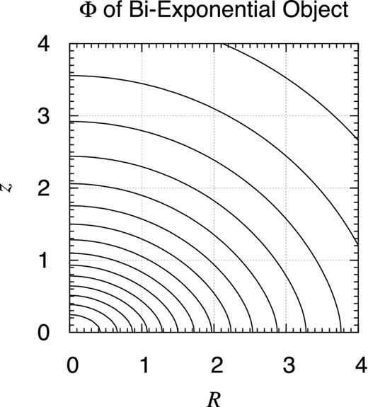
Potential contour map of bi-exponential object. Same as Fig. 6 but for the bi-exponential object. Its volume mass density is described as ρBE(R, z) ≡ ρ0 exp (−R/a − |z|/c) when a = 1 and c = 0.3. This distribution resembles that of the thick stellar disc of the Milky Way if the unit distance is chosen as 4.0 kpc (Robin et al. 2003, table 3). The contours are drawn at every 5 per cent level of the bottom value. The potential is not analytic on the x–y plane and along the z-axis, although the non-analyticity is hardly visible at this scale.
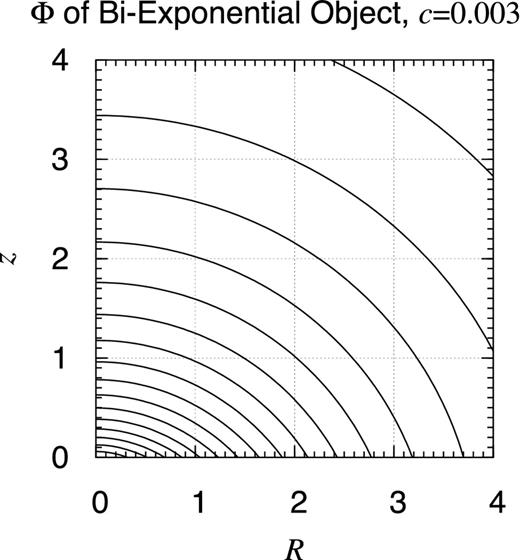
Potential contour map of bi-exponential object: c = 0.003. Same as Fig. 25 but when c = 0.003. At this scale, observed will be no further difference in the potential contour map when c ≤ 0.003. In this sense, the contour map shown here is practically the same as that of the infinitely thin exponential disc (Freeman 1970). This time, the non-analyticity on the x–y plane is obvious.
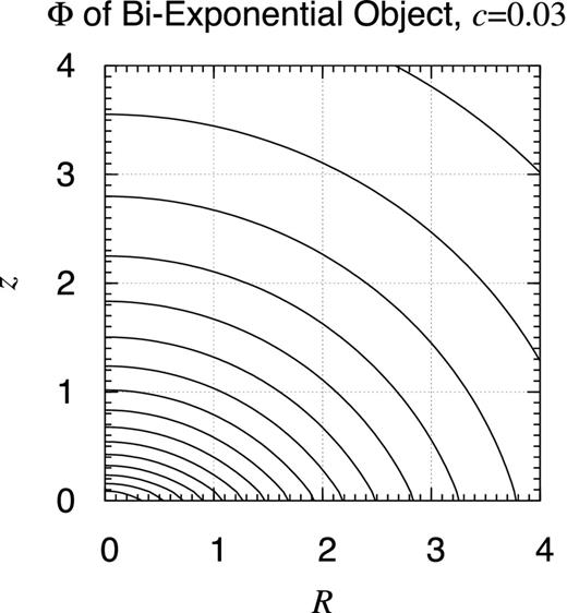
Potential contour map of bi-exponential object: c = 0.03. Same as Fig. 25 but when c = 0.03. This approximates the contour map of the gravitational potential of the ISM disc of the Milky Way if the unit distance is chosen as 4.5 kpc (Robin et al. 2003, table 3). Still visible is the non-analyticity on the x–y plane.
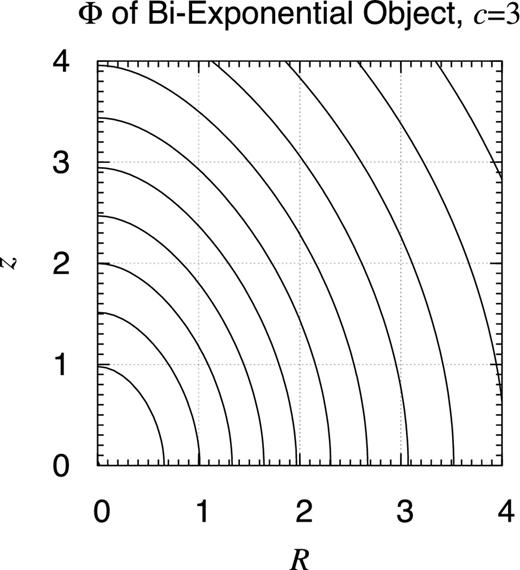
Potential contour map of bi-exponential object: c = 3. Same as Fig. 25 but when c = 3.
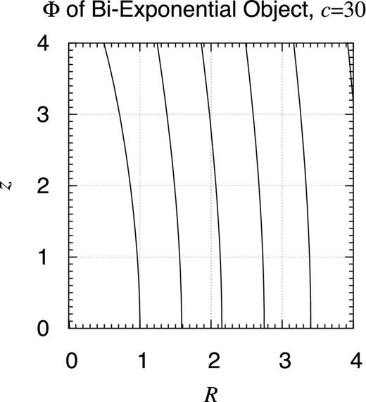
Potential contour map of bi-exponential object: c = 30. Same as Fig. 25 but when c = 30.
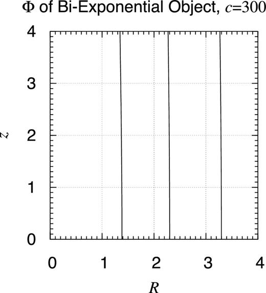
Potential contour map of bi-exponential object: c = 300. Same as Fig. 25 but when c = 300. At this scale, observed will be no further difference in the potential contour map when c ≥ 300.
![Potential contour map of flared bi-exponential object. Same as Fig. 25 but for a flared bi-exponential object. Its volume mass density is described as ρFE(R, z) ≡ ρ0 exp [−R/a − (|z|/c)/f(R/a)], where f(ξ) = 1 + kξ. Shown is the result when a = k = 1 and c = 0.3.](https://oup.silverchair-cdn.com/oup/backfile/Content_public/Journal/mnras/462/2/10.1093_mnras_stw1765/2/m_stw1765fig31.jpeg?Expires=1750253680&Signature=3qBQodMdiq8cHFmdBBE14VffI~mbRnk61I4A7MM6YTOk0571wTPNB0uCUu7F4j4CT23xNgzkJaCfuxCNzEktgp3zzNDH~fFC2JSl5VjJOemHPx2AAnh-BeVWJFCDa6fJWDBlR6IYTbpE6YZ8tmK3gyrVIBMyXEgCeqAj6-rcLy5G2o42Zbh16HIKOGvcfuXbCl4ESVLonudAd2jcnoTCH4bFIug-y54OXs8gRJkTE-FWHSTW49UBb2H3vqtxZhvVgbnwBLULUmh~d836YM73COLnQRDWluOTKKCt~PDguD6QNNAB1jDnagTVbQjlB0V7G5C6XxLLXtkq6lMFMtjdGA__&Key-Pair-Id=APKAIE5G5CRDK6RD3PGA)
Potential contour map of flared bi-exponential object. Same as Fig. 25 but for a flared bi-exponential object. Its volume mass density is described as ρFE(R, z) ≡ ρ0 exp [−R/a − (|z|/c)/f(R/a)], where f(ξ) = 1 + kξ. Shown is the result when a = k = 1 and c = 0.3.
![Potential contour map of radially exponential and vertically secant-hyperbolic-squared object. Same as Fig. 25 but when the volume mass density profile is given as ρES(R, z) ≡ ρ0 exp (−R/a) sech2[−|z|/(2c)] when a = 1 and c = 0.3.](https://oup.silverchair-cdn.com/oup/backfile/Content_public/Journal/mnras/462/2/10.1093_mnras_stw1765/2/m_stw1765fig32.jpeg?Expires=1750253680&Signature=iKHn~JdRYajjQ9p4ruvMmW3BMCJ~XQyyBj4SCAG6IliObRGFvt46MU~2x1EBsQqP3cj8qjOp0LBMM-p6jLVPz1kJ833l-jKGJLYAL5GDHX6Yl6ghB7~bB7gVBQNzOpY0Ht1xRPCB4~KtSwUEZJKIIuSMzUD~yx~Y7uB1vPtEx1lqSgkteYu-05YGvgmyT68d7iMSlzR8KgWJW7QTSql0n4z6UYyC53W84-gDr6u1-BAfockfoFhjrY8LLHtbjFaH6FMMZsNr7dDid9x2C54OZNMSVdKFfOejqqW8nBwxi2ivDlBKxcOs2BjTCFocm776DcYD5mm50jLSREz8Krd7GA__&Key-Pair-Id=APKAIE5G5CRDK6RD3PGA)
Potential contour map of radially exponential and vertically secant-hyperbolic-squared object. Same as Fig. 25 but when the volume mass density profile is given as ρES(R, z) ≡ ρ0 exp (−R/a) sech2[−|z|/(2c)] when a = 1 and c = 0.3.
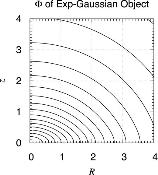
Potential contour map of radially exponential and vertically Gaussian object. Same as Fig. 25 but when the volume mass density profile is given as ρEG(R, z) ≡ ρ0 exp (−R/a − z2/c2) when a = 1 and c = 0.3.
![Potential contour map of boxy object. Same as Fig. 25 but when the volume mass density profile is expressed as $\rho _{\rm BX} (R,z) \equiv \rho _0 \exp \left[ - \sqrt{(R/a)^4 + (z/c)^4} \right]$ when a = 1 and c = 0.3.](https://oup.silverchair-cdn.com/oup/backfile/Content_public/Journal/mnras/462/2/10.1093_mnras_stw1765/2/m_stw1765fig34.jpeg?Expires=1750253680&Signature=poSic-Q9saNfr6MBJ6Wfnn5ZVNFqJWfF2L~0qNtCoRsY6K1lsDDBakdtXyzJ0mxXAUWyNKnzRUNckDjVtrWmn2T7qpS3TUs4RKAqEBFMav-Ngudlwp~9sipZM2WYElph6udrht3ye5AURifEpbl53pFgENYCvVS-APS9eB-J-wWTlZWLiQqD~gSXRewB5Fopp6xJAiQFBoH2fLPPAfveZyDdia5KCW31dRP1rcvW2VnON5uoNZZBieeJS2S0fGd67EdSbmsVpmoK1BhgaBs3C4j4hUHVhCoyIAVyGBA6Kww3rwFfWxGaciB~895z0ZTBBnol-7h9SZkhRUQDj3W4nA__&Key-Pair-Id=APKAIE5G5CRDK6RD3PGA)
Potential contour map of boxy object. Same as Fig. 25 but when the volume mass density profile is expressed as |$\rho _{\rm BX} (R,z) \equiv \rho _0 \exp \left[ - \sqrt{(R/a)^4 + (z/c)^4} \right]$| when a = 1 and c = 0.3.
![Potential contour map of differenced Gaussian spheroid. Same as Fig. 25 but when the volume mass density profile is given as $\rho _{\rm DG} (R,z) \equiv \rho _0 \left[ \exp \left( - s_{\rm out}^2 \right) - \exp \left( - s_{\rm in}^2 \right) \right]$, where $s_{\rm out} \equiv \sqrt{R^2/a_{\rm out}^2 + z^2/c_{\rm out}^2}$, $s_{\rm in} \equiv \sqrt{R^2/a_{\rm in}^2 + z^2/c_{\rm in}^2}$, while aout = 2, cout = 0.6, ain = 1, and cin = 0.3. Notice that the central concentration is significantly reduced.](https://oup.silverchair-cdn.com/oup/backfile/Content_public/Journal/mnras/462/2/10.1093_mnras_stw1765/2/m_stw1765fig35.jpeg?Expires=1750253680&Signature=2VhPIAV3O9PchrZz9s3kRxB7IyqdRvR2ABrN7ZMnKqV-AMTHOYiXkX8lUczSqhuGSecwT-qT3uYkRZ96x5wgJb9w5HqMF0xAMMYVX3LPey8swYH0YSf2Bpy6Rz12UTprISjmuQ~dHl5k~~pUe1hJFS7d0yUvvHNTYjq-CImRVWaFIOeZtpxspdxTaiWAE9Qxn75bunvTgIT7q4jZwwZK~PwqMyIrXIVRyhxyeFrWn~AbknXbYpi2nxe-rSDDQ1GW2Xf-9Q2TD9jp5sKmvPc6--rO-NDnRjP~XtfsclmSU9D4C8K01-K8s7h25LXVc87YTUlC192b8GqVE~IODZg7vQ__&Key-Pair-Id=APKAIE5G5CRDK6RD3PGA)
Potential contour map of differenced Gaussian spheroid. Same as Fig. 25 but when the volume mass density profile is given as |$\rho _{\rm DG} (R,z) \equiv \rho _0 \left[ \exp \left( - s_{\rm out}^2 \right) - \exp \left( - s_{\rm in}^2 \right) \right]$|, where |$s_{\rm out} \equiv \sqrt{R^2/a_{\rm out}^2 + z^2/c_{\rm out}^2}$|, |$s_{\rm in} \equiv \sqrt{R^2/a_{\rm in}^2 + z^2/c_{\rm in}^2}$|, while aout = 2, cout = 0.6, ain = 1, and cin = 0.3. Notice that the central concentration is significantly reduced.
![Potential contour map of differenced modified exponential spheroid. Same as Fig. 35 but when the volume mass density profile is given as ρDM(R, z) ≡ ρ0[exp (−σout) − exp (−σin)], where $\sigma _{\rm out} \equiv 2s_{\rm out}^2/ (1 + \sqrt{1+4s_{\rm out}^2})$, $\sigma _{\rm in} \equiv 2s_{\rm in}^2/ (1 + \sqrt{1+4s_{\rm in}^2} )$, while $s_{\rm out} \equiv \sqrt{R^2/a_{\rm out}^2 + z^2/c_{\rm out}^2}$, $s_{\rm in} \equiv \sqrt{R^2/a_{\rm in}^2 + z^2/c_{\rm in}^2}$, and aout = 2, cout = 0.6, ain = 1, and cin = 0.3. The central concentration is further reduced.](https://oup.silverchair-cdn.com/oup/backfile/Content_public/Journal/mnras/462/2/10.1093_mnras_stw1765/2/m_stw1765fig36.jpeg?Expires=1750253680&Signature=kBBSkFmLVHNsTi35HQsHExu9EgtTcLA~A25qnNgUxfwrbLa2OkrtTvvi07mVWWEL4l08ex~p7MoQvHKrLpx9z4pWjWuasrntI58JmuultJH2Psl-Krxq5wiQ847pluS4svnXcH6EC~047TIZzDAT6~78-0TPzpPQwZoHZi3d9htm1VAAyOIMx6nKWDl4IwDX27Jh6WTvNb7hcrJuAmvltJM~fDg470f2KTYz8mbk0YjJoYyb2HNW~8BEp3igJ1opMzktuiRwxA7ETFoAmUG7c8bsjuCfMwMPO2CRWcR70N2zWDdas8-FwtQi~m2qdx8ZmZBuYlcnG7v82~b3sb625A__&Key-Pair-Id=APKAIE5G5CRDK6RD3PGA)
Potential contour map of differenced modified exponential spheroid. Same as Fig. 35 but when the volume mass density profile is given as ρDM(R, z) ≡ ρ0[exp (−σout) − exp (−σin)], where |$\sigma _{\rm out} \equiv 2s_{\rm out}^2/ (1 + \sqrt{1+4s_{\rm out}^2})$|, |$\sigma _{\rm in} \equiv 2s_{\rm in}^2/ (1 + \sqrt{1+4s_{\rm in}^2} )$|, while |$s_{\rm out} \equiv \sqrt{R^2/a_{\rm out}^2 + z^2/c_{\rm out}^2}$|, |$s_{\rm in} \equiv \sqrt{R^2/a_{\rm in}^2 + z^2/c_{\rm in}^2}$|, and aout = 2, cout = 0.6, ain = 1, and cin = 0.3. The central concentration is further reduced.
Examine these results one by one. First, Fig. 25 illustrates that, despite the rhombic feature of the density contours shown in Fig. 19, the potential contours depicted here are almost elliptical. Of course, the contours are not genuine ellipses. In fact, they are not analytical along the z-axis and on the x–y plane although the non-analyticity is hardly visible at this scale. At any rate, impressive is a significant difference in the potential and density contour maps.
Let us investigate the details of the bi-exponential objects, especially the effect of the aspect ratio. Figs 26– 30 show the similar potential contour map for several values of c as c = 0.003, 0.03, 3, 30, and 300 while a is fixed as a = 1. That of the case when c = 0.3 is already shown in Fig. 25. As noticed already, the case when c/a = 0.03 well represents the gravitational potential of the ISM disc of the Milky Way if a is chosen as 4.5 kpc (Robin et al. 2003, table 3). Also, when c/a is sufficiently small, say when c/a ≤ 0.003, no qualitative difference is observed from the infinitely thin limit, namely the infinitely thin exponential disc (Freeman 1970).
Another point of interest is the effect of flaring. Fig. 31 shows the contour map of the gravitational potential of the flared bi-exponential disc when a = 1 and c = 0.3. Its comparison with the unflared case, Fig. 25, may give an impression that the effect of flaring is small. In order to investigate its details, we prepared Fig. 40 showing the rotation curves for various values of the flaring factor, k, as k = 0 through k = 5. The comparison of the rotation curves reveals that, when k increases, the peak location moves outwards, although the outlook of the rotation curves is almost the same.
The volume mass density distribution of thin discs in the vertical direction is a controversial issue. One possibility is the same exponential damping as described by the bi-exponential objects. However, this vertical profile has a kink on the x–y plane. As a result, the resulting gravitational potential is continuous but non-analytic on the plane. This is unphysical.
Other options to conquer this problem are the vertical distribution described by (i) the squared secant hyperbolic function as ρES(R, z) described in equation (46), and (ii) the Gaussian distribution as ρEG(R, z) described in equation (47). Indeed, Figs 32 and 33 provide the smoother contour maps of their gravitational potential, although the flattening of the contours are different.
Meanwhile, the bulge components of some disc/spiral galaxies exhibit a boxy feature like that described in equation (48). In this specific case, Fig. 34 indicates that the central concentration is stronger despite the fact that the elliptical outlook of contours is almost unchanged.
In some models of the stellar mass distribution, the age difference is reflected to the difference of spatial distributions. For example, the Besançon Galaxy model adopted a classification of the thin stellar disc into seven components of different ages and assigned the differenced Gaussian or modified Gaussian spheroids to each of them (Robin et al. 2003, table 3). Figs 35 and 36 present the potential contour map of these difference spheroids. Obvious is the central flatness of the potential values. This is well reflected in their rotation curves depicted in Figs 44 and 45. These figures illustrate that the initial rise of the circular speed is not linear but quadratic with respect to R.
Finally, Fig. 37 shows the contour map of the gravitational potential of a toroidal object. Although Fig. 24 indicates the density distribution in a rather limited cross-section, the potential distribution extends to the whole space. For example, the coordinate origin is a saddle point and the minimum potential value is achieved at a circular ring where R ≈ 1.6 and z = 0. As a result, Fig. 46 shows that the inner part of the rotation curve is not properly defined. This never means an unphysical situation. Refer to Appendix D for the similar phenomena in some uniform objects illustrated in Figs D14, D17, and D18.
![Potential contour map of Gaussian oval toroid. Same as Fig. 25 but when the volume mass density profile is given as ρGT(R, z) ≡ ρ0 exp [−(R − RT)2/a2 − {(z/c)/f(R/a)}2] while a = 1, c = 0.3, RT = 2, and k = 0.7.](https://oup.silverchair-cdn.com/oup/backfile/Content_public/Journal/mnras/462/2/10.1093_mnras_stw1765/2/m_stw1765fig37.jpeg?Expires=1750253680&Signature=4MGX6mwbFV6sbP0a4KVXI6FZ3TSdlhUxJiUjqJWNtXh7a315Qh0y-UCi09VehtTbD0ToPLjvfWoLuUhxr6c9Q-HsjxTH4REZRF9U-6TbsxQFlVJYUY~W3OOB-8lzemxGFKZUmJWny3dCPg-GSq1YS2q4h7ccRfdxlqnG8ei095ffT6rCgqh1tX6wUyr76YIyFw~U~e2VKCaM4fg0e5xMuj0BcV6FjtupDK4rRRT-JXIkEhhQPbRWNLrLiBH8VXuL4hXE6kFW63R5blqPv061KaVLBZhLT42kCth7BD8Y-9dDNdeNcHH2z8XzcnqbyoJrZQeOPZWtHQHQvVAs~sNlSQ__&Key-Pair-Id=APKAIE5G5CRDK6RD3PGA)
Potential contour map of Gaussian oval toroid. Same as Fig. 25 but when the volume mass density profile is given as ρGT(R, z) ≡ ρ0 exp [−(R − RT)2/a2 − {(z/c)/f(R/a)}2] while a = 1, c = 0.3, RT = 2, and k = 0.7.
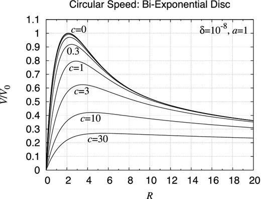
Rotation curve: bi-exponential object. Shown are the rotation curves of bi-exponential objects the volume mass density of which are expressed as ρBE(R, z) ≡ ρ0 exp (−R/a − |z|/c). Plotted are the circular velocities for various values of c as c = 0.001, 0.003, 0.01, 0.03, 0.1, 0.3, 1, 3, 10, and 30 while a is fixed as a = 1. The normalization constant V0 is arranged such that the total masses of the objects are the same. As a result, all the curves approach to the same functional form, namely that of a point mass, when R → ∞. At this scale, invisible is the departure of the curves when c ≤ 0.01 from the limit of c = 0, namely the rotation curve of the infinitely thin exponential disc described by a cross-product of the modified Bessel functions (Freeman 1970).
![Rotation curve: flared bi-exponential object. Same as Fig. 38 but for an object with the volume mass density expressed as ρFE(R, z) ≡ ρ0 exp [−(R/a) − (|z|/c)/f(R/a)], where f(ξ) ≡ 1 + kξ.](https://oup.silverchair-cdn.com/oup/backfile/Content_public/Journal/mnras/462/2/10.1093_mnras_stw1765/2/m_stw1765fig39.jpeg?Expires=1750253680&Signature=LF9iQjPZGXFMewE2qLEM3W-tAIAEQwD4roOSMmrh6tlXsyMvQey4Kz83GpNFC~4c-udbQAK~hvC9CwP9E6V~is7cpID9zMZPG2o9dOTpHl~vU1QWNBmyijKouosdvU76Ny3~wNqjRljK-z~35ri7XMKpKr7vHMcuLb4KV0qOULkGjBEzQZRTKVG3eJnvoG0zzwhnnh6YUxGxFyAb29slB9eLHQ1ULVDmWAmnPXE6fSxqvMGDkaS45fEazFgOlB4s0BMGYJ6Xqbl0qBKOoR0TlDOpKSvv60NEC8jDXIM55iiC2nJNrdpxUpBpxIJpjPOhG6i7Dncjv2iLsZdWTEU4wQ__&Key-Pair-Id=APKAIE5G5CRDK6RD3PGA)
Rotation curve: flared bi-exponential object. Same as Fig. 38 but for an object with the volume mass density expressed as ρFE(R, z) ≡ ρ0 exp [−(R/a) − (|z|/c)/f(R/a)], where f(ξ) ≡ 1 + kξ.
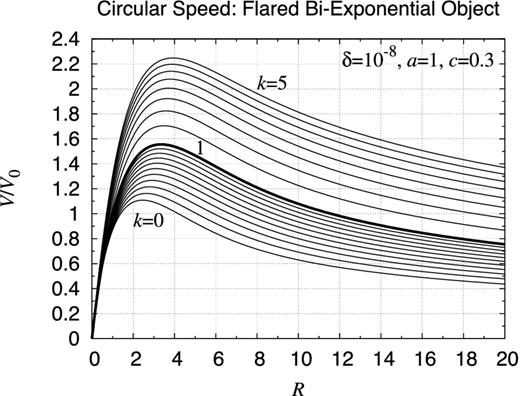
Rotation curve of flared bi-exponential object. Same as Fig. 39 but plotted are the curves for various values of k, the flaring factor, while the other parameters are fixed as a = 1, c = 0.3. Compared are the results for k = 0, 0.1, 0.2, 0.3, 0.4, 0.5, 0.6, 0.7, 0.8, 0.9, 1, 1.5, 2, 2.5, 3, 3.5, 4, 4.5, and 5. This time, the nominal density value ρ0 is set the same. The thick curve is the case of k = 1.
![Rotation curve: radially exponential and vertically secant-hyperbolic-squared object. Same as Fig. 38 but for an object with the volume mass density expressed as ρES(R, z) ≡ ρ0 exp (−R/a)sech2[|z|/(2c)].](https://oup.silverchair-cdn.com/oup/backfile/Content_public/Journal/mnras/462/2/10.1093_mnras_stw1765/2/m_stw1765fig41.jpeg?Expires=1750253680&Signature=VAuP53VKOAcDrF44AhsLAmcKUYeNXEZiLALbpn4sFTHAs7NZX7d7aT-6lNPvYLf9U0J0acr3RU14PcH6VJFTk~70yLUIDduqDykjTeqGaA-ZtyZ079VjjCc2N~m2qQ-GgV1b9p1UQK67Q03lfCvOZPw~jx7Hk8z1i~t4S~6g7hdCO0MBNMjVgbq~Afo3RCAXgwsAxbUup-J82yfKS9jgipBUvUJo7hIaFsVGXG8jXZtbC4h3IrGrWvCc3aNrwnL5giaoorrOxcwnAvg5hs-AOWU~irOSeIu5jyh-8PSxFkphEHIlCKT79GPT05AiW4cro0SIqw4jq-XV~FOU~EHdUA__&Key-Pair-Id=APKAIE5G5CRDK6RD3PGA)
Rotation curve: radially exponential and vertically secant-hyperbolic-squared object. Same as Fig. 38 but for an object with the volume mass density expressed as ρES(R, z) ≡ ρ0 exp (−R/a)sech2[|z|/(2c)].
![Rotation curve: radially exponential and vertically Gaussian object. Same as Fig. 38 but for an object with the volume mass density expressed as ρ(R, z) = ρ0 exp [−(R/a) − (z/c)2].](https://oup.silverchair-cdn.com/oup/backfile/Content_public/Journal/mnras/462/2/10.1093_mnras_stw1765/2/m_stw1765fig42.jpeg?Expires=1750253680&Signature=rDeIHgejtngQEmLBFX9DspdZljgg3mcvEzeBctK7VycFj9idX1d2VWhzdx6s9R3yuxCtqLSaoiDrzUSKcQ-6ccB4sqGficQQ6ow2oArLL~ccCr074aBMtaDyOM6c4BWxwEneY9vAIED8dQoUaKbY5r4ik9DS54anKwTVD5yu8ETLQlQrf9icAOWLg11g4askW2jmm-2Mh4Ejbs1UMWniI83zlbi7OpWclCs5rQg-iyDryOHXW9IuRxReKtVdrBRXUFNncs4s8ATh~CQUJQfisoGsZ1i4MoxJG~WJrC9u7sXUIl8DhdthonZ0XX3DtIa0qEVHNM~ZvHXh3HHJB27rcQ__&Key-Pair-Id=APKAIE5G5CRDK6RD3PGA)
Rotation curve: radially exponential and vertically Gaussian object. Same as Fig. 38 but for an object with the volume mass density expressed as ρ(R, z) = ρ0 exp [−(R/a) − (z/c)2].
![Rotation curve: radially exponential and vertically secant-hyperbolic-squared disc. Same as Fig. 38 but for an object with the volume mass density expressed as $\rho (R,z) = \rho _0 \exp [ - \sqrt{(R/a)^4+(z/c)^4}]$.](https://oup.silverchair-cdn.com/oup/backfile/Content_public/Journal/mnras/462/2/10.1093_mnras_stw1765/2/m_stw1765fig43.jpeg?Expires=1750253680&Signature=bo~BMyRapLo1xwVafdetq-w8wHZerR9Dv05Cq6pIHQanzK47w~M~9ZMW0anc0NUxzwH0G84wXaeRg9LiR9btzajz0akw9mvqLz11ulciJCZxPaFyagLSCvv6fpGQIGkghqLLJyil~zz90kYc-0rN0u6OOmEabIRL7W4c31wfZusrKnK-5TPmDlJfKkspZXC2GCWdEw12vlDWNs4ng21vBHccEUIVe8C70AAwmwFARaERt57uzDC6VcbPrjGU156juVghzCZulCnT-nxuQU6eQijOY5D5yhd6Ztq9h7Q2kYhsxNJmR1EVqbdCpcbYrK87G1gEY1RoGF6tMKLRA7GNDg__&Key-Pair-Id=APKAIE5G5CRDK6RD3PGA)
Rotation curve: radially exponential and vertically secant-hyperbolic-squared disc. Same as Fig. 38 but for an object with the volume mass density expressed as |$\rho (R,z) = \rho _0 \exp [ - \sqrt{(R/a)^4+(z/c)^4}]$|.
![Rotation curve: differenced Gaussian spheroid. Same as Fig. 38 but for an object with the volume mass density expressed as $\rho _{\Delta {\rm G}} (R,z) \equiv \rho _{\rm G}( s_{\rm out}) - \rho _{\rm G}( s_{\rm in}) = \rho _0[ \exp( - s_{\rm out}^2) - \exp( - s_{\rm in}^2)]$, where the auxiliary arguments are defined as $s_{\rm out} \equiv \sqrt{( R/a_{\rm out})^2 + ( z/c_{\rm out})^2}$ and $s_{\rm in} \equiv \sqrt{( R/a_{\rm in})^2 +( z/c_{\rm in})^2}$ while the constants are set as aout = 2a, cout = 2c, ain = a, and cin = c.](https://oup.silverchair-cdn.com/oup/backfile/Content_public/Journal/mnras/462/2/10.1093_mnras_stw1765/2/m_stw1765fig44.jpeg?Expires=1750253680&Signature=x7YS0pk~2zNR6HZO~ukRLAuP5sApw10HfCPR45W-6a-73oSl~KjF2Q5N4OAEPKYR3EDJT8-jQfzIFaxSjjcEBDEeZAQYhfznbOwNOwW2IB4YPbYjtp~N7YjdQ-UbIZ0MWF6DMPLKopT3uoRki78Za~g~hOBJKLzgGHcXxXqdgAADPzU6XlGjgdAXDc~cc5-zNhvz3DdObjY9R2L5RjbEPFquIu5CEZTw1MWn5qbaekkl-oeq~qHT9jM9FysM0B2YY5tKEzhf5R-R3WZcUK5j-dm9S5QNQnQyGAnA8Zcm0psFwWrRHlJ4VucUxpLSrjCV7vluVLtq6SFGgAO2~ATdYA__&Key-Pair-Id=APKAIE5G5CRDK6RD3PGA)
Rotation curve: differenced Gaussian spheroid. Same as Fig. 38 but for an object with the volume mass density expressed as |$\rho _{\Delta {\rm G}} (R,z) \equiv \rho _{\rm G}( s_{\rm out}) - \rho _{\rm G}( s_{\rm in}) = \rho _0[ \exp( - s_{\rm out}^2) - \exp( - s_{\rm in}^2)]$|, where the auxiliary arguments are defined as |$s_{\rm out} \equiv \sqrt{( R/a_{\rm out})^2 + ( z/c_{\rm out})^2}$| and |$s_{\rm in} \equiv \sqrt{( R/a_{\rm in})^2 +( z/c_{\rm in})^2}$| while the constants are set as aout = 2a, cout = 2c, ain = a, and cin = c.
![Rotation curve: differenced modified exponential spheroid. Same as Fig. 44 but for an object with the volume mass density expressed as $\rho _{\rm DM} (R,z) \equiv \rho _0 [ \exp\lbrace - 2 s_{\rm out}^2 / ( 1 + \sqrt{1 + 4 s_{\rm out}^2}) \rbrace - \exp \lbrace - 2 s_{\rm in}^2 / ( 1 + \sqrt{1 + 4 s_{\rm in}^2}) \rbrace ]$, where the auxiliary arguments are defined as $s_{\rm out} \equiv \sqrt{( R/a_{\rm out})^2 +( z/c_{\rm out})^2}$ and $s_{\rm in} \equiv \sqrt{( R/a_{\rm in})^2 + ( z/c_{\rm in})^2}$ while the constants are set as aout = 2a, cout = 2c, ain = a, and cin = c.](https://oup.silverchair-cdn.com/oup/backfile/Content_public/Journal/mnras/462/2/10.1093_mnras_stw1765/2/m_stw1765fig45.jpeg?Expires=1750253680&Signature=zOtJgnV3r0T9TYV1m~6XSeW4Di88UdyIaAjXA3-ErZDJNz3ujNPuO9aSSDzXBLiFl0jcwxHwcYE3tQzKtFghdzdxTUb2cbhDVgeXqX0JccOaMmsXCOpKwzMy-vnlvdw1NEndoRrSbAmYqdv6BtLXxuV2pX9G4Im45ux3jiRogAeKdssJQo8aWq2XsdQ2VI0nWARlvjzGNEK70VAMNxu7Ps-vrvLlg-CLPd0QvDSzAwcaa1xCVPgrPX3hkkfCyRN264UY-BPG-1huLXl4P89v2Gh4dXp1FJN2snBXU4-L3FyvU6xM8~UZIhroFyImmrjhYJdj~mYg51~VOBNqIxZJ2A__&Key-Pair-Id=APKAIE5G5CRDK6RD3PGA)
Rotation curve: differenced modified exponential spheroid. Same as Fig. 44 but for an object with the volume mass density expressed as |$\rho _{\rm DM} (R,z) \equiv \rho _0 [ \exp\lbrace - 2 s_{\rm out}^2 / ( 1 + \sqrt{1 + 4 s_{\rm out}^2}) \rbrace - \exp \lbrace - 2 s_{\rm in}^2 / ( 1 + \sqrt{1 + 4 s_{\rm in}^2}) \rbrace ]$|, where the auxiliary arguments are defined as |$s_{\rm out} \equiv \sqrt{( R/a_{\rm out})^2 +( z/c_{\rm out})^2}$| and |$s_{\rm in} \equiv \sqrt{( R/a_{\rm in})^2 + ( z/c_{\rm in})^2}$| while the constants are set as aout = 2a, cout = 2c, ain = a, and cin = c.
![Rotation curve: Gaussian oval toroid. Same as Fig. 38 but for the Gaussian oval toroid the volume mass density of which is described as ρGT(R, z) ≡ ρ0 exp [−{(R − RT)/a}2 − {(|z|/c)/f(R/a)}2] while f(ξ) ≡ 1 + kξ.](https://oup.silverchair-cdn.com/oup/backfile/Content_public/Journal/mnras/462/2/10.1093_mnras_stw1765/2/m_stw1765fig46.jpeg?Expires=1750253680&Signature=x6PoQ~Y6XNFJueunPpFTv9tb-mLpGFLQEtXuN8GQyMMR2guGFvFHyvEuKJI7HVFC8hM8zEhZnmFfsOcLXPs75ZKrBecHy4O3E00GC6T08R42DlJAOuidd5fgJYid4gNy-kqR54LX5aLYEcrTb9Z7PJIPY1OPufgUPZ9qBaM2Hlpi3JGtFSdy8kCcSm0HMdtSDi4G09GL-maA4AjNMvW-yM5W0q6ELa0Vq1HLj70p0VoBFzbwcyKWZKvOBU3Vv0i9VKHype1rOdc7u4rG5z-E28fhNxN9kA7JP8jyMLDEsz3qG9g0r~E6j2yNvObHgvk0Q22YqKc03iwK7a5A~HFZtg__&Key-Pair-Id=APKAIE5G5CRDK6RD3PGA)
Rotation curve: Gaussian oval toroid. Same as Fig. 38 but for the Gaussian oval toroid the volume mass density of which is described as ρGT(R, z) ≡ ρ0 exp [−{(R − RT)/a}2 − {(|z|/c)/f(R/a)}2] while f(ξ) ≡ 1 + kξ.
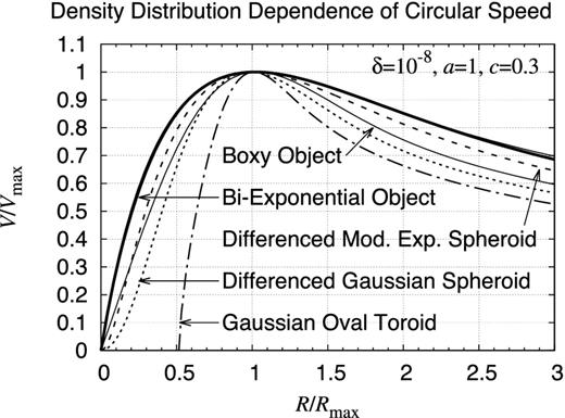
Density distribution dependence of rotation curve. Compared are the rotation curves of eight axisymmetric objects: (i) the bi-exponential object, (ii) the flared bi-exponential object, (iii) the radially exponential and the vertically secant-hyperbolic-function-squared object, (iv) the radially exponential and the vertically Gaussian object, (v) the boxy object, (vi) the differenced modified exponential spheroid, (vii) the differenced Gaussian spheroid, and (viii) the Gaussian oval toroid. Plotted are the rotation curves when a = 1 and c = 0.3 while the velocity V and the radius R are normalized by the maximum speed Vmax and the location of maximum speed Rmax, respectively. Once this normalization is applied, almost invisible is the difference among the first four objects.
![Auxiliary function A(s). Plotted is the curve of an auxiliary function, A(s) ≡ [F(1/2, 1/2; 3/2; s) − 1]/s for the standard interval, |s| ≤ 1. The function is not analytic at s = 1 despite it is finite as A(1) = π/2 − 1 ≈ 0.57.](https://oup.silverchair-cdn.com/oup/backfile/Content_public/Journal/mnras/462/2/10.1093_mnras_stw1765/2/m_stw1765figa1.jpeg?Expires=1750253680&Signature=UYAdGokCbhqSbo~zoH4Ef6Dpkiw-GaNRpwIKlkWWMl0uCYqaFVcxRfnJl0QTWFoPG0-yX7w99N85u4YlFnCp~HxY09CwGdg5S-7hayacG7qSoeKDWYrPQ6mBrO7~iopZfFCMblJX0RHzYYwtPIM10t674yM5-FXyi0Ey4IT0iE1KjOOoq9fBolEQfPyxnQXXyDVXnikJHLn7-KDB8s-3eRs4s~pjL-2ZMxK3yHXsmM9vsub9-KsBXDe03~Rw8fLDJK7~JDlXFDRWv~~Q-R-40-AGdv-sv2fyrcPYALVFKj8dFcojr0mvCRdKjeDQmabwVNbACyTgMAnP~vqKvkaghQ__&Key-Pair-Id=APKAIE5G5CRDK6RD3PGA)
Auxiliary function A(s). Plotted is the curve of an auxiliary function, A(s) ≡ [F(1/2, 1/2; 3/2; s) − 1]/s for the standard interval, |s| ≤ 1. The function is not analytic at s = 1 despite it is finite as A(1) = π/2 − 1 ≈ 0.57.
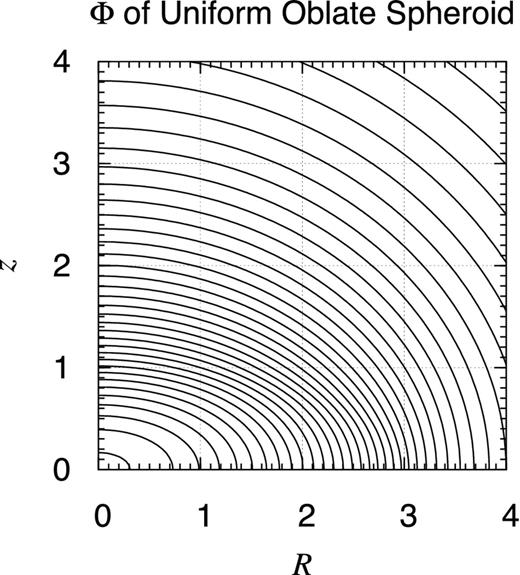
Potential contour map of uniform oblate spheroid. Plotted are the contours of the gravitational potential of a uniform spheroid with the semi-axes, a = 3 and c = 1. The contours are drawn at every 1 per cent level of the bottom value realized at the coordinate centre. The potential is not analytic on the surface of the spheroid where R2/a2 + z2/c2 = 1, although the non-analyticity is not obvious at this scale.

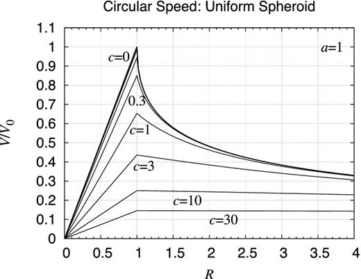
Rotation curve: uniform spheroid. Shown are the rotation curves of uniform spheroids of various values of c as c = 0.003, 0.01, 0.03, 0.1, 0.3, 1.0, 3.0, 10.0, and 30.0 while a is fixed as a = 1. The normalization constant V0 is adjusted such that the total mass of the object becomes the same. As a result, the limit curve of R → ∞ becomes the same, namely that of a point mass. At this scale, invisible is the departure of the curves when c ≤ 0.03 from the limit of c = 0. All the curves have a kink at the surface of the spheroid, namely when R = a.
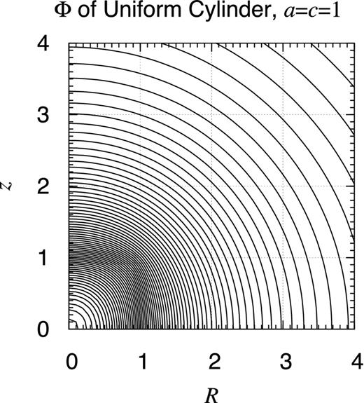
Potential contour map of finite uniform cylinder. Same as Fig. 25 but for a finite uniform cylinder of the radius a = 1 and the half height c = 1. Namely, the object occupies the volume defined as 0 ≤ R ≤ a and 0 ≤ |z| ≤ c. The contours are drawn at every 2 per cent level of the bottom value. Easily visible is the non-analyticity of the potential on the surface of the cylinder, R = a and/or |z| = c. The map is not symmetric with the 90° rotation.
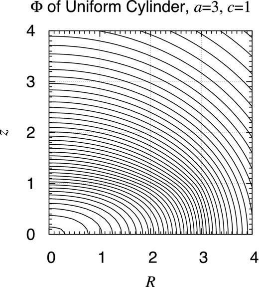
Potential contour map of finite uniform cylinder, a = 3 and c = 1. Same as Fig. D1 but when a = 3 and c = 1.

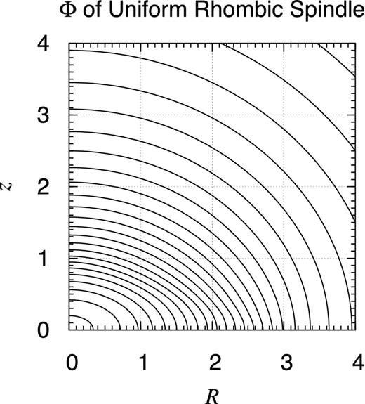
Potential contour map of finite uniform rhombic spindle. Same as Fig. D1 but for a finite uniform rhombic spindle of the radial and vertical semi-axes, a = 3 and c = 1, respectively. Namely, the object occupies the volume defined as 0 ≤ R/a + |z|/c ≤ 1.
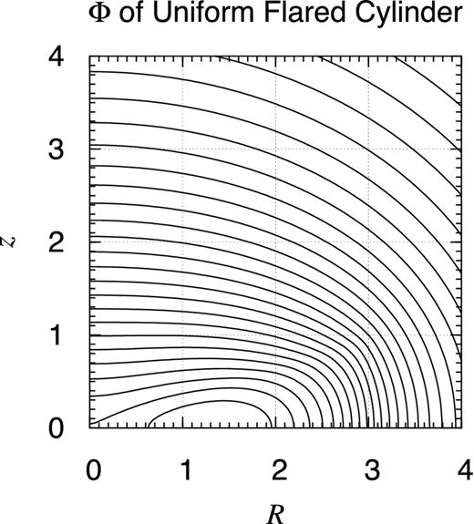
Potential contour map of finite uniform flared cylinder. Same as Fig. D1 but for a finite uniform flared cylinder of the radial and vertical semi-axes, a = 3 and c = 1, respectively. Namely, the object occupies the volume defined as 0 ≤ R/a ≤ |z|/c ≤ 1.
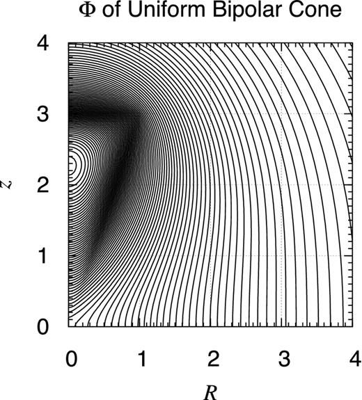
Potential contour map of finite uniform bipolar cone. Same as Fig. D1 but for a finite uniform bipolar cone of the radial and vertical semi-axes, a = 1 and c = 3, respectively. Namely, the object occupies the volume defined as 0 ≤ |z|/c ≤ R/a ≤ 1.
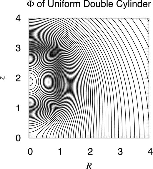
Potential contour map of pair of finite uniform cylinders. Same as Fig. D1 but for a pair of cylinders with the radius and the half height as a = c = 1 and separated by Δz = 2. Namely, the objects occupy the volume defined as 0 ≤ R ≤ a and 0 ≤ |z ± Δz| ≤ c.
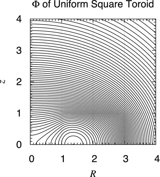
Potential contour map of finite uniform square toroid. Same as Fig. D1 but for a finite uniform square toroid of the inner and outer radii, Rin = 1 and Rout = 3. Namely, the object occupies the volume defined as Rin ≤ R ≤ Rout and 0 ≤ |z| ≤ (Rout − Rin)/2.
![Potential contour map of finite circular uniform toroid. Same as Fig. D1 but for a finite uniform toroid of the inner and outer radii, Rin = 1 and Rout = 3, respectively. Namely, the object occupies the volume defined as 0 ≤ [R − (Rin + Rout)/2]2 + z2 ≤ [(Rout − Rin)/2]2. Thus, centre of the cross-section of the toroid is at R = 2 and z = 0. Meanwhile, the location of the potential maximum is at R ≈ 1.45 and z = 0.](https://oup.silverchair-cdn.com/oup/backfile/Content_public/Journal/mnras/462/2/10.1093_mnras_stw1765/2/m_stw1765figd9.jpeg?Expires=1750253680&Signature=rXQh9Emo~UrzKmFbGpF1BJwmUkYYxxjAR4LjoESwRedHT9qkeK2yf9-ePxkvn9YThMUe82~-1e0UrqQqYAeW1rdaHxB~Q2y9Uc1750wrXYljfjrxgZnjfnIU6aKjATR~numHTL1dzI7E4OKLmDkZPsAMXNxFq1yqW~oUNCslKHER6OhDrsR~s60dU9-sHaPoS0seVTPOfD4EMBn6ZewhUUJtlU-5oBi-sbmtX1xkeTGws4Rk24r7cUP1ZotHdFp0taaOmvFJIvzeAdv~8CElxu6Cuh30TfM9FC2nPo~LdLeWGYvLf0Ave7M9SuQwLqVOG8dru2vfUZ2KbdJ3p8O2pw__&Key-Pair-Id=APKAIE5G5CRDK6RD3PGA)
Potential contour map of finite circular uniform toroid. Same as Fig. D1 but for a finite uniform toroid of the inner and outer radii, Rin = 1 and Rout = 3, respectively. Namely, the object occupies the volume defined as 0 ≤ [R − (Rin + Rout)/2]2 + z2 ≤ [(Rout − Rin)/2]2. Thus, centre of the cross-section of the toroid is at R = 2 and z = 0. Meanwhile, the location of the potential maximum is at R ≈ 1.45 and z = 0.
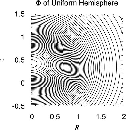
Potential contour map of finite uniform hemisphere. Same as Fig. D1 but for a finite uniform hemisphere of the radius a = 1. Namely, the object occupies the volume defined as 0 ≤ R2 + z2 ≤ a2 and 0 ≤ z.
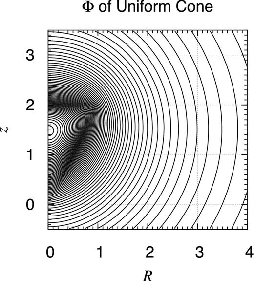
Potential contour map of finite uniform cone. Same as Fig. D1 but for a finite uniform cone of the radius a = 1 and the height c = 2. Namely, the object occupies the volume defined as 0 ≤ z/c ≤ R/a ≤ 1.

Rotation curve: finite uniform cylinder. Shown are the rotation curves of finite uniform cylinders of the radius a and the half height c. Depicted are the results for various values of c as c = 0.003, 0.01, 0.03, 0.1, 0.3, 1.0, 3.0, 10.0, and 30.0 while a is fixed as a = 1. The normalization constant V0 is adjusted such that the total mass of the object is the same. As a result, the limit curve of R → ∞ becomes the same, namely that of a point mass. At this scale, invisible is the departure of the curves when c ≤ 0.03 from the limit of c = 0, namely that of the infinitely thin uniform disc (Fukushima 2016, fig. 5). The curves have a kink at the surface of the cylinder, namely when R = a. The kink approaches to a logarithmic blow-up singularity when c → 0.

Rotation curve: finite uniform rhombic spindle. Same as Fig. D12 but for finite uniform rhombic spindles.
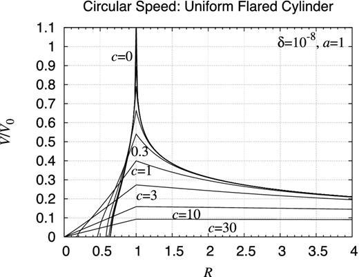
Rotation curve: finite uniform flared cylinder. Same as Fig. D12 but for finite uniform flared cylinders.
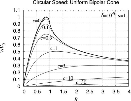
Rotation curve: finite uniform bipolar cone. Same as Fig. D12 but for finite uniform bipolar cones.
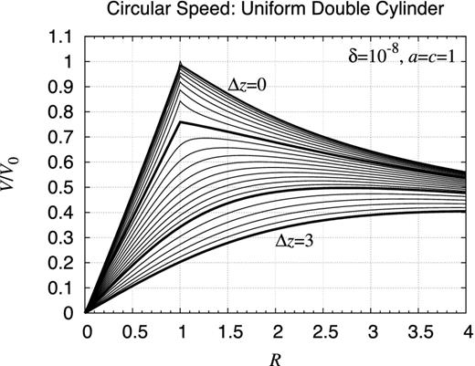
Rotation curve: finite uniform double cylinder. Same as Fig. D7 but for the rotation curve for several values of Δz as Δz = 0.0, 0.1, 0.2, 0.3, 0.4, 0.5, 0.6, 0.7, 0.8, 0.9, 1.0, 1.1, 1.2, 1.3, 1.4, 1.5, 1.6, 1.7, 1.8, 1.9, 2.0, 2.2, 2.4, 2.6, 2.8, and 3.0 while the radius and the half height are fixed as a = c = 1.
5 CONCLUSION
By extending the previous work on an infinitely thin axisymmetric disc (Fukushima 2016), we developed a new method to compute the gravitational potential and the associated acceleration vector of general axisymmetric objects. The method consists of (i) the numerical evaluation of the double integral transform of a given volume mass density by the split quadrature method employing the DE rules, and (ii) the numerical differentiation of the numerically integrated potential by Ridder's algorithm. The comparison with the exact analytical solutions confirms the 13- and 11-digit accuracy of the potential and acceleration computed by the new method in the double precision environment. Although the new method requires the quadrature of double integrals, its CPU time is not so large such as 0.4–2.3 ms for a single point potential computation executed at an ordinary PC. Using the new method, we presented the potential contour map and/or the rotation curves of various kinds of axisymmetric objects including an X/peanut-shaped Galaxy like NGC 128 and finite power-law protoplanetary disc with a central hole such as associated with TW Hya. The new method is immediately applicable to the electrostatic field, and will be easily adapted to the magnetostatic field of general axisymmetric objects.
The fortran 90 programs of the new method are electronically available from the following author's website:
https://www.researchgate.net/profile/Toshio_Fukushima/
The author appreciates the referee's valuable advices to improve the quality of the present paper.
MacMillan (1930) has adopted the negative potential convention as V ≡ −Φ.
REFERENCES
APPENDIX A: GRAVITATIONAL FIELD OF FINITE UNIFORM SPHEROID
A1 Introduction
In the special cases of spheroids whether being oblate or prolate, these elliptic integrals reduce to the elementary functions, namely the inverse trigonometric and/or logarithm functions (MacMillan 1930, section 39, equations 2 and 4). See also Danby (1988, section 5.5) and Binney & Tremaine (2008, tables 2.1 and 2.2). Thus, in principle, it is automatic to obtain the gravitational potential and the acceleration vector of the spheroids.
However, misprints and typos are frequently found in the existing literature. For example, incorrect are the signs of the first terms of the formulas given in Eric Weisstein's World of Physics (Weisstein 2016) despite that its explanation already pointed some typos in a standard textbook.
Also, the original expressions (MacMillan 1930, section 39, equations 2 and 4) suffer from a heavy cancellation when a ≈ c. The same thing would be said for the resulting expressions of the acceleration vector, which are not found in the existing literature.
In order to avoid this problem, Danby (1988, p. 106) obtained the first few terms of the series expansion of the internal potential expression with respect to the deviation from the sphere. This is educative but not enough for precise computation. Therefore, we present below the complete solutions in a unified and cancellation-free form.
A2 External potential
At any rate, it is obvious that the external potential expression in equation (A12) is never written as a scalar function of a homogeneous quadratic polynomial of R and z such as R2/α2 + z2/γ2. In other words, this is a good specimen that, even if an object is spheroidally symmetric, its gravitational potential is not spheroidally symmetric in general.
A3 Auxiliary function
A4 Internal potential
A5 Spherical limit
A6 Acceleration vector
This is a surprisingly simple result as MacMillan (1930, section 39) stressed
... Although κ is a function of x, y, and z, it is not necessary to regard it as such in forming the first partial derivatives of V with respect to x, y, and z; for it was shown in Section 36 that even for the general ellipsoid the derivative of the potential with respect to x, y, and z, in so far as these variables are involved implicitly through κ, vanishes...
A7 Rotation curve
A8 Sketches
For the readers’ understanding, we present Figs A2 and A3 depicting the contour map of the gravitational potential of a pair of uniform spheroids with semi-axes as (i) a = 3 and c = 1, and (ii) a = 1 and c = 3. Also, we plot the rotation curves of uniform spheroids with various aspect ratios in Fig. A4.
APPENDIX B: HINTS FOR PARALLEL INTEGRATION
In fact, in the actual execution of the parallel integration utilizing the OpenMP architecture, we (i) prepare several sets of copies of the DE quadrature programs, intde and intdei, beforehand, and (ii) assign a differently numbered set of the DE quadrature programs to a different computing unit by using the omp sections block and multiple omp section statements. This is in order to avoid the fatal modification of intermediate results during the random calling of the same child subprogram by multiple parent subprograms.
A sample fortran code of the resulting parallel evaluation of the double integral is
real*8 function phiint(r,z)
...
common /param1/r1,z1,rp1
common /param2/r2,z2,rp2
common /param3/r3,z3,rp3
common /param4/r4,z4,rp4
...
r1=r; z1=z; r2=r; z2=z; r3=r; z3=z; r4=r; z4=z
...
!$omp parallel
!$omp sections
!$omp section
call intder1(psiint1,0.d0,r,eps,phi1,err1)
!$omp section
call intdeir1(psiint2,r,eps,phi2,err2)
!$omp section
call intder2(psiint3,0.d0,r,eps,phi3,err3)
!$omp section
call intdeir2(psiint4,r,eps,phi4,err4)
!$omp end sections
!$omp end parallel
phiint=phi1+phi2+phi3+phi4
return; end
where the statements including ‘$omp’ are OpenMP directives for fortran.
The line integral computation is conducted by differently named but essentially the same subprograms as
real*8 function psiint1(rp)
...
common /param1/r1,z1,rp1
rp1=rp
call intdeiz1(fint1,-z1,eps1,psiint1,err1)
return; end
real*8 function psiint2(rp)
...
common /param2/r2,z2,rp2
rp2=rp
call intdeiz2(fint2,-z2,eps2,psiint2,err2)
return; end
real*8 function psiint3(rp)
...
common /param3/r3,z3,rp3
rp3=rp
call intdeiz3(fint3,z3,eps3,psiint3,err3)
return; end
real*8 function psiint4(rp)
...
common /param4/r4,z4,rp4
rp4=rp
call intdeiz4(fint4,z4,eps4,psiint4,err4)
return; end
where intdeiz1, intdeiz2, intdeiz3, and intdeiz4 are the same subprogram as intdei but named differently.
Also, the integrand is computed by almost the same functions, fint1, fint2, fint3, and fint4. They are, after setting G = 1 by adopting an appropriate unit system, defined as
real*8 function fint1(zp)
real*8 zp,r1,z1,rp1,rho1,green1
common /param1/r1,z1,rp1
fint1=-rho1(rp1,-zp)*green1(rp1,-zp,r1,z1)
return; end
real*8 function fint2(zp)
real*8 zp,r2,z2,rp2,rho2,green2
common /param2/r2,z2,rp2
fint2=-rho2(rp2,-zp)*green2(rp2,-zp,r2,z2)
return; end
real*8 function fint3(zp)
real*8 zp,r3,z3,rp3,rho3,green3
common /param3/r3,z3,rp3
fint3=-rho3(rp3,zp)*green3(rp3,zp,r3,z3)
return; end
real*8 function fint4(zp)
real*8 zp,r4,z4,rp4,rho4,green4
common /param4/r4,z4,rp4
fint4=-rho4(rp4,zp)*green4(rp4,zp,r4,z4)
return; end
where (i) rho1 through rho4 are differently named but essentially the same functions to calculate the volume mass density profile, ρ(R′, z′), while (ii) green1 through green4 are differently named but actually the same functions to return the azimuthally integrated Green's function, g(R′, z′; R, z), as specified in equation (17). We warn the readers that fint1 and fint2 are the same functions but numbered differently, both of which are to compute the integrand for −z, while fint3 are fint4 are a similar pair for +z. This difference in the argument sign was necessary because Ooura's intdei is designed to evaluate an integral over a positively open semi-infinite interval such as t0 ≤ t < +∞.
In this example, the named common blocks are carefully distributed to the subprograms so as to avoid the interference among them during the parallel execution of subprograms. This is another important point to guarantee the correctness of the parallel computation.
APPENDIX C: GRAVITATIONAL FIELD OF MIYAMOTO–NAGAI MODEL
APPENDIX D: GRAVITATIONAL FIELD OF FINITE UNIFORM OBJECTS
Here, we present the contour map of the gravitational potential and/or the rotation curve of a series of finite uniform axisymmetric objects. Although such objects are rarely found in nature, the information on their gravitational fields will give us some hints on those of inhomogeneous objects with similar shapes.
Figs D1–D11 illustrate the contour map of the gravitational potential of these objects computed by the new method when the parameters are chosen as a = 1 or 3, c = 1, 2, or 3, and ξ0 = η0 = 2. The shape of the potential contours is significantly different from that of the density contours. In general, the potential contours approach to circles when the distance from the object increases. This is a natural consequence that, independently of its shape, the point mass potential becomes a good approximation of the finite object for the evaluation points when |$r \equiv \sqrt{R^2+z^2} \rightarrow \infty$|. Also, the cross-sections of the object surfaces are sometimes visible as the dense concentration of contours since the potential is not analytic there.
Meanwhile, Fig. D12 compares the rotation curves of the non-flared cylinders for various values of c as c = 0.003, 0.01, 0.03, 0.1, 0.3, 1, 3, 10, and 30 while a is fixed as a = 1. In drawing Fig. D12, we normalized the computed circular speed such that their asymptotic forms are the same as that of a point of the same total mass. Similarly, Figs D13–D18 indicate the rotation curves of other uniform objects with the plane symmetry. These rotation curves exhibit kinks when crossing the surface of the object if it lies on the z-plane.
In some cases, the rotation curve blows up infinitely at the kink point. This happens for infinitely thin cylinders with and/or without flaring. It is noteworthy that the imaginary circular speed is realized in an inner region for toroidal objects and some flared cylinders. Refer to Figs D14, D17, and D18. This is not unphysical situation. It simply means that the gravitational attraction from the external mass is stronger than that from the internal one.

Rotation curve: finite uniform circular toroid. Same as Fig. 38 but for a uniform circular toroid for several values of Rin as Rin = 0.1, 0.2, 0.3, 0.4, 0.5, 0.6, 0.7, 0.8, 0.9, 1.0, 1.1, 1.2, 1.3, 1.4, 1.5, 1.6, 1.7, 1.8, and 1.9, and the outer radius is fixed as Rout = 2. Meanwhile, the half height is arranged as c ≡ (Rout + Rin)/2 such that the cross-section is square-shaped. All the curves have a kink at R = Rout.
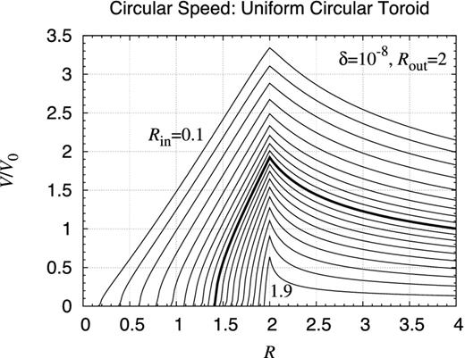
Rotation curve: finite uniform circular toroid. Same as Fig. 38 but for a uniform circular toroid for several values of Rin as Rin = 0.1, 0.2, 0.3, 0.4, 0.5, 0.6, 0.7, 0.8, 0.9, 1.0, 1.1, 1.2, 1.3, 1.4, 1.5, 1.6, 1.7, 1.8, and 1.9, while the outer radius is fixed as Rout = 2. All the curves have a kink at R = Rout.
APPENDIX E: GRAVITATIONAL FIELD OF INFINITELY EXTENDED SPHEROIDS
Although the gravitational fields for general spheroids are computable by another approach (Binney & Tremaine 2008, section 2.5.2), we present the contour map of the gravitational potential and the rotation curve of some spheroids below. This is because most of the information is rarely accessible in the literature.
In the Besançon galactic model (Robin et al. 2003, table 3), the Gaussian and the modified exponential spheroids are used in representing the thin disc of young and old stars. The Sérsic spheroid with the index 4 is nothing but the de Vaucouleurs spheroid (de Vaucouleurs 1948, 1953). Also, the Einasto spheroids with the index 1/2 and 1 are, except the radial scaling factor, the same as the Gaussian and exponential spheroids, respectively.
![Density profile of some spheroids. Plotted are the volume mass density of some spheroids: (i) the Gaussian spheroid, ρG(s) ≡ ρ0 exp (−s2), where $s \equiv \sqrt{(R/a)^2+(z/c)^2}$, (ii) the exponential spheroid, ρX(s) ≡ ρ0 exp (−s), (iii) the modified exponential spheroid, $\rho _{\rm M} (s) \equiv \rho _0 \exp \left[ - s^2 \left/ \left( 1 + \sqrt{1+s^2} \right) \right] \right.$, and (iv) the Burkert spheroid (Burkert 1995), ρB(s) ≡ ρ0(1 + s)−1(1 + s2)−1. The thick curve shows the Gaussian spheroid. The exponential and Burkert spheroids have a cusp at the coordinate centre.](https://oup.silverchair-cdn.com/oup/backfile/Content_public/Journal/mnras/462/2/10.1093_mnras_stw1765/2/m_stw1765fige1.jpeg?Expires=1750253681&Signature=rtHQfXfgDvidoBUCu2lB27T5zp-1LB5~U4fVCSjMK7yxF09Rg56To0Nvk92Y0l5n4b2azv8olASjkNs79bZuY8fYCcEHTPuQps4RY5t7e2-XO~bMLqEFol0AXWlv10NknPnIQcaAOMfuIVAf~XoexSpi8y41RTn7kA07oKzasCyObKZjYwCuF9idci8DBKtoGWERIae1vAwZ7YoyBKJY5wV6MQ86krnTTLAmeQnkDP-mqng942QKrN8faylz6V75jmhIM~goyUPn1j82UmmrAx9pron---ChjZgAhqLwKl1vv~OcavHObPV9aHfkUoyFWxQM4032IkXV9ZujrXQ9pQ__&Key-Pair-Id=APKAIE5G5CRDK6RD3PGA)
Density profile of some spheroids. Plotted are the volume mass density of some spheroids: (i) the Gaussian spheroid, ρG(s) ≡ ρ0 exp (−s2), where |$s \equiv \sqrt{(R/a)^2+(z/c)^2}$|, (ii) the exponential spheroid, ρX(s) ≡ ρ0 exp (−s), (iii) the modified exponential spheroid, |$\rho _{\rm M} (s) \equiv \rho _0 \exp \left[ - s^2 \left/ \left( 1 + \sqrt{1+s^2} \right) \right] \right.$|, and (iv) the Burkert spheroid (Burkert 1995), ρB(s) ≡ ρ0(1 + s)−1(1 + s2)−1. The thick curve shows the Gaussian spheroid. The exponential and Burkert spheroids have a cusp at the coordinate centre.
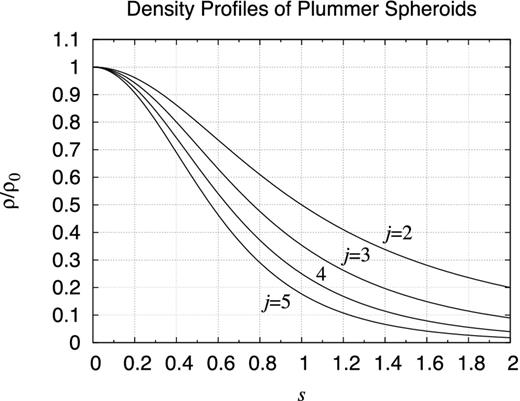
Density profile of indexed Plummer spheroids. Same as Fig. E1 but for some indexed Plummer spheroids, ρPj(s) ≡ ρ0(1 + s2)−j/2, where |$s \equiv \sqrt{(R/a)^2+(z/c)^2}$|. Here (i) the case j = 2 is the modified isothermal model (King 1962), (ii) the case j = 3 is the modified Hubble model (Rood et al. 1972), (iii) the case j = 4 is the perfect spheroid (de Zeeuw 1985a,b), and (iv) the case j = 5 is the original Plummer model (Plummer 1911).

Density profile of double power-law spheroids. Same as Fig. E2 but plotted are double logarithmic graphs for some spheroids with the double power-law density profile: (i) the Jaffe spheroid (Jaffe 1983), ρJ(s) ≡ ρ0s−2(1 + s)−2, where |$s \equiv \sqrt{(R/a)^2+(z/c)^2}$|, (ii) the Hernquist spheroid (Hernquist 1990), ρH(s) ≡ ρ0s−1(1 + s)−3, and (iii) the Navarro–Frenk–White (NFW) spheroid (Navarro, Frenk & White 1997), ρN(s) ≡ ρ0s−1(1 + s)−2. The result of the Jaffe spheroid is depicted in a broken curve while those of the NFW and Hernquist spheroids are shown by a thick and a thin solid curve.
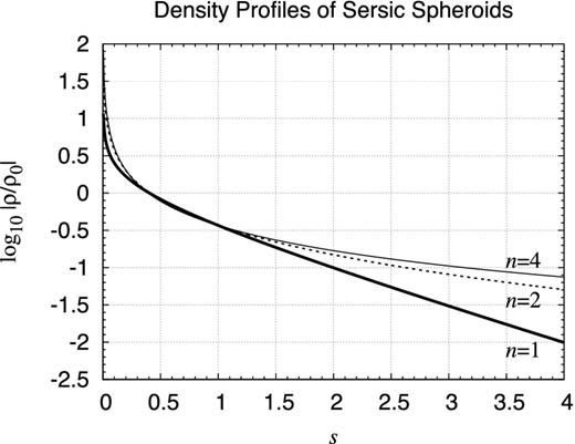
Density profile of Sérsic spheroids. Same as Fig. E2 but plotted are the single logarithmic graphs for the spheroids approximately resulting the Sérsic law of the surface intensity profile (Sérsic 1963, 1968). Here the volume mass density is written as |$\rho _{{\rm S}n} (s) \equiv \rho _0 s^{-p_n} \exp ( - s^{1/n} )$|, where |$s \equiv \sqrt{(R/a)^2+(z/c)^2}$| while the power index pn are approximated (Lima Neto, Gerbal & Márquez 1999) as pn = 1 − 0.6097n + 0.054 63n2. Compared are the curves of (i) n = 1 drawn by a thick line, (ii) n = 2 by a dotted line, and (iii) n = 4 by a thin line. The case of the index n = 4 corresponds to the famous de Vaucouleurs’ law (de Vaucouleurs 1948).
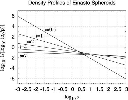
Density profile of Einasto spheroids. Same as Fig. E2 but plotted are modified logarithmic graphs for the Einasto spheroids. Their volume mass density profile is expressed as ρTi(s) ≡ ρ0 exp (−dis1/i), where |$s \equiv \sqrt{(R/a)^2+(z/c)^2}$| while the coefficient di are approximated (Merritt et al. 2006, equation 24) as di = 3i − 1/3 + 0.0079/i. Compared are the curves of some indices as n = 1/2, 1, 2, 4, and 7. Except the scaling constants, the curves of n = 1/2 and 1 are the same as those of the Gaussian and exponential spheroids, respectively.
The adopted formulas of pn and di are of approximate nature. However, through independent numerical deprojection of the surface intensity curves for pn and numerical solutions of a non-linear equation involving the incomplete gamma functions for di, we confirm that they are sufficiently precise for the purpose to draw the contour maps and the rotation curves.
Even if the volume mass density profiles are spheroidally symmetric, the resulting gravitational potentials are not so. Therefore, the two-dimensional distribution of the gravitational potential is indispensable in order to understand its global behaviour. Figs E6–E22 show the contour maps of the gravitational potentials of these spheroids while the semi-axes are fixed the same as a = 1 and c = 0.3. Although the contours in these maps are not genuine ellipses, their departure from ellipses is difficult to notice.
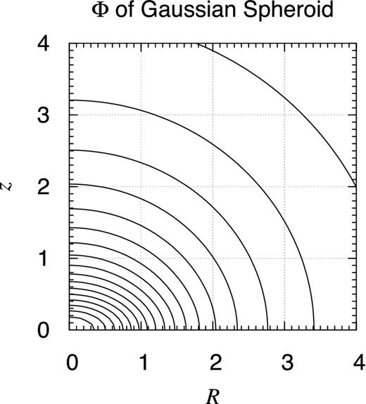
Potential contour map of Gaussian spheroid. Shown is the contour map of the gravitational potential of the Gaussian spheroid defined as ρG(s) ≡ ρ0 exp (−s2) while |$s \equiv \sqrt{(R/a)^2+(z/c)^2}$| when a = 1 and c = 0.3. The contours are drawn at every 5 per cent level of the bottom value realized at the coordinate origin. Despite their elliptical outlook, the contours are not genuine ellipses.
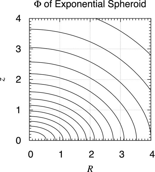
Potential contour map of exponential spheroid. Same as Fig. E6 but for the exponential spheroid defined as ρX(s) ≡ ρ0 exp (−s) while |$s \equiv \sqrt{(R/a)^2+(z/c)^2}$| when a = 1 and c = 0.3.
![Potential contour map of modified exponential spheroid. Same as Fig. E6 but for the modified exponential spheroid (Robin et al. 2003) defined as $\rho _{\rm M} (s) \equiv \rho _0 \exp [ - s^2/ \sqrt{1 + \sqrt{1+s^2}} ]$ while $s \equiv \sqrt{(R/a)^2+(z/c)^2}$ when a = 1 and c = 0.3.](https://oup.silverchair-cdn.com/oup/backfile/Content_public/Journal/mnras/462/2/10.1093_mnras_stw1765/2/m_stw1765fige8.jpeg?Expires=1750253681&Signature=XtNq2FC9UexWX4LD38CnECzkEVEA6t3QBOvE0bIeesnvxvgNDk7RdtZL0CIcA8G7q7ZavJ9VHEmm1FQhH1D~r0o4hcx3J05821NXtzsvc8bApadfR4K7N3tC2b-uaU3YpnbMV5cx7KP8sKg-NYqfz3qF1G1SPV2BVCvVG3GaWFSgIfCLhHCLxAaHDdIlKsFmP2rzZpGx~4xb8LCet4z5QAfRc5Z3o61XWkBNvxh112HqHpbGn8ZfUAUHY-0KprIj2sjqc-QlCOWeHc7AJX66GyCRvnLBs2gXDqBrp8h4uNTIAeDDM15H5PcFxjH~K7MqV~xynysyZA8V~PDJWX8V9w__&Key-Pair-Id=APKAIE5G5CRDK6RD3PGA)


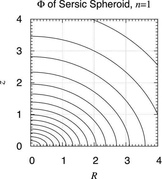
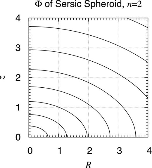
Potential contour map of Sérsic spheroid, n = 2. Same as Fig. E6 but for a Sérsic spheroid (Sérsic 1963, 1968) of index n = 2 defined as |$\rho _{{\rm S}2} (s) \equiv \rho _0 s^{-p_2} \exp \left( - \sqrt{s} \right)$| while |$s \equiv \sqrt{(R/a)^2+(z/c)^2}$| and p2 ≈ 0.708 807 50 when a = 1 and c = 0.3.
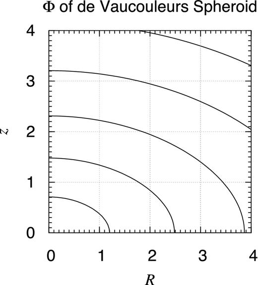
Potential contour map of de Vaucouleurs spheroid. Same as Fig. E6 but for a de Vaucouleurs spheroid (de Vaucouleurs 1948), namely Sérsic spheroid of index n = 4 defined as |$\rho _{{\rm S}4} (s) \equiv \rho _0 s^{-p_4} \exp \left( - s^{1/4} \right)$| while |$s \equiv \sqrt{(R/a)^2+(z/c)^2}$| and p4 ≈ 0.850 989 37 when a = 1 and c = 0.3.
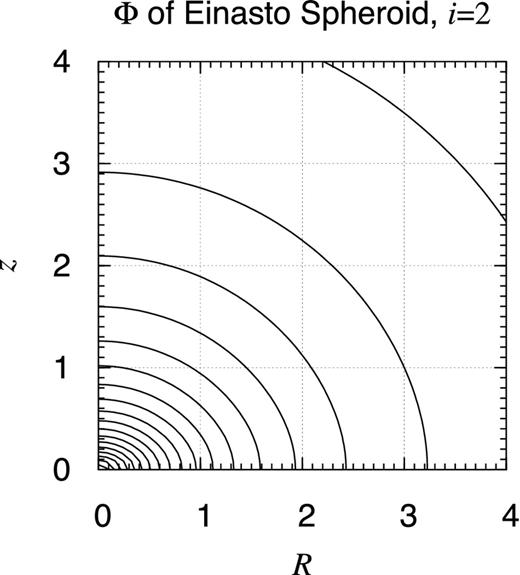


More visible is the difference in the spatial distribution of the contour levels, namely the radial and/or vertical distribution of the variation of the potential such as the circular speed on the symmetric plane as shown in Figs E23–E39. The rotation curves of these spheroids are depicted there for several values of c as c = 0.1, 0.2, 0.3, 0.4, 0.5, 0.6, 0.7, 0.8, 0.9, 1, 1.5, 2, 2.5, 3, 3.5, 4, 4.5, and 5 while a is fixed as a = 1. Obviously, the functional form of the rotation curve is significantly different spheroid by spheroid. For example, almost flat rotation curves are produced by the modified isothermal spheroids. This situation is mostly the same as the Mestel disc in the case of infinitely thin axisymmetric discs (Mestel 1963). Also, the Jaffe spheroids give the finite value of the circular speed at the object centre, although it is unphysical.

Rotation curve of Gaussian spheroid. Shown are the rotation curves of a group of spheroids with the volume mass density expressed as ρG(s) ≡ ρ0 exp (−s2), where |$s \equiv \sqrt{(R/a)^2 + (z/c)^2}$|. Plotted are the curves for various values of c as c = 0.1, 0.2, 0.3, 0.4, 0.5, 0.6, 0.7, 0.8, 0.9, 1, 1.5, 2, 2.5, 3, 3.5, 4, 4.5, and 5 while a is set as a = 1 and the nominal density value, ρ0, is fixed. If the total mass is fixed instead, V0 is adjusted such that the asymptotic forms of all the curves become the same. The thick curve represents the spherically symmetric case, c = a, which is analytically computable by means of the error function.
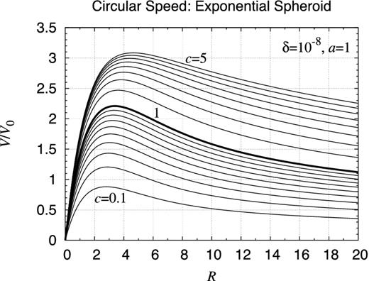
Rotation curve of modified exponential spheroid. Same as Fig. E23 but for a spheroid with the volume mass density expressed as ρX(s) ≡ ρ0 exp (−s), where |$s \equiv \sqrt{(R/a)^2+(z/c)^2}$|.
![Rotation curve of modified exponential spheroid. Same as Fig. E23 but for a spheroid with the volume mass density expressed as $\rho _{\rm M} (s) \equiv \rho _0 \exp [- 2 s^2/( 1 + \sqrt{1+4s^2} ) ]$, where $s \equiv \sqrt{(R/a)^2+(z/c)^2}$.](https://oup.silverchair-cdn.com/oup/backfile/Content_public/Journal/mnras/462/2/10.1093_mnras_stw1765/2/m_stw1765fige25.jpeg?Expires=1750253681&Signature=xnq3If5GGJvWYliAQOAz1soy-kA4kb5-k2mxjIlIcUWnhfmGlqzI1EReUBmqhbsjoRB48Vt2aHAMhnXZdBoDhGh1CMnxsPdw-QAXr11Nq62DGPZExdzUXmiOzXMLucNQp67XZ1Sf2raBhrV-j-2Xik7h1FKCtglGx45AFQGpW0MUUQZ4UD9TOPNgZncA7KHSWU3yuoy1B9sFf0iUaDg0JtHDSZ1Ax~iGVqzcMMN3H4TsXWyHzM1E-FAutDiK9ACrel~hvwKaBgz9VJqLA-wLcraLZ1WCA5T97J754MDImerC5JradiwahyxqPhmdRkq7LXKhGr5SUiuS30zOBzMVVA__&Key-Pair-Id=APKAIE5G5CRDK6RD3PGA)
Rotation curve of modified exponential spheroid. Same as Fig. E23 but for a spheroid with the volume mass density expressed as |$\rho _{\rm M} (s) \equiv \rho _0 \exp [- 2 s^2/( 1 + \sqrt{1+4s^2} ) ]$|, where |$s \equiv \sqrt{(R/a)^2+(z/c)^2}$|.


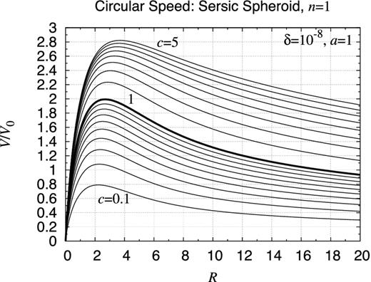
Rotation curve of Sérsic spheroid, n = 1. Same as Fig. E23 but for a spheroid with the volume mass density expressed as |$\rho _{{\rm S}1} (s) \equiv \rho _0 s^{-p_1} \exp (-s)$|, where p1 ≈ 0.444 930 00 and |$s \equiv \sqrt{(R/a)^2+(z/c)^2}$|. This density profile approximately reproduces the surface brightness profile following the Sérsic law of index n = 1 (Sérsic 1963, 1968).
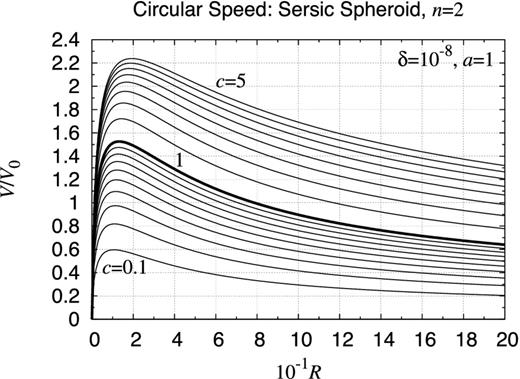
Rotation curve of Sérsic spheroid, n = 2. Same as Fig. E23 but for a spheroid with the volume mass density expressed as |$\rho _{{\rm S}2} (s) \equiv \rho _0 s^{-p_2} \exp \left( - \sqrt{s} \right)$|, where p2 ≈ 0.708 807 50 and |$s \equiv \sqrt{(R/a)^2+(z/c)^2}$|. Enlarged is the range of radial distance so as to cover the feature of rise and fall.
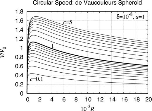
Rotation curve of de Vaucouleurs spheroid. Same as Fig. E23 but for a spheroid with the volume mass density expressed as |$\rho _{{\rm S}4} (s) \equiv \rho _0 s^{-p_4} \exp \left( - s^{1/4} \right)$|, where p4 ≈ 0.850 989 37 and |$s \equiv \sqrt{(R/a)^2+(z/c)^2}$|. This time, further extended is the range of radial distance so as to cover the feature of rise and fall. If the object is spherically symmetric such that a = c, the volume density profile approximately reproduces the surface brightness profile following the de Vaucouleurs’ law (de Vaucouleurs 1948).
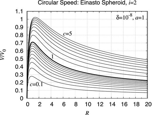
Rotation curve of Einasto spheroid, i = 2. Same as Fig. E23 but for a spheroid with the volume mass density expressed as ρE2(s) ≡ ρ0 exp (−d2 s), where d2 ≈ 5.706 1667 and |$s \equiv \sqrt{(R/a)^2+(z/c)^2}$|.
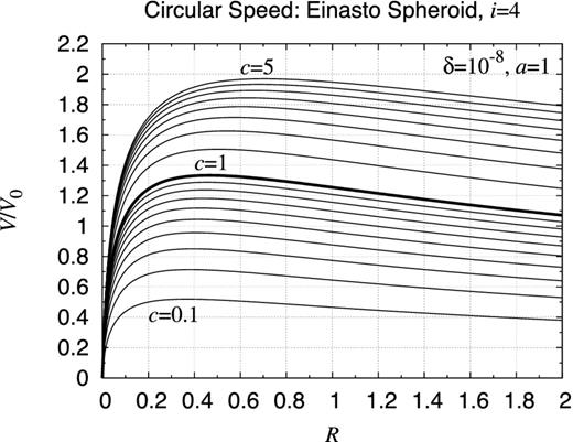
Rotation curve of Einasto spheroid, i = 4. Same as Fig. E23 but for a spheroid with the volume mass density expressed as ρE4(s) ≡ ρ0 exp (−d4s1/4), where d4 ≈ 11.686 417 and |$s \equiv \sqrt{(R/a)^2+(z/c)^2}$| (Einasto 1965). This time, the radial argument range is diminished so as to emphasize the initial rising feature.
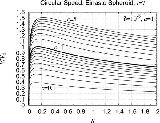
Rotation curve of Einasto spheroid, i = 7. Same as Fig. E23 but for a spheroid with the volume mass density expressed as ρE7(s) ≡ ρ0 exp (−d7s1/7), where d7 ≈ 20.677 952 and |$s \equiv \sqrt{(R/a)^2+(z/c)^2}$| (Einasto 1965). Again, the radial argument range is diminished so as to emphasize the initial rising feature.
Except these two cases, all the other rotation curves (i) initially rise as a linear function, (ii) reach the maximum value when 0.1 < R/a < 6, and (iii) decay monotonically. The differences are in (i) the inclination of the initial rise, (ii) the location of the peak, and (iii) the decreasing manner when R → ∞. Refer to Fig. E40 showing the rotation curves after their peak values and the location of peaks become the same by appropriate scaling. See also Table E1 for a quantitative comparison.
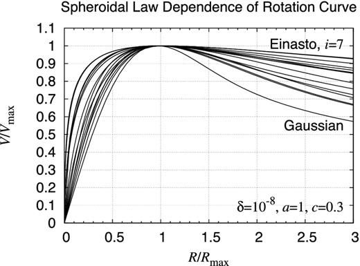
Spheroidal law dependence of rotation curve. Same as Fig. 47 but compared are the rotation curves of most of the spheroids when a = 1 and c = 0.3. The exceptions are (i) the Jaffe spheroid where the curve reaches the maximum at the coordinate origin, and (ii) the modified isothermal spheroid where the curve increases monotonically and no maximum value is attained. Among the curves shown here, that of the Einasto spheroid of the index i = 7 increases most quickly and decreases most gradually. Meanwhile, that of the Gaussian spheroid grows most slowly and decays most rapidly. See Table E1 for the detailed comparison.
Rotation curve indices of spheroids. Summarized are the numerical values of two indices of the rotation curve, W1/2 and W2, for a group of infinitely extended spheroids when c/a = 0.3. The rotation curve index for a real-valued factor, k, is defined as Wk ≡ V(kRmax)/Vmax, where (i) Vmax ≡ max RV(R) is the peak value of the circular speed, and (ii) Rmax is the location of the peak such that Vmax = V(Rmax). The spheroids are listed in the increasing order of W1/2. Although this shows a special case when c/a = 0.3, we experimentally confirmed that the order is hardly sensitive to the aspect ratio.
| Spheroid | W1/2 | W2 |
|---|---|---|
| Gaussian | 0.773 | 0.726 |
| Plummer | 0.817 | 0.864 |
| Modified exponential | 0.834 | 0.836 |
| Exponential | 0.853 | 0.830 |
| Perfect | 0.860 | 0.878 |
| Sérsic (n = 1) | 0.884 | 0.866 |
| Modified Hubble | 0.890 | 0.930 |
| Sérsic (n = 2) | 0.910 | 0.910 |
| Burkert | 0.911 | 0.936 |
| Hernquist | 0.930 | 0.930 |
| Einasto (i = 2) | 0.936 | 0.938 |
| Navarro–Frenk–White | 0.952 | 0.958 |
| Einasto (i = 4) | 0.954 | 0.947 |
| de Vaucouleurs | 0.968 | 0.972 |
| Einasto (i = 7) | 0.968 | 0.976 |
It is interesting that, for each kind of spheroid, almost flat rotation curves are realized when c/a is large. This is a natural consequence of the facts that (i) very prolate spheroids resemble thin rods, (ii) their gravitational potentials are similar to that of an infinitely thin rod, namely the logarithmic potential (MacMillan 1930) as Φ(R, z) ∝ − ln R, then (iii) the radial acceleration, FR(R, z) ≡ (∂Φ/∂R), is in proportion to 1/R, and therefore, (iv) the rotation curve, |$V(R) \equiv \sqrt{-R F_R(R,0)}$|, becomes asymptotically flat.
Qualitatively speaking, we notice that the overall feature of the rotation curves depends on the aspect ratio c/a rather weakly. Therefore, one may quote the spherically symmetric case, a = c, which is analytically and easily computed thanks to Newton's theorems, as the representative rotation curve. If a better approximation is required for oblate spheroids where 0 ≤ c/a ≤ 1, we suggest a linear interpolation between two major cases: (i) the spherically symmetric case where c/a = 1, and (ii) the infinitely thin case where c/a = 0, the result of which is quickly computed (Fukushima 2016).
