


Abstract
We present a new model of the microwave sky in polarization that can be used to simulate data from cosmic microwave background polarization experiments. We exploit the most recent results from the Planck satellite to provide an accurate description of the diffuse polarized foreground synchrotron and thermal dust emission. Our model can include the two mentioned foregrounds, and also a constructed template of Anomalous Microwave Emission. Several options for the frequency dependence of the foregrounds can be easily selected, to reflect our uncertainties and to test the impact of different assumptions. Small angular scale features can be added to the foreground templates to simulate high-resolution observations. We present tests of the model outputs to show the excellent agreement with Planck and Wilkinson Microwave Anisotropy Probe (WMAP) data. We determine the range within which the foreground spectral indices can be varied to be consistent with the current data. We also show forecasts for a high-sensitivity, high-resolution full-sky experiment such as the Cosmic ORigin Explorer. Our model is released as a python script that is quick and easy to use, available at http://www.jb.man.ac.uk/chervias.
1 INTRODUCTION
Over the past decades, the temperature anisotropies of the cosmic microwave background (CMB) have been an invaluable probe of the cosmological model (e.g. Calabrese et al. 2013; Hinshaw et al. 2013; Planck Collaboration XIII 2015). The design of future CMB experiments is now driven by the goal of measuring accurately the polarization of the CMB, and searching for primordial polarization B modes, a detection which would prove unequivocally the inflationary scenario. However, bright foreground emission due to our Galaxy can jeopardize this measurement, and accurate models of the polarization sky are needed (see e.g. Betoule et al. 2009; Armitage-Caplan et al. 2012; Errard & Stompor 2012; Bonaldi, Ricciardi & Brown 2014; BICEP2/Keck and Planck Collaborations et al. 2015; Remazeilles et al. 2016).
Until recently, full-sky polarization maps of the Galactic emission were based on total intensity measurements and models of the polarization physical properties, angles and polarization fractions (e.g. Miville-Deschenes 2011; O'Dea et al. 2012; Delabrouille et al. 2013). However, the uncertainties in such modelling made it difficult to create polarization templates accurately reproducing the observed morphology in the sky. The recent release of the Planck data has improved this situation, by providing for the first time foreground maps extracted directly from the polarization data (Planck Collaboration X 2015). Before this information can be used to forecast future polarization experiments, however, it is necessary to overcome the limitations due to the Planck resolution and noise levels. Moreover, a suite of foreground models needs to be explored, to reflect the current uncertainties on polarized foregrounds. This is the goal of the current paper, where we deliver a new sky model of diffuse polarized emission in the microwave frequency range, based on the most up-to-date information from Planck.
In contrast to previous work (Delabrouille et al. 2013), the model we present is not a comprehensive model that includes all point-like and diffuse emission in the microwave sky. Instead, we focus on diffuse polarized emission only and aim to provide a simpler and more flexible tool, to allow model selection for forecast purposes, as well as to test and debug data analysis methods on simulated data of varying complexity. We also introduce, for the first time, the capability to vary the foreground morphology for Monte Carlo purposes. We believe that our model, which we provide as a python script, will be a useful tool for the CMB polarization community.
The paper is organized as follows: In Section 2 we describe our sky model; in Section 3 we describe the simulation procedure; in Section 4 we compare the outputs of our model with the most recent polarization data. In Section 5 we discuss the forecast and Monte Carlo capabilities of our sky model and, finally, in Section 6 we draw our conclusions.
2 SKY MODEL
2.1 CMB component
The CMB is generated starting from a set of input Cℓ power spectra from theory: TT (the autospectrum of the total intensity), EE and BB (the two autospectra from the curl-free and divergence-free linear combination fields of polarization intensity), and TE (the cross-spectrum between the total intensity and the polarization curl-free fields). These can be produced starting from a set of cosmological parameters, for example with the camb code (Howlett et al. 2012). The map is generated using the synfast task of healpix1 (Górski et al. 2005). It is then converted from thermodynamic to antenna temperature units at various frequencies with the usual blackbody law with TCMB = 2.725 48 K.
2.2 Foreground templates
The simplest model of diffuse polarized foregrounds that is compatible with the observations has two Galactic polarized foregrounds: synchrotron and thermal dust.
We construct templates of these emission components based on the synchrotron and thermal dust polarization maps extracted from Planck observations with the Bayesian component separation method commander (Planck Collaboration X 2015) and publicly available through the Planck Legacy Archive.2
The synchrotron template has a reference frequency of 30 GHz and a resolution of 40′ full width at half-maximum (FWHM). However, the pixel size of ∼14 arcmin (corresponding to Nside = 256) means that pixelization artefacts are visible on the maps. We eliminated these artefacts by resampling the map, upgrading it to Nside = 512 and smoothing it to a final 1° resolution.
The dust template obtained by Planck Collaboration X (2015) has a reference frequency of 353 GHz and a resolution of 10 arcmin FWHM. Fig. 1 shows both Q intensity templates.

2.2.1 Adding high-ℓ features to the foreground templates
Since the synchrotron and thermal dust templates have finite resolution, they do not have power at small scales. In our models, we would like to simulate high-ℓ power since the real sky thermal dust and synchrotron emissions are expected to have these features.
The approach that we follow is to generate a random map using a suitable power spectrum, based on the extrapolation of the power spectrum of the original map to higher multipoles. Since this procedure involves a random realization, it can be also used to create variations over different foreground maps, for example for Monte Carlo purposes (this aspect is discussed in Section 5).
A common assumption is that the power spectrum of the foreground maps has a power-law behaviour in ℓ. Fig. 2 (top) shows the EE power spectra of the synchrotron template in green. The power-law behaviour is not a good approximation at the highest multipoles, where the slope flattens with respect to lower ℓs. We none the less adopted the power-law approximation and computed the best-fitting slope at the lowest multipoles. We used a least-squares polynomial fit, that minimizes the difference between model and data, added in quadrature within a given multipole range. Our model is a straight line in the log Cℓ–log ℓ space. This procedure also outputs the covariance matrix for the fit parameters, and we adopted the square root of the diagonal terms as errors on each of them.
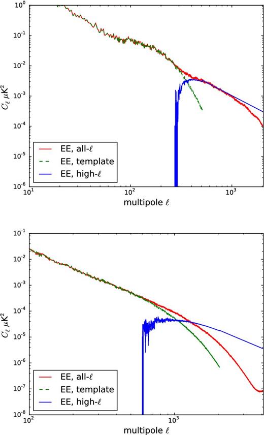
Synchrotron (top) and thermal dust (bottom) templates EE power spectra. The BB spectra is very similar, so it is omitted for clarity. The green curve corresponds to the original template. The blue curve is the high-ℓ extension, where the slope is extended to higher multipoles by a power-law fit. The red curve corresponds to the power spectra of the template map including the artificial high-ℓ features. Note that the red curve includes a 5 arcmin beam smoothing, whereas the blue curve is an extrapolation without smoothing.
For the EE power spectrum, we fitted for the slope in the multipole interval 10 ≤ ℓ ≤ 120 and obtained a value of −1.7 ± 0.04; for the BB power spectrum, we fitted for it in the interval 4 ≤ ℓ ≤ 40 and obtained a flatter slope of −1.4 ± 0.05. We obtained power spectra for the high-ℓ features as the difference between the original spectrum and its extrapolation computed using the best-fitting slope. This procedure creates a smooth high-ℓ power spectrum, shown in blue in Fig. 2 (top). After this, we create a realization map with the artificial high-ℓ power spectrum, using synfast and using a Gaussian beam appropriate for the resolution of the simulation.
We finally multiply the resulting random map by a normalized version of the original template map. This reproduces the anisotropy of the foreground map (a Galactic plane mask in a sense), where regions in the Galactic plane are typically much brighter than at high latitudes. The high-ℓ random map is finally added to the original template, but multiplied by an amplitude chosen to give a continuous power spectrum at multipoles corresponding to the original beam. The power spectrum of the resulting map (for a 5 arcmin final resolution) is shown in Fig. 2 (top) in red.
We follow the same procedure for the dust template. Fitting for the EE and BB slope in the range 60 ≤ ℓ ≤ 600 yields −2.36 ± 0.005 and −2.16 ± 0.007, respectively. Fig. 2 (bottom) shows the EE power spectra for the dust template, for a final resolution of 5 arcmin. The colour code is the same as in Fig. 2 (top). The slopes of the high-ℓ power spectrum, the beam and the amplitude of the high-ℓ maps are free parameters of the model and can be chosen to give different small-scale features, as needed for the simulation.
2.3 Baseline foreground model
The best-fitting values of Planck Collaboration X (2015) are Td = 21 K and a spatially varying dust spectral index with average value 〈βdust〉 = 1.53 over the sky. For the synchrotron component Planck Collaboration X (2015) uses a template spectrum obtained with the galprop code (Orlando & Strong 2013) instead of a power-law model; the slope of the spectrum between ∼19 and ∼97 GHz corresponds to a βsyn ∼ 3.10. For our baseline model we use spatially constant parameters derived by the Planck Collaboration X (2015) analysis: Td = 21 K, βdust = 1.53 and βsyn = 3.10.
2.4 Spatially varying spectral indices
In order to add complexity to the models, we also considered using spatially varying spectral index maps for both dust and synchrotron emission. For thermal dust, we started from the map of best-fitting spectral indices calculated using the temperature Planck maps from commander in Planck Collaboration X (2015). This map has a resolution of 7.5 arcmin FWHM but it is very noisy. We therefore smoothed it to 3°. The final map of βdust of our model is shown in the top panel of Fig. 3. For our test model, we do not consider spatially varying Td, since there is a degeneracy between βdust and Td. With no ∼THz data, it is very difficult to constrain both at the same time, so we only consider spatially varying βdust, which has more effect on the spectral law in the frequency range we consider.

For synchrotron, we use the map of spectral indices by Giardino et al. (2002). This map was derived using the full-sky map of synchrotron emission at 408 MHz from Haslam et al. (1982), the Northern hemisphere map at 1420 MHz from Reich & Reich (1986) and the Southern hemisphere map at 2326 MHz from Jonas, Baart & Nicolson (1998). The Giardino et al. (2002) map has a resolution of 10°.
One possible problem with the Giardino et al. (2002) map is that it was derived at radio frequencies, where the synchrotron spectral index is typically flatter. We corrected for this effect by computing the expected steepening between ∼490–2120 MHz and 20–30 GHz using the same galprop template used in the Planck analysis and applying it to the Giardino et al. (2002) map. The result is shown in the bottom panel of Fig. 3; the steepening applied is Δβsyn = 0.13. The mean and standard deviation of this map are 2.9 and 0.1, respectively.
2.5 Curved synchrotron spectral index and multiple thermal dust components
2.6 Additional polarized components: Anomalous Microwave Emission (AME)
There is evidence that AME due to spinning dust is polarized, with a polarization fraction of few per cent (Dickinson, Peel & Vidal 2011; Génova-Santos et al. 2015). We consider the polarization intensity of the AME as an additional feature to simulate observations by future experiments with a better accuracy.
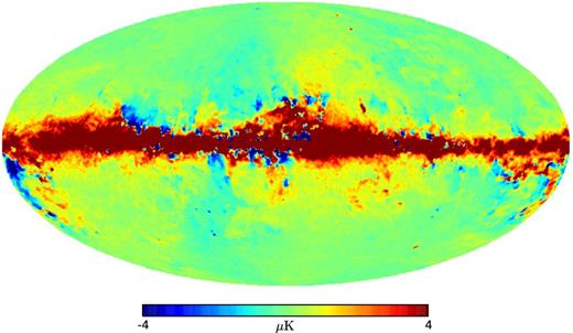
Template map of Q AME component, as derived from the total intensity AME and the thermal dust polarization maps from Planck Collaboration X (2015). This map has 1° resolution, a reference frequency of 23 GHz and assumed a polarization fraction of 0.01.
2.6.1 Adding dust-correlated high-ℓ features to the AME maps
Similarly to what done for the synchrotron and thermal dust components in Section 2.2.1, the AME polarization maps can be upgraded in resolution by adding high-ℓ features. However, in this case we want the high-ℓ thermal dust and AME maps to exhibit the same level of correlation measured at low resolution. We therefore developed a special procedure for this case, that generates both dust and AME high-ℓ correlated random maps at the same time.
We followed the procedure described in Brown & Battye (2011), which uses as input the spectra and cross-spectra of the set of correlated maps (in our case, dust E and B, and AME E and B). This information is used to generate four correlated aℓm fields, which are finally transformed to Q and U with the healpixalm2map function. Extending what is described in Section 2.2.1, the spectra and cross-spectra for the high-ℓ maps are constructed by extrapolating those of the dust and AME templates to higher multipoles. The last step of our procedure, the modulation of the random high-ℓ maps with a mask enhancing the Galactic plane, is unchanged.
3 SIMULATED OBSERVATIONS OF CMB POLARIZATION EXPERIMENTS
3.1 Simulating the instrumental response
To simulate the observation of the microwave sky in polarization by a given experiment, we need to know the frequency bands of observation and, for each of the bands, the point spread function and the noise level. Each of these properties can be simulated with different level of complexity, specified by the user, as detailed in the following.
The effect of the instrumental resolution is simulated by convolving the maps with a Gaussian beam of specified FWHM.
The noise can be modelled either as a uniform white noise, described by a unique rms value over all the sky, or as an anisotropic white noise specifying a map of rms varying in the sky. For Planck, we model this using the 3 × 3 noise covariance per pixel containing the Stokes parameter covariance elements TT, QQ, UU, TQ, TU and QU. In this case, for each pixel, a Cholesky decomposition is performed over the covariance matrix; the diagonal elements of the decomposition finally yield the standard deviations per pixel for T, Q and U, respectively.
3.2 Simulation procedure
Once the experiment is specified, by means of a set of frequencies, resolution and noise, the simulation procedure is the following.
A CMB map is generated using synfast, up to a resolution equal to θ*, which should be at least equal to the smallest instrumental beam of the experiment.
High-ℓ features are optionally added to the synchrotron, dust and/or AME templates up to a resolution θ* (if θ* is smaller than the intrinsic resolution of the template).
The CMB map and foreground templates are scaled in intensity according to the frequency behaviour to each frequency band, added together and smoothed to match the resolution appropriate for that channel.
A noise map is generated and added to the frequency band for each channel to obtain the simulated frequency map.
The outputs are the frequency maps, but also the component maps at all required frequencies. Some of the components can be easily deactivated to obtain noise-only, signal-only, foreground-only or CMB-only simulations, for example for Monte Carlo purposes.
4 COMPARISON WITH DATA FROM PLANCK AND WMAP
4.1 Foreground model
For the comparisons shown in this section, we used the baseline foreground model described in Section 2.3. This includes synchrotron and thermal dust with fixed spectral indices in the sky. We do not include the polarized AME component, that was not detected by Planck due to its weakness compared to the noise levels (Planck Collaboration X 2015).
4.2 Data maps
We compared the output of our model with Planck sky observations in polarization at 30, 44, 70 and 353 GHz, complemented by the WMAPW band at 94 GHz and K band at 23 GHz. In the following, we carried out the comparison between model and data smoothing to a 1° common resolution, which is the resolution of our synchrotron template. Such resolution is also good for display purposes because it reduces the noise and allows an easier visual inspection of the foregrounds morphology.
The Planck frequency maps have been corrected for the polarization leakage due to bandpass mismatch with the correction maps available on the Planck Legacy Archive. The WMAP maps have been downloaded from the LAMBDA-WMAP archive.3
4.3 Comparison with foregrounds only
We first compared the data with a model of the sky including only the foregrounds (with no high-ℓ features) and without CMB and noise. In this way, we only compare the deterministic components of the model, without any random realization. The true Planck and WMAP frequency responses have been used to create the model sky as described in Section 3.
Fig. 5 shows a pixel-by-pixel comparison of true versus model Q and U maps. We show only the pixels inside the Galactic plane (|b| ≤ 20°) for Nside = 64 to reduce the effect of noise and CMB. Fig. 6 shows the maps in pseudo-colour scale, for six frequencies and in Q and U intensity. The modelled foregrounds and the observed sky have the same colour scale. As expected, the agreement is very good for the foreground-dominated frequencies. At 70 and 94 GHz the agreement is less good, because CMB and noise become important. The direct comparison of the maps shows that the foreground model is quite good once the noise is reduced (by means of degrading to Nside = 32). The U intensity of the 94 GHz band is noisy, which makes the comparison difficult.
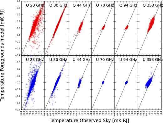
Scatter plot inside the Galactic plane |b| ≤ 20°. The Nside is 64. The top row corresponds to Q intensity, and the bottom row to U intensity. The black line represents the perfect one-to-one match. Both the templates and the observed sky were smoothed to a common 1° resolution.
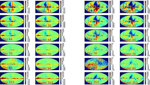
Maps comparison between the observed sky and the foreground model. Left: maps for Q intensity. Right: maps for U intensity. The rows are six bands, the left-hand column corresponds to the observed sky and the right one to our foregrounds model. The units are μKA. The maps are smoothed to a common 1° resolution and degraded to Nside = 32 to suppress the noise for display purposes.
4.4 Including the contribution from noise and CMB
For the comparisons presented in this section, we included noise and a CMB realization, which are present in the sky observations, in order to assess the match of the model when all components are included. In this case we only consider the power spectra, since the different CMB and noise realizations do not allow a morphological comparison.
The CMB map has been generated starting from the best-fitting model of Planck (including polarization information, Planck Collaboration XIII (2015)) and with tensor-to-scalar ratio r = 0.1.
In this case, we consider the 30, 44, 70 and 353 GHz Planck bands and all five of the WMAP bands. The WMAP noise is simulated using the hit counts maps and rms information available from the Lambda website. Planck noise has been simulated using the pixel covariance information. However, this noise is based on the Planck data before applying the leakage correction maps, while the data used for the comparison have the correction applied. As illustrated for 70 GHz in Fig. 7, the bandpass correction subtracts a large fraction of the noise, therefore the noise contribution at small scales is overestimated. For this reason, the comparison that follows is limited to ℓ ≤ 100 where this effect is not significant.
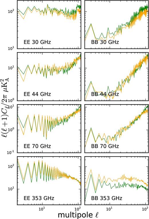
EE (left) and BB (right) full-sky power spectra comparison between the complete model (foregrounds+noise+CMB, in green) and the observed sky (in orange) in four Planck bands, for Nside = 256. The error for the observations is plotted as the orange shaded region. The full-sky maps are smoothed to a common 1° resolution.

EE (left) and BB (right) full-sky power spectra comparison for the five WMAP bands. The error for the observations is plotted as the orange shaded region. The full-sky maps are smoothed to a common 1° resolution. The convention is the same as in Fig. 8.
The agreement between the intermediate frequencies (44 and 70 GHz) benefits from the inclusion of CMB and noise in the comparison. At 70 GHz the CMB polarized intensity is strong, so the match improves. The inclusion of noise is particularly important to reconcile model and data towards ℓ = 100.
4.4.1 Comparison on small patches at high Galactic latitude
As a final assessment of our model, we compare local power spectra to the latest Planck observations in several small sky patches at intermediate and high Galactic latitude. This is particularly useful for ground-based CMB polarization experiments, which target these areas. For example, the BICEP2/KECK array (BICEP2 Collaboration et al. 2014) observes with two bands at 100 and 150 GHz. They target a high Galactic latitude patch visible from the South Pole, with a size of ∼800 deg2. The South Pole Telescope has measured the sub-degree scales lensing BB power spectrum in a southern 100 deg2 patch using two bands (95 and 150 GHz) (Keisler et al. 2015). Another example is the POLARBEAR experiment, in the Atacama desert in Chile, which measured the lensing BB spectrum in three small patches with a total area of 25 deg2 at 150 GHz (The Polarbear Collaboration: Ade et al. 2014). Given the frequency coverage of these experiments, observing around 150 GHz, where the CMB peaks, it is crucial to model correctly the contamination from polarized thermal dust emission.
For our comparison, we followed a similar procedure to the one described in Planck Collaboration XXX (2016) for assessing the contamination by thermal dust. We produced disc-shaped masks with a radius of 11| $_{.}^{\circ}$|3 (400 deg2). Each patch is located on the centre of a pixel of an Nside = 8 map and we considered patches whose centre has a latitude of |b| > 45°. This leaves 48 circular patches. We also added another mask that selects the region targeted by BICEP2/KECK. The masks are apodized by smoothing with a 2° FWHM beam.
We used the same maps assessed in Fig. 8 (Nside = 256, 1° FWHM resolution, modelled as foregrounds + noise + CMB). On each small patch, we calculated the pseudo-Cℓ for both our model and the Planck observations at 353 GHz, in order to compare the thermal dust polarization intensity. Then, we corrected for the effect of masking with a pseudo-Cℓ approach (e.g. Brown, Castro & Taylor 2005). Following Planck Collaboration XXX (2016), we fitted for the power law |$D^{XX}_{\ell }=A^{XX}(\ell /80)^{\alpha _{XX}+2}$|, where XX is either EE or BB, using the same fitting method described in Section 2.2.1 over a range of multipoles ℓ = 40–100.
To assess the match, we plot the fitted AXX and αXX from the model and from Planck 353 GHz observations in Fig. 10. The crosses represent each one of the disc-shaped patches, while the star represents the BICEP2 field for either EE or BB. The agreement is better on the foreground amplitude AXX than on the slope αXX, our model being generally a bit steeper than the Planck 353 GHz channel. For the patches having lowest signal, the mismatch is mostly due to errors in modelling the noise, as detailed in Fig. 7 . For the signal-dominated patches, the mismatch is more likely due to foreground modelling. The Planckcommander analysis that produced the templates was optimized for the full-sky rather than a small sky patch. As a consequence, the match on individual 400 deg2 sky areas may vary, but there is good agreement when considering a sample of sky patches.
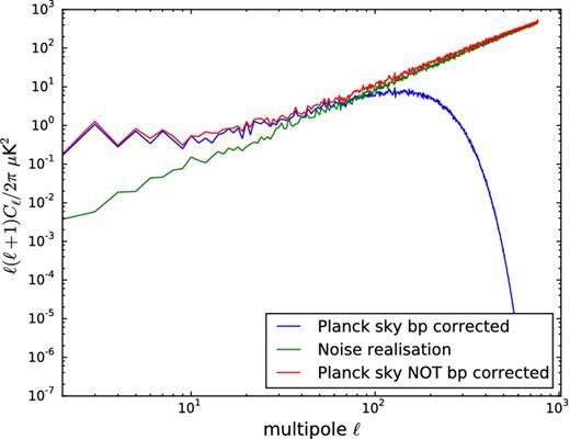
Full-sky BB power spectra with Nside = 256 for both the Planck sky maps at 70 GHz before (red) and after (blue) bandpass leakage correction. A noise realization (green) agrees well at high-ℓ, but since the bandpass leakage correction affects the noise, there is no agreement anymore with the noise level.
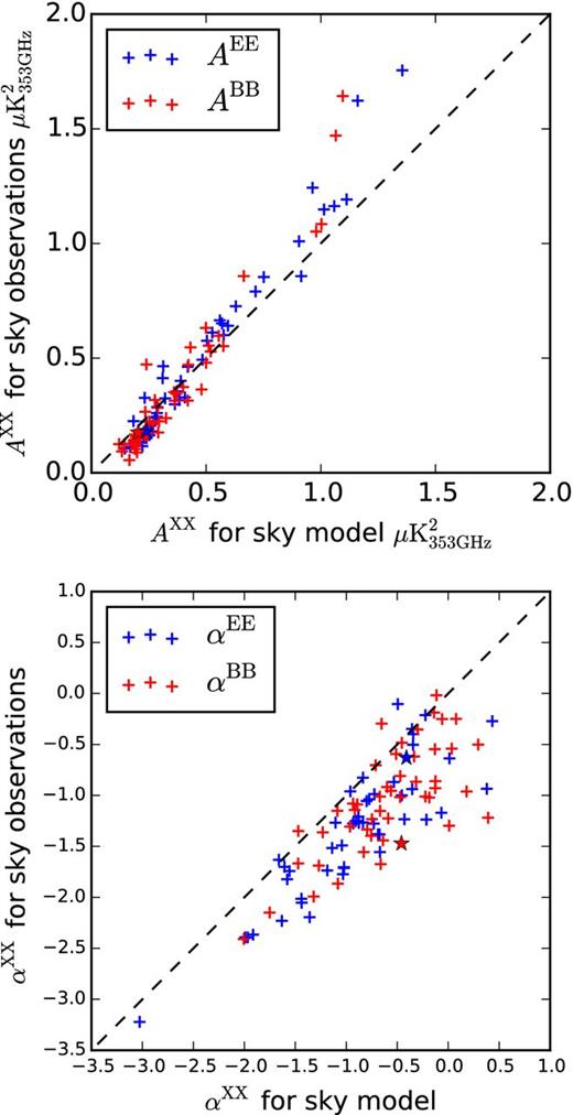
Correlation of the fitted power-law between our model and Planck 353 GHz observations for several intermediate and high latitude small patches. Top, correlation for the value of the amplitude AXX at ℓ = 80. The stars correspond to the BICEP2 field. Bottom, correlation between the values of the power-law slope αXX.
4.5 Optimal spectral index test
In the previous tests, we used the best-fitting values for the spectral indices βsyn = 3.10 and βdust = 1.53, according to Planck Collaboration X (2015). We might wonder if this is the optimal choice. Here, we explore the possibility that changing the spectral index of synchrotron and/or dust may improve the match. This analysis will also provide indications of what is a reasonable range within which to vary the synchrotron and dust spectral indices, for example for Monte Carlo purposes, while preserving good agreement with the data.
We mapped the χ2 values for a grid of (βdust, βsyn) parameters and for both the 70 and 44 GHz bands. We could not use the Planck 30 and 353 GHz because those are the frequencies at which the synchrotron and dust templates are normalized, therefore are unaffected by changing the spectral indices. Also, we did not consider the WMAP channels because of their higher noise levels. We finally obtained a joint likelihood for the 44 and 70 GHz channels as exp (−χ2/2), where |$\chi ^2=\chi ^2_{44\, \rm GHz}+\chi ^2_{70\,\rm GHz}$|.
In Fig. 11 we show the results for the pixels inside a b = ±20° Galactic strip. The left-hand panel corresponds to the Q maps, the right one to the U maps. The black curve corresponds to the 1σ confidence interval in the βdust–βsyn space considered. Note that we assume a prior on the range of values these indices can take. The probability distribution is flatter in U (and therefore the 1σ contour is wider) because the U maps have weaker foreground emission, as can be seen in Fig. 6.
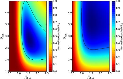
Normalized probability for βdust and βsyn obtained by adding the χ2 values for two Planck bands: 44+70 GHz. In this case, the pixels inside a Galactic latitude b ± 20° are used. The black curve represents the 1σ confidence interval. The left-hand panel shows the constraints given by Q maps, and the right one those given by U maps.
The best-fitting values for the 1D marginalized probability of each parameter and its 1σ confidence interval, adding both bands and both polarizations (44 + 70 GHz and Q + U), are |$\beta _{\rm syn}=3.4^{+0.7}_{-0.5}$| and |$\beta _{\rm dust}=1.6^{+0.5}_{-0.2}$| for the pixels inside the Galactic plane strip, and |$\beta _{\rm dust}=1.6^{+0.6}_{-0.3}$| and |$\beta _{\rm syn} = 3.4 ^{+0.9}_{-0.6}$| when we consider the full-sky. The reason why we obtain relatively weak constraints is because we could only use data at central frequencies, where foregrounds are not so strong and the two spectral indices are more degenerate. A test of the model with much lower (higher) frequency would give a much stronger constraint of the synchrotron (dust) spectral index.
5 FORECAST AND MONTE CARLO CAPABILITIES
To illustrate the simulation capabilities of our sky model we consider the specifications of the Cosmic Origin Explorer (COrE) experiment described in The COrE Collaboration et al. (2011). The instrumental specifications are reported in Table 1. This experiment has 15 frequency bands with frequency ranging from 45 to 795 GHz and resolution of 23–1.3 arcmin. The noise is simulated as Gaussian and uniform, with standard deviation of a few μK per arcminute, as quoted in the table.
Reference values used for simulating COrE observations.
| Band (GHz) | 45 | 75 | 105 | 135 | 165 | 195 | 225 | 255 | 285 | 315 | 375 | 435 | 555 | 675 | 795 |
|---|---|---|---|---|---|---|---|---|---|---|---|---|---|---|---|
| Beam FWHM (arcmin) | 23.3 | 14.0 | 10.0 | 7.8 | 6.4 | 5.4 | 4.7 | 4.1 | 3.7 | 3.3 | 2.8 | 2.4 | 1.9 | 1.6 | 1.3 |
| Noise (μK·arcmin) | 8.61 | 4.09 | 3.5 | 2.9 | 2.38 | 1.84 | 1.42 | 2.43 | 2.94 | 5.62 | 7.01 | 7.12 | 3.39 | 3.52 | 3.60 |
Fig. 12 shows the forecasted B mode for foregrounds for COrE as obtained with our sky model. The CMB BB power spectra for different tensor-to-scalar ratios are compared with the foreground power at three COrE frequencies: 45, 105 and 315 GHz. The foreground power spectra have been computed with the WMAP polarization mask (excluding ∼37 per cent of the sky); it has been corrected for again using the pseudo-Cℓ approach of Brown et al. (2005). Although this figure is qualitatively similar to other forecasts in the literature (e.g. The COrE Collaboration et al. 2011), the fact that our model is based on actual polarization observations ensures a better match with the real sky and therefore improved forecast capabilities.
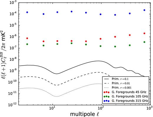
Forecast for primordial BB modes detectability. The black curves show primordial |$C_{\ell }^{BB}$| for three values of the tensor-to-scalar ratio. We also show the BB power spectra for polarized foregrounds for three frequencies: 45, 105 and 315 GHz. The foreground maps were masked with the WMAP polarization data analysis mask and deconvolved from pseudo-Cℓ following Brown et al. (2005).
In Fig. 13 we show the Q intensity on a 30° × 30° sky patch located at l = 180°, b = 30° and exhibiting intermediate foreground contamination. The top-left panel shows a CMB realization with 4 arcmin resolution. The remaining panels show the simulated COrE observations in this region at 45 GHz, dominated by synchrotron emission, 105 GHz, dominated by CMB emission and 315 GHz, dominated by thermal dust emission. The resolution in each panel is different and corresponds to the COrE resolution quoted in Table 1. The features of the foreground components are easily viewed. On the smallest scales, the foregrounds structures are those generated with the procedure described in Section 2.2.1, which allows overcoming the limits imposed by the intrinsic resolution of the templates (1° for synchrotron and 10 arcmin for thermal dust).
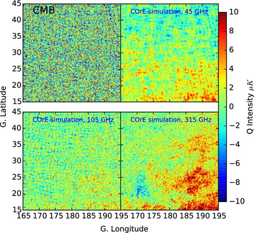
Zoomed-in region of intermediate foreground contaminations in a simulation of COrE observations. The maps are patches of Q intensity, 30° × 30°, centred at l = 180°, b = +30°. The top-left panel shows a CMB realization (in thermodynamic units), and the remaining panels show the simulated observations for three frequencies: 45 GHz (dominated by synchrotron emission), 105 GHz (dominated by CMB) and 315 GHz (dominated by thermal dust emission). These panels have antenna units.
As mentioned, a valuable feature of our sky model is the capability to randomize to a certain degree the polarized foreground components, for example for Monte Carlo purposes. This can be particularly useful to produce simulations that reflect our uncertainties on the polarization of the foregrounds. The randomization method exploits the same procedure described in Section 2.2.1 to upgrade the resolution of the templates. By changing the parameters describing the power spectrum of the high-ℓ map (such as the slope and normalization), it is possible to obtain fainter/stronger foreground contamination at intermediate and small scales. Moreover, by changing the seed of the random realization, it is possible to obtain independent patterns for the same configuration. This is illustrated in Fig. 14, where we show the Q intensity for the synchrotron emission in a 5° × 5° patch of the sky centred in the same coordinates as Fig. 13. The top panels show the original synchrotron emission template at 1° resolution on the left and a high-resolution (5 arcmin) one on the right. The bottom panels show two alternative versions of the top-right panel: a different realization with the same power spectrum on the left and the same random realization with steeper power spectrum (and therefore fainter foreground features) on the right.
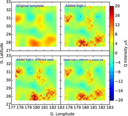
Illustration of the foregrounds randomization capabilities of the code on a 5° × 5° sky patch centred at l = 180°, b = 30°. The top-left panel shows the original Q synchrotron template, which has a FWHM of 1°; the top-right panel shows the same template upgraded in resolution to 5 arcmin by adding high-ℓ features. The bottom-left panel shows the same as the top right, but with a different random realization. The bottom-right panel shows the same as the top-right one, but with a steeper power spectrum at high multipoles (and therefore fainter foreground features).
6 CONCLUSIONS
We have constructed and validated a new model of the microwave sky in polarization, based on the most recent results from the Planck experiment (Planck Collaboration VI 2015). Our model features multiple choices for the frequency dependence of the polarized synchrotron and dust foregrounds of increasing complexity. The templates, based on the Planck observations, are upgraded in resolution by means of a random map modulated by the large-scale foreground emission. This allows simulating experiments with higher resolution than Planck. At the same time, it allows randomizing over the small-scale foreground features, for example in a Monte Carlo approach. We also include curvature in the synchrotron spectral law, and the capability to model an arbitrary number of modified black bodies for the thermal dust law. Finally, we include the choice of a polarized AME emission template, constructed from the thermal dust polarization angles and from the AME total intensity template provided by Planck.
We demonstrated that our baseline model (power-law synchrotron with fixed spectral index βsyn = 3.10, modified blackbody thermal dust with fixed temperature Td = 21 K and spectral index βdust = 1.53) gives a very good match with both WMAP and Planck data. We also found good agreement between the dust model and the data on small high-latitude regions, typically targeted by ground-based experiments. When changing the parameters of the model, βsyn = 2.9–4.2 and βdust = 1.4–2.1 also provide a good fit to the data.
We finally showed the capabilities of our model for forecast and Monte Carlo purposes by simulating data for the COrE experiment. Our easy to use python package, which we make fully available,4 will be a useful tool for the CMB polarization community.
CHC acknowledges the funding from Becas Chile/CONICYT. AB and MLB acknowledge support from the European Research Council under the EC FP7 grant number 280127. MLB also acknowledges support from an STFC Advanced/Halliday fellowship. We gratefully acknowledge the anonymous referee for useful suggestions that led to the improvement of this paper.
REFERENCES
