


Abstract
We present results from hydrodynamic simulations with forced turbulence at a scale of 50 pc and cooling functions adapted to describe the thermal conditions at four different Galactocentric distances: 8.5, 11, 15, and 18 kpc. These experiments are aimed to study the effects of varying the turbulent velocity vrms on the cold gas mass fraction. With realistic vrms we obtain average one-dimensional cold gas mass fractions which are comparable with the observed values. Our simulations can also lead to an approximately constant cold gas mass fraction for distances ≥11 kpc when considering subsonic perturbations for 15 and 18 kpc. We also find that the average one dimensional cold gas mass fraction and the volumetric cold gas mass fraction do not follow the same radial trends.
1 INTRODUCTION
In our Galaxy the atomic gas is the most massive component of the ISM. In this gas, the radiative cooling and heating processes allow for the presence of the isobaric mode of thermal instability (TI; Field 1965) producing the segregation of gas in two stable phases, known as the warm neutral medium (WNM; T ∼ 600–8000 K) and the cold neutral medium (CNM; T ∼ 20–250 K) which, in the ideal case where TI can freely proceed, co-exist in pressure equilibrium within a range of thermal pressures. It is now well established that in the real ISM the interplay between the TI and other physical ingredients such as turbulence, gravity or magnetic fields plays an important role on the structure of the gas. In fact, considerable amounts of gas with temperatures in the thermal unstable range have been measured in observations as well as in numerical simulations (e.g. Gazol et al. 2001; Heiles 2001; Piontek & Ostriker 2004; Seifried, Schmidt & Niemeyer 2011)
The formation of cold atomic gas has been recognized as an important ingredient for the molecular cloud formation because it is thought to be the first step of this process but also because the properties of the initial atomic gas seem to have important consequences on the structure and on the evolution of the resulting molecular gas. At small scales, in simulations of molecular cloud formation by colliding flows, it has been observed that the formation of a cold atomic cloud and its rapid mass growth induce the gravitational collapse leading to star formation (see e.g. Inoue & Inutsuka 2012; Dobbs et al. 2014, and references therein). A recent observational proof of the association between cold atomic gas and star formation regions is the detection of an increased amount of CNM associated with the Perseus cloud, as revealed by the presence of a higher fraction of absorbing H i and a higher total H i column density relative to the mean local ISM (Stanimirović et al. 2014).
At galactic scales, the available amount of CNM has been proposed by different groups as a major agent in the regulation of star formation activity. Elmegreen & Parravano (1994) and Schaye (2004) explained the sharp edges of the star formation rate (SFR) and the stellar surface density as a consequence of a density threshold determined by the ability to form cold atomic gas. Bonnell, Dobbs & Smith (2013) conclude, from numerical simulations aimed to study the relationship between SFR and cooling in spiral galaxies, that cooling is the primary driver of star formation as it determines the amount of cold gas available for gravitational collapse. On the other hand, Bigiel, Cormier & Schmidt (2014) compare scaling relations between gas and star formation in the outer discs to those obtained for the optical discs of nearby galaxies. In the inner parts, the molecular gas exhibits a strong correlation with the SFR, whereas the atomic gas shows no clear correlation. In contrast, in the outer discs SFR scales with the H i surface density, suggesting that the amount of available H i could be a key parameter regulating star formation in these outer regions.
The thermal balance of the atomic gas in the inner and outer disc of the Galaxy has been studied by Wolfire et al. (2003), who found that, for Galactic radii between 3 and 18 kpc, the thermal equilibrium curve has the same shape as for 8.5 kpc; including a region where the Field's criterion for isobaric TI is satisfied (see Section 2.3). In principle, this implies that for all these radii the atomic gas could be segregated in two thermally stable phases if thermal pressure lies within the pressure range in which the CNM and the WNM can co-exist. However, when velocity fluctuations drive perturbations in a thermally unstable gas, the TI development occurs only when the cooling time τcool is short enough compared to the dynamical time τd, which in turn depends on the perturbation scale (see Section 2.3). At 8.5 kpc this condition is fulfilled by the WNM in thermal equilibrium for scales larger than approximately 20 pc, while for thermally unstable gas a minimal perturbation scale of few parsecs is needed (see e.g. Audit & Hennebelle 2005; Gazol, Vázquez-Semadeni & Kim 2005; Saury et al. 2014). In fact, the statistical properties of a turbulent thermally bi-stable gas in physical conditions similar to those of the solar neighbourhood have been extensively studied through numerical simulations (Gazol et al. 2005; Piontek & Ostriker 2005; Brandenburg, Korpi & Mee 2007; Hennebelle & Audit 2007; Gazol, Luis & Kim 2009; Audit & Hennebelle 2010; Gazol & Kim 2010; Seifried et al. 2011; Gazol & Kim 2013; Gazol 2014; Saury et al. 2014).
The existence of CNM at large Galactocentric distances in the Milky Way has been proved both indirectly by the presence of star formation regions up to a radius Rg ∼ 17–20 kpc (e.g. Snell, Carpenter & Heyer 2002), and directly by the detection of H i absorption towards continuum background sources in the outermost spiral arms, indicating a widespread presence of cool H i between Galactocentric radii of 12 and 25 kpc (Strasser et al. 2007).
A puzzling observational result concerning the distribution of CNM in the Galactic Mid-plane has been obtained by Dickey et al. (2009), who studied the temperature of the H i in the outer disc of the Milky Way. They used data from three 21 cm Galactic Plane surveys (the Canadian Galactic Plane, Survey Taylor et al. 2003; the Southern Galactic Plane Survey, McClure-Griffiths et al. 2005; and the VLA Galactic Plane Survey, Stil et al. 2006) to find that the ratio of the emission to the absorption (resulting from averaging over annuli of constant Rg), which gives the mean spin temperature of the gas 〈Tsp〉, stays nearly constant with radius at ∼400 K from ∼12 to ∼25 kpc, suggesting that the mixture of CNM and WNM, measured by 〈Tsp〉 remains approximately constant for a wide range of physical conditions. Assuming that the CNM has a unique temperature between 40 and 100 K, and that the gas is well segregated in two phases, they estimate a CNM mass fraction ϕc ∼ 10–25 per cent at Rg = 12–25 kpc. This method has been recently tested by Kim, Ostriker & Kim (2014) using synthetic 21 cm observations to compare the cold gas mass fraction determined by using 〈Tsp〉 with the cold gas mass fraction directly measured from their simulations. For this, they use three-dimensional hydrodynamic simulations of multiphase gas modelling a local patch of the Galactic disc and including Galactic differential rotation, external gravity from stars and dark matter, gaseous self-gravity, interstellar cooling and heating, and feedback from star formation (Kim, Ostriker & Kim 2013). They find that the spin temperature represents a good estimator of the cold gas mass fraction when the cold gas temperature is well constrained and the spin temperature is ≤400 K.
An observational result similar to the one described above has been obtained by Pineda et al. (2013). They combine maps of the Galactic Observations of the Herschel Terahertz C+ (GOTC+) project, which survey the [C ii] 158 μm line over the entire Galactic disc, with other maps of H i, 12CO, and 13CO to separate the different phases of the ISM and study their properties and distribution in the Galactic plane. In order to determine the azimuthally averaged distribution of CNM they assume that this gas is at a uniform temperature of 100 K and consider that spaxels with H i emission but neither [C ii] nor 12CO emission contain only WNM. They find that at Rg = 8.5 kpc, the cold gas mass fraction is in good agreement with the local value of 0.4 derived by Heiles & Troland (2003) whereas at larger Galactocentric distances this fraction decreases to only 0.1–0.2, showing little variation with Rg.
The aim of this work is to test to what extent differences in turbulent velocity dispersion, vrms, of the atomic gas can play an important role on keeping an approximately constant CNM mass fraction at Galactocentric distances larger than 8.5 kpc as indicated by the observations described above. We are motivated to study the relation between vrms and the cold mass fraction for the following reasons. On one hand, previous numerical work shows that in the presence of forced turbulence the fraction of cold gas decreases with vrms (Audit & Hennebelle 2005; Gazol 2014; Saury et al. 2014). On the other hand, observational works report a radial decrease in the total (turbulent + thermal) H i velocity dispersion even beyond the optical radius, in nearby external galaxies (Petric & Rupen 2007; Tamburro et al. 2009; Ianjamasimanana et al. 2015). Although the reported values of the velocity dispersion in the H i gas lie in a surprisingly narrow range between ∼3 and 20 km s−1 for a wide range of physical conditions (Dickey, Hanson & Helou 1990; Heiles & Troland 2003; Haud & Kalberla 2007; Tamburro et al. 2009; Ianjamasimanana et al. 2015), the ability of the gas to segregate and form cold gas is sensitive to the velocity even within this range.
To study the effect of variations in vrms at different Galactocentric distances, we use hydrodynamic simulations with driven turbulence, cooling functions and initial conditions adapted to different values of Rg.
The paper is organized as follows. In the next section we describe the model, in particular the cooling functions and the initial conditions. Then in Section 3 we present our results concerning some global properties of the simulations and the behaviour of the cold mass gas fraction. These results are discussed in Section 4. Finally, in Section 5 we present a summary along with our conclusions.
2 THE MODEL
We analyse three-dimensional hydrodynamic simulations similar to those discussed in Gazol & Kim (2010), which use a periodic box with 100 pc per side and solenoidal Fourier forcing at a fixed wavenumber corresponding to scales of 50 pc. This scale choice allows us to study a simple configuration in which the effects of the disc rotation and stratification, as well as localized feedback sources, can be neglected. In doing so, we are able to test the effects of varying vrms. At the same time, with this scale we can attain an acceptable resolution of ∼0.2 pc at the moderate number of cells of 5123, with which we can explore different vrms values for each Rg.
The use of Fourier space forcing, which implies a continuous and non-localized energy injection, can introduce some artificial effects (see Gazol & Kim 2013). However, with this kind of driving we are able to test the effects of varying vrms with no need of the free parameters associated with other kind of energy injection.
In order to take into account the different physical conditions corresponding to different Rg we consider different cooling functions and different initial conditions.
2.1 Cooling and heating
The cooling functions are piece-wise power law fits to the thermal equilibrium curves (p/k versus n) presented in Wolfire et al. (2003) for Rg = 8.5, 11, 15 and 18 kpc. The cooling rate have the form |$\Lambda =\Lambda _iT^{\beta _i}$|. For the fits we assume, as a first approximation, that for each radius the heating rate has a constant value |$\Gamma _{\rm R_{\rm g}}$| which is also determined from Wolfire et al. (2003) results. For each value of Rg we use their expression for the photoelectric heating rate per unit volume nΓpe as a function of the particle density n, the heating efficiency ϵ, the FUV radiation field G0, and the electron density ne (equations 19 and 20 in Wolfire et al. 2003) to compute Γpe using the scaled value of the FUV field. For ϵ, we compute the arithmetic mean between its values for ne corresponding to the average density and temperature of the warm and cold phase, whose values are given in their table 3. The resulting densities (nCNM and nWNM) and temperatures (TCNM and TWNM) defining the thermally unstable range at each Rg as well as the values of |$\Gamma _{\rm R_{\rm g}}$| are given in Table 1.
Cooling and heating properties.
| Rg | |$\Gamma _{\rm R_{\rm g}}$| | TCNM | TWNM | nCNM | nWNM |
|---|---|---|---|---|---|
| kpc | 10−27erg cm3s−1 | K | K | cm−3 | cm−3 |
| 8.5 | 22.4 | 279 | 5593 | 4.8 | 0.86 |
| 11 | 9.56 | 272 | 5628 | 3.5 | 0.43 |
| 15 | 2.09 | 245 | 6087 | 2.0 | 0.23 |
| 18 | 1.27 | 198 | 6778 | 1.4 | 0.18 |
| Rg | |$\Gamma _{\rm R_{\rm g}}$| | TCNM | TWNM | nCNM | nWNM |
|---|---|---|---|---|---|
| kpc | 10−27erg cm3s−1 | K | K | cm−3 | cm−3 |
| 8.5 | 22.4 | 279 | 5593 | 4.8 | 0.86 |
| 11 | 9.56 | 272 | 5628 | 3.5 | 0.43 |
| 15 | 2.09 | 245 | 6087 | 2.0 | 0.23 |
| 18 | 1.27 | 198 | 6778 | 1.4 | 0.18 |
2.2 Initial conditions
The gas in our simulations is initially at rest and has uniform density n0 and temperature T0 with thermal equilibrium values in the thermally unstable regime. The initial density values are computed by assuming that at Rg = 8.5 kpc n = 2 cm−3 and using the radial volume density exponential distribution for H i given by Kalberla & Kerp (2009), which includes the effects of the asymmetry observed for Rg > 15 kpc and attributed to the warp.
Note that n0 at 8.5 kpc is larger than the value given by Kalberla & Kerp (2009), 0.9 cm−3 and than the density estimated by combining the value of the mean density (weighted by volume filling factor) in the Solar Neighbourhood given by Dickey & Lockman (1990) |$\bar{n}=0.57$| cm−3 and the H i filling factor presented by Kalberla & Kerp (2009, ∼0.42), which is |$\tilde{n}=1.36$| cm−3. Our choice is due to the fact that a gas with |$\tilde{n}$| in thermal equilibrium according to our cooling function is very close the warm stable branch.
The initial density values and the corresponding thermal equilibrium temperatures are listed in Table 2 (second and third columns). Note that the density value for 18 kpc is larger than the value given by the exponential distribution that we use for 11 and 15 kpc. This is because, as we explain in Section 2.3, smaller values do not lead to the development of TI at the scales that we consider.
Initial conditions.
| Rg | n0 | T0 | τcool0 | T50 | n0c | n0w | fc0 | τ0 |
|---|---|---|---|---|---|---|---|---|
| kpc | cm−3 | K | 106 yr | K | cm−3 | cm−3 | – | 106 yr |
| 8.5 | 2.0 | 1500 | 0.44 | 12,641 | 27.05 | 0.35 | 0.84 | 4.23 |
| 11 | 0.904 | 2052 | 1.41 | 7166 | 20.13 | 0.24 | 0.74 | 7.91 |
| 15 | 0.479 | 1817 | 5.71 | 2600 | 13.97 | 0.11 | 0.78 | 22.2 |
| 18 | 0.4 | 1247 | 10.42 | 1355 | 8.46 | 0.06 | 0.86 | 29.1 |
2.3 Instability conditions
In Table 2 we show the cooling time, computed with equation (1) for the initial conditions τcool0 (fourth column) and the temperature at which τs = τcool0 for perturbations with λ = 50 pc, T50 (fifth column). As expected from the values of |$\Gamma _{\rm R_{\rm g}}$|, the cooling time for the initial condition increases by more than a factor of 20 when we move from 8.5 to 18 kpc. One can also see that our initial conditions satisfy T0 < T50. In fact, we choose to use a larger n0 at 18 kpc (see Section 2.2) in order to satisfy this condition.
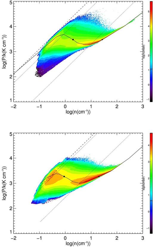
In Fig. 1 we illustrate, for Rg = 11, 15, and 18 kpc, the position of the corresponding initial condition on the thermal equilibrium curve as well as contours of lcrit, which is the critical length at which τs = τcool. For each value of Rg, the dashed line is placed at the corresponding value of T50. For Rg = 18 kpc we also include the initial condition determined by the density distribution described in previous section (n = 0.298 cm−3).

Thermal equilibrium curve, colour contours of lcrit and initial conditions for Rg = 11 (top), 15 (middle), and 18 kpc (bottom). The dashed line corresponds to T50, the filled circle is the initial condition, and the filled diamond is at the thermal equilibrium CNM density at the initial pressure. For Rg = 18 kpc, the filled square is the initial condition determined by the exponential density distribution described in Section 2.2.
2.4 Ideal segregation at initial conditions
In the last column of Table 2 we include also the TI growth times, τ0, for gas at the initial conditions that we use and perturbations with a scale of 50 pc. These times have been computed by solving the linear dispersion relation derived by Field (1965) in the absence of thermal conduction and using our cooling functions. Note that in the non-conductive case, as long as criterion (2) is satisfied, density fluctuations which also satisfy the Field's criterion are unstable and for small enough scales the instability growth rate is independent of the scale. In contrast, when thermal conduction is present it stabilises perturbations with scales smaller than the so called Field's length. In our simulations, which do not include a thermal conduction term, the minimal length required for the perturbations to be unstable is established by the numerical resolution. For a discussion on this subject see Gazol et al. (2005). Comparing the values of τ0 for different radii, it is clear that even if fc0 is comparable, the segregation process could not have the same behaviour at large Galactocentric distances. For 15 and 18 kpc, the values of τ0 are close above τcoolp = τcool(1 − βi)/γ, indicating that in these cases our perturbations are small enough to be close to the regime where the growth rate becomes scale independent.
2.5 The possible effects of neglecting the magnetic field
The simulations presented in the next section are purely hydrodynamic, but in the H i gas magnetic pressure is thought to be of the same order of thermal pressure (Heiles & Crutcher 2005) implying that magnetic field could be a major agent in the determination of the structure of this gas in general and thus on the determination of the CNM mass fraction. Early analytical studies by Field (1965) have shown that the effects of a uniform magnetic field on the segregation due to TI depend on the relative direction between the field and the perturbations. In fact, the analysis of converging flows simulations (e.g. Inoue & Inutsuka 2008, 2009; Chen & Ostriker 2014) shows that when the flows are not parallel to the magnetic field, the formation of high density condensations is inhibited. On the other hand, the density distribution resulting from two-dimensional simulations with forced turbulence (Gazol et al. 2009) seems to be rather insensitive to the presence of magnetic fields. Then, it is not clear how the results reported in this work would be affected in the MHD case but the question deserves more attention and we plan to address it in the future.
3 RESULTS
In this section we report results from thirteen simulations with a resolution of 5123 and whose main properties are summarized in Table 3, where <> indicate time averaged values.
Run properties.
| Rg | 〈vrms〉 | |$\langle\bar{p}/k\rangle $| | 〈Tc〉 | 〈Tmax〉 |
|---|---|---|---|---|
| kpc | km s−1 | K cm−3 | K | K |
| 8.5 | 4.72 | 2548 | 167 | 120 |
| 8.5 | 7.84 | 2769 | 164 | 115 |
| 8.5 | 10.10 | 2861 | 165 | 112 |
| 8.5 | 13.83 | 3003 | 165 | 106 |
| 8.5 | 17.43 | 3162 | 166 | 102 |
| 11 | 7.53 | 1531 | 169 | 123 |
| 11 | 13.66 | 1670 | 171 | 119 |
| 11 | 17.11 | 1788 | 170 | 108 |
| 15 | 2.61 | 705 | 139 | 72 |
| 15 | 4.50 | 730 | 138 | 73 |
| 15 | 7.70 | 816 | 148 | 60 |
| 18 | 2.55 | 404 | 128 | 84 |
| 18 | 3.44 | 415 | 124 | 67 |
3.1 General properties
In Fig. 2, we show the evolution of the three-dimensional rms velocity vrms for each simulation. In this figure, where the first striking feature is the long time during which we ran our models, the units of the x-axis correspond to the time unit of our code t0 = 10.8 × 10⁶ yr. The reason why we choose to evolve our simulations for such long times is explained later in this section. From the same figure it can be seen that simulations with vrms ≳ 7 km s−1 reach a stationary state after less than one time unit, whereas those with smaller velocities spend approximately five time units. In the case of simulations with vrms ∼ 5 km s−1 this could be the consequence of motion induced by the TI development, which constitutes a response to pressure fluctuations and typically produces speeds of the order of tenths of km s−1 (Kritsuk & Norman 2002; Brandenburg et al. 2007; Iwasaki & Inutsuka 2014). For larger times the reduced amount of thermally unstable gas could make this effect less notorious, and for simulations with lower values of vrms the smaller amplitude of pressure fluctuations may also play a role in this sense. Time averaged values of vrms are given in Table 3 (second column).
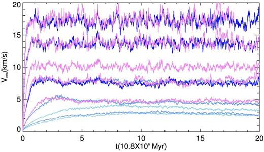
vrms versus time for all models. Violet, dark blue, mid blue, and light blue lines correspond to Rg = 8.5, 11, 15 and 18 kpc, respectively.
Before to proceed with the discussion about the cold gas mass fraction, it is illustrative to look at the log p/k versus log n distribution for different Rg, whose mass weighted version is displayed in Figs 3 and 4. These two-dimensional histograms were computed at random times for simulations with vrms ∼ 7.5–7.9 km s−1. Note that for 18 kpc we do not include this run in Table 3 because it is not discussed in the rest of the paper. For 8.5 and 11 kpc (Fig. 3) the distribution shows a bimodal nature, with considerable masses at the stable branches corresponding to the WNM and the CNM in addition to gas out of thermal equilibrium with approximately isobaric contours at its most concentrated (green or yellow) regions. Note that for 11 kpc the most massive contour (orange) in the warm branch lies between the line placed at the minimum WNM temperature and that placed at T50. For 15 and 18 kpc, (Fig. 4) the distributions are very different. At 15 kpc the gas is segregated, in the sense that the histogram shows two mass peaks, but while the high density gas lies dominantly over the thermal equilibrium curve, the low density gas is concentrated below this curve at unstable temperatures ranging between T50 and the minimal WNM temperature, Tw. For 18 kpc and at this velocity the gas does not segregate and remains concentrated mainly between T50 and Tw. The same kind of behaviour has been reported by Saury et al. (2014) for models with initial thermally unstable gas at pressures higher than those of thermal equilibrium, in cases where the initial density is low enough or the stirring amplitude is high enough.
Two-dimensional mass weighted histograms for simulations with Rg = 8.5 (top) and 11 kpc (bottom). Solid line is the thermal equilibrium curve, dotted lines are the maximum and the minimum temperatures for TI, and dashed line is placed at T50. Circles over the thermal equilibrium density curve are the initial conditions and the thermal equilibrium CNM at the initial pressure.
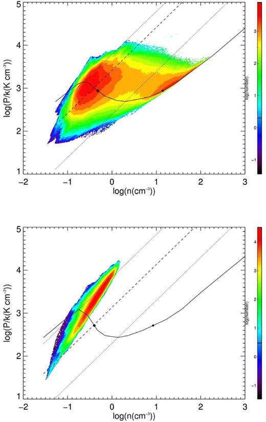
The same as Fig. 3 but for simulations with Rg = 15 (top) and 18 kpc (bottom).
From the values of the initial temperature T0 (Table 2) and vrms (Table 3) it can be seen that in some cases the simulations have vrms smaller than the sound speed at the initial temperature. In those cases we can have a ‘double’ TI development because τd = τs for all the gas with T > T50 (see Section 2.3). By definition this gas does not satisfy the condition τcool < τd in subsonic cases, so that our velocity perturbations, which behave adiabatically, are thermally stable. But this gas satisfies the condition (2), and the density fluctuations generated by the forcing can be thermally unstable if they have temperatures in the unstable range. On the other hand, in cases where vrms > cs and τd = τu, also for the unstable gas with temperatures above T50 τcool > τd and the perturbations are stable, so that gas with temperatures corresponding to the thermally unstable range and T > T50 is stable. When T50 is smaller than the minimal temperature of the WNM, the gas segregates but does not form WNM. This is the behaviour that is observed in the top panel of Fig. 4. To further illustrate it we show in Fig. 5 the mass weighted and the volume weighted temperature histograms resulting from the model with vrms = 7.7 km s−1 at 15 kpc. To improve the statistics we used the outputs corresponding to the last five code time units of this simulation. In both histograms, the peak corresponding to the warm gas lies between T50 (solid line) and the minimal temperature of the WNM according to our cooling functions (dotted line). Only a small fraction of gas reaches this temperature. The cold gas mass peak instead is well below the maximum CNM temperature (dashed black line).
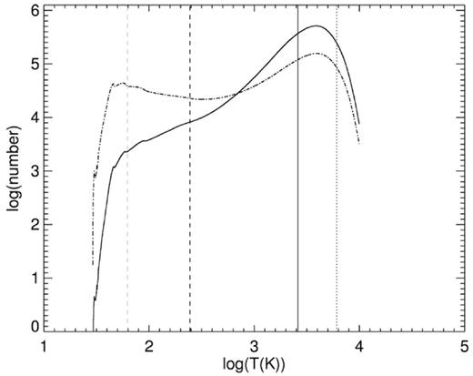
Volume (solid line) and mass (dot–dashed line) weighted temperature histograms for the model with vrms = 7.70 km s−1 at 15 kpc. The vertical lines correspond, from the right, to the minimal WNM temperature (dotted line), T50 (solid line), the thermal equilibrium CNM temperature at the initial pressure (black dashed line), and the minimal WNM temperature (grey dashed line).
Now we address the possible development of the secondary instability. From Figs 1 and 4 it can be seen that, for 15 and 18 kpc, T50 is in the thermally unstable regime. For these distances and small values of vrms it is thus possible to develop a secondary TI due to the thermally unstable density fluctuations generated by the velocity perturbations. As a reference, in Table 4 we show the growth times of TI for perturbations of 50 pc at the unstable transition temperatures |$T_{u_i}$| and the corresponding thermal equilibrium densities for each radius, |$\tau _{u_i}$|. These times have been obtained in the same way as τ0 (see Section 2.3). In order to observe the development of this secondary instability at large distances it is clear that we have to evolve our simulations for more than 15t0. For this reason we choose to run simulations at the four values of Rg for long times (20–25t0).
Thermal instability growth times.
| Rg | Tu1 | τu1 | Tu2 | τu2 | Tu3 | τu3 | Tu4 | τu4 | Tu5 | τu5 |
|---|---|---|---|---|---|---|---|---|---|---|
| kpc | K | t0 | K | t0 | K | t0 | K | t0 | K | t0 |
| 8.5 | 5593.0 | 0.86 | 4500.0 | 0.631 | 1500.0 | 0.344 | 733.33 | 0.757 | 416.67 | 1.64 |
| 11 | 5627.9 | 4.51 | 3833.3 | 1.21 | 1333.3 | 0.529 | 575.00 | 0.857 | – | – |
| 15 | 6087.0 | 17.2 | 4416.7 | 4.33 | 2500.0 | 2.80 | 928.57 | 1.77 | 416.00 | 2.32 |
| 18 | 6777.8 | 19.5 | 5600.0 | 18.3 | 3214.3 | 6.78 | 851.06 | 2.67 | 428.57 | 4.56 |
In Fig. 6 we show the evolution of the CNM mean pressure |$\bar{p_c}$|. It can be seen that |$\bar{p_c}$| increases with vrms, that for Rg ≤ 15 kpc the mean pressure reaches a stationary regime, and that for Rg = 18 kpc the pressure slightly increases with time. It also can be noted that for radii larger than the solar radius the time averaged value of |$\bar{p_c}$| is, for all the simulations, smaller than the initial pressure, while for 8.5 kpc and vrms = 13.5 and 17 km s−1, it is comparable and larger than the initial pressure p0, respectively. This comes from the presence of a large amount of cold high pressure gas, both in thermal equilibrium and out of it. For larger radii and smaller vrms, the cold gas pressure is dominated by gas at p < p0. Note also from the same figure, the large values of |$\bar{p_c}$| at early times for Rg = 15 and 18 kpc.
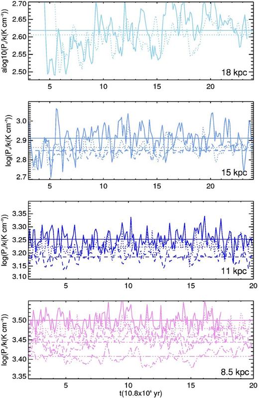
CNM mean pressure as a function of time. The colour code is the same as in Fig. 2. For each radius, the solid line corresponds to the simulation with the largest vrms at this value of Rg. The other lines correspond to decreasing values of vrms in the following order: dotted, dashed, dot–dashed, double-dot–dashed. For each simulation, horizontal lines are placed at the time averaged value (see 3, third column)
3.2 The CNM mass fraction
The simplest criterion to evaluate the mass fraction of cold gas fc is by taking the maximum temperature for the cold stable branch allowed by the cooling function at each radius, Tcnm as the threshold temperature to select cold gas. We call this criterion the cooling curve criterion.
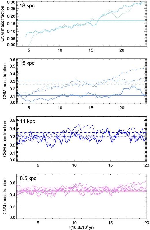
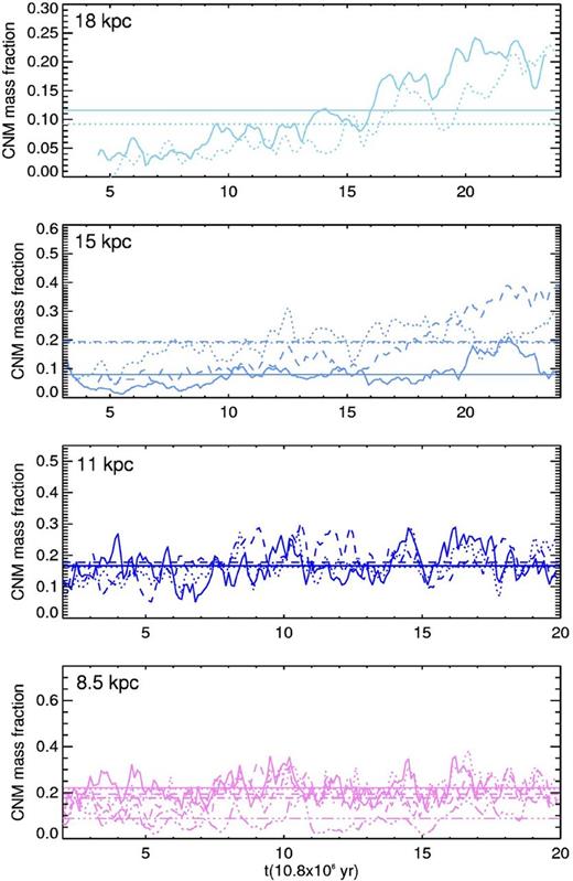
The resulting evolution of fc is shown in Fig. 7 where, when comparing the time averaged values for a fixed radius, it can be seen that fc decreases as vrms increases, which is consistent with previous results (Piontek & Ostriker 2005; Gazol 2014; Saury et al. 2014) from models with cooling functions appropriate to the solar radius. Also, for a fixed velocity fc decreases with radius and in the moderately supersonic case of vrms ∼ 7.5–7.8 km s−1, it goes from ∼0.6 to 0. We can also see that at 8.5 and 11 kpc the volumetric mass fraction is larger than the values reported in the literature, which are ∼40 per cent (Heiles & Troland 2003; Pineda et al. 2013) and ∼10–20 per cent (Dickey et al. 2009; Pineda et al. 2013), respectively, but correspond to the mass fraction along lines of sight. At 15 and 18 kpc, and in spite of the long times during which simulations were ran, the models do not reach a stationary regime. This can be explained by the slow development of the secondary instability described in Section 2.3. Still, for all the simulations we include the time averaged value as a reference. It can be seen that fc tends to decrease with Rg, and that for Rg > 8.5 kpc the dependence with the velocity makes it possible to have approximately the same values of fc for two different radii. However, there is no combination of vrms values giving an approximately constant cold mass fraction for Rg > 8.5 kpc.
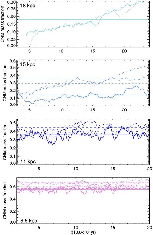
Evolution of the cold gas mass fraction computed with the cooling curve criterion fc. The colour and line codes are the same as in Fig. 6.
Although the previous criterion is physically meaningful, as it reflects the differences among the thermal equilibrium curves at each radius and the real cold gas mass fraction resulting from our simulations, it is not very useful in order to compare with other numerical and observational results. This is because in most cases the shift of Tcnm to lower values is not taken into account and/or a single temperature is assumed for the CNM. Also, exact thermal equilibrium is often assumed when the density, the temperature, and/or the thermal pressure of the atomic gas are calculated from other observed thermodynamic quantities. So, we evaluate the cold gas mass fraction resulting from other four criteria.
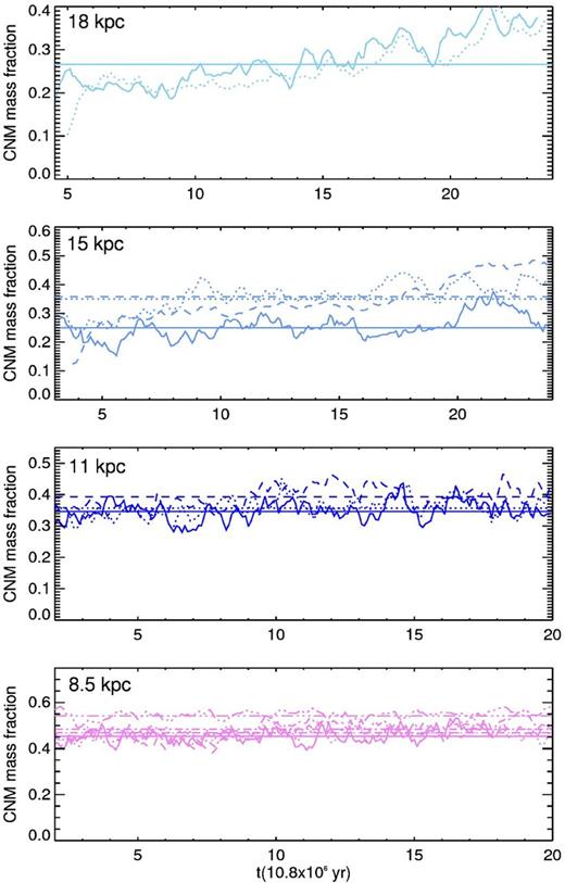
Evolution of fx. The colour and line codes are the same as in Fig. 6.
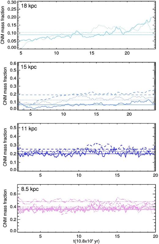
The behaviour of fx with Rg and vrms is not consistent with a scenario where a systematic reduction of vrms with the Galactocentric distance could produce a constant cold mass gas fraction for Rg ≥ 11 kpc. There are three facts which contradict this possibility. First, fx(11 kpc) is smaller than fx(8.5 kpc) for all the values of vrms we explore; secondly, the value of vrms for which fx(11 kpc) is closer to the observed cold mass fraction is the larger one; and thirdly, the velocities for which fx(15 kpc) and fx(18 kpc) are closer to the observed values are only slightly different.
The evolution of fx0, displayed in Fig. 9, shows that for 8.5 kpc the cold mass fraction is slightly above the observed values, but the difference between fx and fx0 increases with Rg indicating a reduction of the two-dimensional cold gas filling factor with the radius. The velocities needed for fx0 to remain approximately constant between ∼0.25 and 0.35 for Rg ≥ 11 kpc are the same as for fx to reproduce the observed trend of the cold gas mass fraction with Rg.
Evolution of fx0. The colour and line codes are the same as in Fig. 6.
3.3 Cold gas selection criteria tests
In this section we study how the fc is related with cold mass fractions evaluated when using different criteria to select the cold gas but which also use the three-dimensional gas distribution.
3.3.1 Pressure criterion
The second criterion we use to define the cold gas and to evaluate the CNM mass fraction consists on finding a threshold temperature, Tp, such that the mean temperature of the cold gas is the thermal equilibrium temperature at the mean pressure, Tpm. This criterion, which we call the pressure criterion, is motivated by the fact that thermal and/or pressure equilibrium is often used to obtain atomic gas properties. From Fig. 10, where the evolution of the ratio Tp/Tcnm is displayed, it can be noted that: (1) Tp is always smaller than Tcnm by a factor of ∼0.4–0.6, which implies threshold temperatures between ∼100 and 170 K. (2) For Rg ≤ 11 kpc, Tp/Tcnm increases with vrms but the opposite is true for larger radii. As expected, Tpm is also smaller than the mean cold gas temperature Tc (see Fig. 11), implying that the mean pressure of the cold gas is higher than the pressure at its mean temperature. Also, the difference between Tpm and Tc is smaller than the difference between Tp and Tcnm. We denote as fp the cold mass fraction obtained using Tp as the maximum temperature of the cold gas. This mass fraction (displayed in Fig. 12) is, for all values of Rg and vrms, smaller than the one obtained by using the temperature indicated by cooling function fc. Note that, with the exception of Fig. 9, in the all figures displaying cold gas fractions, the panel corresponding to each Rg has the same vertical axis; this allows easier comparisons. Interestingly, the values of fp are more consistent with those reported by observations than the values of fc. In particular, at Rg = 8.5 kpc we obtain a mass fraction between 40 and 50 per cent for a large vrms range. We also can account for an approximately constant cold mass fraction between 15 and 25 per cent at larger radii if we consider decreasing values of vrms. Note that for 15 and 18 kpc, the evolution is more spiky than it is when using Tcnm as the threshold temperature. This is a consequence of the fluctuations in the mean pressure (see Fig. 6).
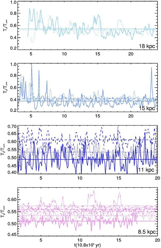
Evolution of the ratio Tp/Tcnm. The colour and line codes are the same as in Fig. 6.
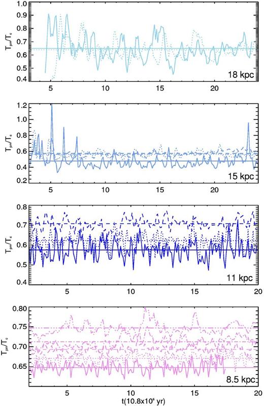
Evolution of the ratio Tmp/Tc. The colour and line codes are the same as in Fig. 6.

Evolution of the cold gas mass fraction computed with the pressure criterion fp. The colour and line codes are the same as in Fig. 6.
3.3.2 The single temperature criterion
It is a common use, in observational as well as in numerical works, to assume that the cold gas is just all the gas with temperatures lower than a fixed value which can be more or less close to Tcnm. So, we evaluate the cold mass fraction obtained by choosing a single maximal temperature for all radii, which is denoted by fT. We take a threshold temperature TT = 180 K, which is slightly larger than the higher values of Tp and smaller than the minimal value of Tcnm (see Table 1, third column). Note also that TT is larger than the time averaged value of the temperature at which the density weighted temperature histogram of cold gas peaks 〈Tmax〉 (see Table 3, last column). When compared with fc, the resulting cold mass fraction fT (Fig. 13) remains almost the same for 18 kpc, reflecting a smaller contribution of gas above 180 K, which is mostly gas out of thermal equilibrium. For 8.5, 11, and 15 kpc the cold mass fraction as well as the gap between simulations with different vrms are reduced in comparison with results from the cooling criterion. The reduction of the mass fraction for these radii is however smaller than in the case of the pressure criterion and it increases as the Rg decreases. These behaviours show that for the simulations at 8.5, 11, and 15 kpc there is a mass contribution of the cold gas with T > 180 K, whose importance increases as Rg decreases; and that the contribution of gas at T < 180 K is not strongly dependent on vrms.
Evolution of the cold gas mass fraction computed with the fixed temperature criterion fT. The colour and line codes are the same as in Fig. 6.
3.3.3 The mean temperature criterion
The last criterion that we explore is motivated by the fact that the classical two-phase interpretation of observations assumes that the cold gas can be described by a single temperature which is supposed to be a representative temperature of the cold gas. To choose this temperature we compute, at each time, the critical temperature Tm such that the mean temperature of the cold gas is 80 K and we use Tm as the threshold temperature to evaluate the cold gas mass fraction fm. From the evolution of Tm/Tcnm (Fig. 14), it is clear that the difference between Tm and Tcnm becomes larger as Rg decreases, with its ratio going from ∼0.3 for 8.5 kpc to ∼0.5 at 18 kpc, which implies critical values around 100 K that are comparable to the lower limit found with the pressure criterion. Also, for a fixed radius Tm decreases as vrms increases.
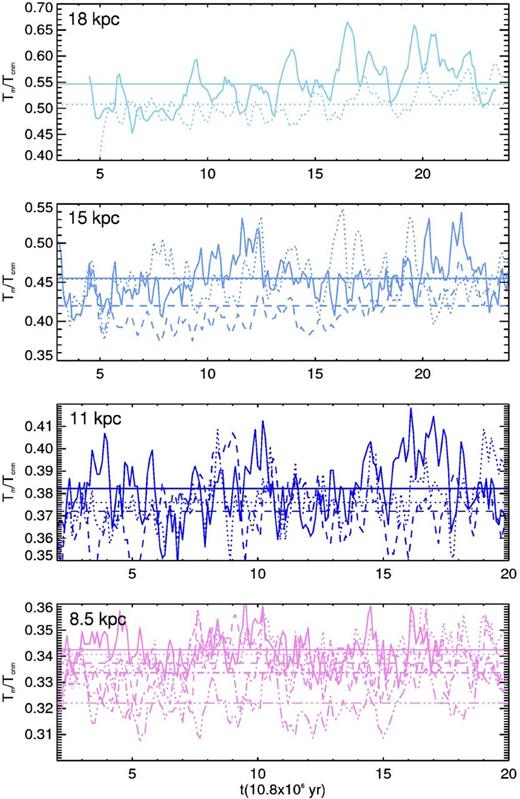
Evolution of the ratio Tm/Tcnm. The colour and line codes are the same as in Fig. 6.
As expected from the large difference between the ‘imposed’ value of the mean temperature and its real values (see Table 3), the resulting values of fm for all radii (Fig. 15), are smaller than fc. This reduction on the cold mass fraction is more dramatic for 8.5 and 11 kpc, indicating that there is a considerable mass contribution of the cold gas with T > 100 K, and that the contribution of this gas increases as Rg decreases.
Evolution of the cold gas mass fraction computed with the mean temperature criterion fm. The colour and line codes are the same as in Fig. 6.
4 DISCUSSION AND SUMMARY
The results presented in the previous section explore the cold mass fractions resulting when cooling functions and initial conditions adapted to describe the thermal conditions of the atomic gas in the Galactic mid-plane at Rg = 8.5, 11, 15 and 18 kpc are used. Other than cooling, our simulations only include forced turbulence at a scale of 50 pc. Varying the kinetic energy injection rate, we can control the rms velocity in our simulation box. This allows us to study the influence of vrms on the cold gas mass fraction at different Rg and to see to what extent this fraction can be controlled only by changing vrms within a range of values comparable with those observed in the H i gas. The main results that we obtain concern three main issues that we are going to discuss in the following three subsections.
4.1 The cold gas production at large Rg
For Rg = 15 and 18 kpc, there is a maximal velocity above which no CNM is formed. This is due to the augmentation of the cooling time which for the initial conditions increases by a factor of ∼13 and ∼23 when moving from 8.5 to 15 and 18 kpc, respectively. Because we are considering a relatively small perturbation scale, the maximal velocities for CNM formation could be larger in the real atomic ISM, depending on the energy injection scale, however larger perturbations have lower growth rates. The velocities required at large values of Rg to form CNM are subsonic, which brings the perturbations into a small-scale regime where thermally unstable density fluctuations can appear, giving rise to the development of a secondary instability. The growth rate of this instability is very low, but once it starts the mass of the cold phase increases considerably. Whether or not this phenomenon can play a role in the Galactic plane depends on the nature of the kinetic energy injection at large Galactocentric distances, in particular on the scale and on the frequency of this injection which are unknown. Concerning the scale, numerical simulations of a supernovae driven ISM with horizontal (vertical) scales of 1 kpc (2 kpc) at the solar radius find a correlation scale for the random flow of 100 pc for vertical distances up to 100 pc (Gent et al. 2013), but for the physical conditions at 15 and 18 kpc, due to the lower densities and SFRs, this scale could be different.
Taking into account that the cooling time increases very fast with Rg these behaviours could be also relevant in regions where turbulence is produced by mechanisms operating at larger scales. For three-dimensional isotropic turbulence, the maximal energy injection scale is of the order of the scale hight. This assumption is consistent with results by Kim, Kim & Ostriker (2006), who find that a stellar spiral potential perturbation induces gas motions on the scale of the vertical disc thickness. If we use the radial distribution of H estimated by Kalberla & Kerp (2009) for the H i, which implies that the scale hight increases by a factor of ∼1.94 and ∼2.64 when moving from the solar radius to 15 and 18 kpc, respectively, then, in order to maintain a constant ratio between the cooling time and the dynamical crossing time, the characteristic velocity of the perturbations should decrease by a factor of ∼7 and ∼9 for 15 and 18 kpc, respectively, at the temperatures that we use as initial conditions. For the velocity range that we considered for 8.5 kpc, this implies that for velocities between ∼0.3 and ∼2.5 km s−1 the instability regime at large Rg is similar to the one that we observe at 8.5 kpc. Note however that these velocities are smaller than velocity dispersions observed in the outer discs of nearby galaxies. In fact, Tamburro et al. (2009) found that in nearby spirals the random component of the vertical H i velocity dispersion σH declines exponentially with radius from ∼20 km s−1 to ∼5 km s−1, with a characteristic value at the optical radius (r25) ∼10 km s−1. Similar results concerning the radial decline of σH have been recently obtained by Ianjamasimanana et al. (2015) for a different sample. Then, even for larger perturbations it is possible that TI development at large Rg occurs at a similar regime to the one observed in our simulations.
4.2 The variation of the cold gas mass fraction with Rg
Our results show that simulations at 8.5 kpc with vrms = 7.84–17.43 km s−1 have an average one dimensional cold gas mass fractions, fx, close to the observed values for the solar neighbourhood. The volumetric cold gas fraction fc for the same radius is ∼0.60. For larger Rg, fx have also values close to the ones observed in the Galactic plane in two velocity regimes depending on Rg. For 11 kpc, supersonic perturbations with respect to the initial conditions are required, while at larger distances simulations with subsonic vrms have realistic values of fx. In these regimes fx is approximately constant with Rg as reported in observations. Although the trends of fc and fx with vrms are similar, we do not find any velocity combination giving a constant fc for Rg > 8.5 kpc. In contrast, the same two velocity regimes that give a constant fx, lead to a constant fx0, which is the average one-dimensional cold gas mass fractions considering only directions containing cold gas.
The presence of the two velocity regimes can be understood in terms of the temperature at which the cooling time equals the sound crossing time at the scale of the perturbations T50. At 11 kpc large pressure gradients are needed to have fx ∼ 0.1–0.2 because T50 is well above p0 at n0 (see Fig. 1) and the gas with T > T50 becomes stable. If the pressure gradient is not large enough then, the cold gas mass fraction becomes larger. In contrast, for 15 and 18 kpc T50 is close to the initial conditions and the pressure gradient caused by supersonic perturbations produces large amounts of gas with temperatures above T50 and small fractions of cold gas, while subsonic perturbations can approach an isobaric evolution leading to a larger fraction of cold gas. In these cases the development of the secondary instability further contributes to the cold gas mass fraction. Note that our cooling functions imply that for Rg = 15 and 18 kpc, the temperature at which τcool = τs is in the thermally unstable range for scales up to ∼180 and 500 pc, respectively.
4.3 The effects of different criteria for the CNM selection
We tested the effects of using different criteria to select the cold gas on the cold gas mass fraction. Interestingly, when we use a criterion that assumes pressure and thermal equilibrium (Section 3.3.1), the resulting volumetric cold mass fraction fp behaves in a similar way as does the averaged one dimensional mass fraction fx: It has values which are similar to those reported by observations and can have small variations with distances for Rg ≥ 11 kpc in the same velocity regimes as fx. This criterion leads to threshold temperatures for the cold gas between ∼100–170 K.
If a fixed temperature TT = 180 K is used to select the cold gas for the four values of Rg, the resulting cold gas mass fraction fT is lower than fc for Rg ≤ 15 kpc but follows the same radial trend, i.e. there is no a velocity regime where fT can have small radial variations with Rg. See Section 3.3.2.
Finally, for a criterion based on a fixed mean temperature (Section 3.3.3) leading to threshold temperatures ∼100 K, the resulting cold gas mass fraction fm becomes completely independent of Rg with values between 0.1 and 0.2. This means that the mass contribution of gas with T ≤ 100 K is independent of the cooling function and on the initial conditions as long as TI can develop. Of course this fact may change in the presence of self-gravity. The behaviour of fm does also indicate that when TI develops in a regime similar to the regime present at the solar radius, where the cooling time is considerably smaller than the dynamical time at unstable temperatures in thermal equilibrium, then the mass contribution of high temperature cold gas (T > 100 K) is very important.
5 CONCLUSIONS
Our results show that values of the average one-dimensional cold gas mass fraction fx are consistent with values reported by observations when velocity decreases with Rg. In particular, our simulations are able to reproduce an approximately constant cold mass fraction ∼0.1–0.2 for Galactocentric distances Rg going from 11 to 18 kpc when vrms becomes subsonic at large Rg. For 11 kpc, however, no velocity reduction, with respect to the value required to obtain a realistic mass fraction at 8.5 kpc, is needed to reproduce the observed values. This is partially consistent with the observed radial exponential decrease of the H i velocity dispersion in nearby galaxies because this kind of decline is not required, however it is compatible with the trend that is needed to reproduce the behaviour of fx. This implies that variations in the turbulent velocity could be at the origin of the observed radial behaviour of the one-dimensional cold gas mass fraction.
The comparison between fx and the volumetric mass fraction fc shows that the latter does not follow the same trend. At least for 50 pc perturbations we do not obtain any velocity regime for which fc is approximately constant for large Rg.
On the other hand, if the cold gas is selected by using a threshold temperature obtained by requiring the equality between the mean temperature of this gas and the equilibrium temperature at its mean pressure, the resulting volumetric cold gas mass fraction fp has values which are similar to those reported by observations and that follows the same trend with the Galactocentric radius if vrms decrease with Rg. However, the relationship between the observed cold gas mass fraction and fp remains unclear.
Finally we argue that the regime that we observe for the development of TI in our simulations at large Rg with small-scale 50 pc perturbations, which include the development of a secondary instability, can possibly be present in the outer parts of the Galactic Plane.
This work has been partially supported by UNAM-DGAPA grant IN110214. This work has made extensive use of the NASA's Astrophysics Data System Abstract Service.
REFERENCES
