


Abstract
The distribution of the orbital elements of the known extreme trans-Neptunian objects or ETNOs has been found to be statistically incompatible with that of an unperturbed asteroid population following heliocentric or, better, barycentric orbits. Such trends, if confirmed by future discoveries of ETNOs, strongly suggest that one or more massive perturbers could be located well beyond Pluto. Within the trans-Plutonian planets paradigm, the Planet Nine hypothesis has received much attention as a robust scenario to explain the observed clustering in physical space of the perihelia of seven ETNOs which also exhibit clustering in orbital pole position. Here, we revisit the subject of clustering in perihelia and poles of the known ETNOs using barycentric orbits, and study the visibility of the latest incarnation of the orbit of Planet Nine applying Monte Carlo techniques and focusing on the effects of the apsidal anti-alignment constraint. We provide visibility maps indicating the most likely location of this putative planet if it is near aphelion. We also show that the available data suggest that at least two massive perturbers are present beyond Pluto.
1 INTRODUCTION
The distribution of the orbital parameters of the known extreme trans-Neptunian objects or ETNOs is statistically incompatible with that of an unperturbed asteroid population following Keplerian orbits (de la Fuente Marcos & de la Fuente Marcos 2014, 2016b; Trujillo & Sheppard 2014; de la Fuente Marcos, de la Fuente Marcos & Aarseth 2015, 2016; Gomes, Soares & Brasser 2015; Batygin & Brown 2016; Brown & Batygin 2016; Malhotra, Volk & Wang 2016). A number of plausible explanations have been suggested. These include the possible existence of one (Trujillo & Sheppard 2014; Gomes et al. 2015; Batygin & Brown 2016; Brown & Batygin 2016; Malhotra et al. 2016) or more (de la Fuente Marcos & de la Fuente Marcos 2014, 2016b; de la Fuente Marcos et al. 2015, 2016) trans-Plutonian planets, capture of ETNOs within the Sun's natal open cluster (Jílková et al. 2015), stellar encounters (Brasser & Schwamb 2015; Feng & Bailer-Jones 2015), being a by-product of Neptune's migration (Brown & Firth 2016) or the result of the inclination instability (Madigan & McCourt 2016), and having been induced by Milgromian dynamics (Paučo & Klačka 2016).
At present, most if not all of the unexpected orbital patterns found for the known ETNOs seem to be compatible with the trans-Plutonian planets paradigm that predicts the presence of one or more planetary bodies well beyond Pluto. Within this paradigm, the best studied theoretical framework is that of the so-called Planet Nine hypothesis, originally suggested by Batygin & Brown (2016) and further developed in Brown & Batygin (2016). The goal of this analytically and numerically supported conjecture is not only to explain the observed clustering in physical space of the perihelia and the positions of the orbital poles of seven ETNOs (see Appendix A for further discussion), but also to account for other, previously puzzling, pieces of observational evidence like the existence of low perihelion objects moving in nearly perpendicular orbits. The Planet Nine hypothesis is compatible with existing data (Cowan, Holder & Kaib 2016; Fienga et al. 2016; Fortney et al. 2016; Ginzburg, Sari & Loeb 2016; Linder & Mordasini 2016) but, if Planet Nine exists, it cannot be too massive or bright to have escaped detection during the last two decades of surveys and astrometric studies (Luhman 2014; Cowan et al. 2016; Fienga et al. 2016; Fortney et al. 2016; Ginzburg et al. 2016; Linder & Mordasini 2016). A super-Earth in the sub-Neptunian mass range is most likely and such planet may have been scattered out of the region of the Jovian planets early in the history of the Solar system (Bromley & Kenyon 2016) or even captured from another planetary system (Li & Adams 2016; Mustill, Raymond & Davies 2016); super-Earths may also form at 125–750 au from the Sun (Kenyon & Bromley 2015, 2016).
The analysis of the visibility of Planet Nine presented in de la Fuente Marcos & de la Fuente Marcos (2016a) revealed probable locations of this putative planet based on data provided in Batygin & Brown (2016) and Fienga et al. (2016); the original data have been significantly updated in Brown & Batygin (2016). In addition, independent calculations (de la Fuente Marcos et al. 2016) show that the apsidal anti-alignment constraint originally discussed in Batygin & Brown (2016) plays a fundamental role on the dynamical impact of a putative Planet Nine on the orbital evolution of the known ETNOs. Here, we improve the results presented in de la Fuente Marcos & de la Fuente Marcos (2016a) focusing on the effects of the apsidal anti-alignment constraint. This paper is organized as follows. Section 2 presents an analysis of clustering in barycentric elements, pericentre and orbital pole positions, which is subsequently discussed. An updated evaluation of the visibility of Planet Nine virtual orbits at aphelion is given in Section 3. Conclusions are summarized in Section 4.
2 CLUSTERING IN BARYCENTRIC PARAMETERS
The six (Batygin & Brown 2016) or seven (Brown & Batygin 2016) ETNOs singled out within the Planet Nine hypothesis (see Appendix A for details) have a > 226 au (heliocentric) and they exhibit clustering in perihelion location in absolute terms and also in orbital pole position. In order to better understand the context of these clusterings we study the line of apsides of the known ETNOs (see Table 1 and Fig. 1) and the projection of their orbital poles on to the plane of the sky (see Table 1 and Fig. 2). Here, we consider barycentric orbits as it can be argued (see the discussion in Malhotra et al. 2016) that the use of barycentric orbital elements instead of the usual heliocentric ones is more correct in this case.

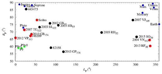
Poles of the objects in Table 1. Those singled out in Brown & Batygin (2016) are plotted in red, the known planets in blue, and various Planet Nine incarnations in green – P9v0 is the nominal solution in Batygin & Brown (2016), P9v1 is the one from Brown & Batygin (2016), and P9 is the previous one but enforcing apsidal anti-alignment.
In Trujillo & Sheppard (2014), the ETNOs are defined as asteroids with heliocentric semimajor axis greater than 150 au and perihelion greater than 30 au; at present, there are 16 known ETNOs. Because of the nature of their orbits, the ETNOs cannot experience a close approach to the known planets, including Neptune. Nevertheless, the orbits of the ETNOs are affected by indirect perturbations that induce variations in perihelion location. The perihelion distance of an ETNO depends on the value of its semimajor axis and eccentricity, e, as it is given by q = a(1 − e). However, its absolute position on the sky is only function of the inclination, i, the longitude of the ascending node, Ω, and the argument of perihelion, ω. In heliocentric ecliptic coordinates, the longitude and latitude of an object at perihelion, (lq, bq), are given by the expressions: tan (lq − Ω) = tan ω cos i and sin bq = sin ω sin i (see e.g. Murray & Dermott 1999). For an orbit with zero inclination, lq = Ω + ω and |$b_q=0^\circ$|; therefore, if |$i=0^\circ$|, the value of lq coincides with that of the longitude of perihelion parameter, ϖ = Ω + ω. In Brown & Batygin (2016), lq is called ‘perihelion longitude’ and bq is the ‘perihelion latitude’. Considering barycentric orbits, we denote the barycentric ecliptic coordinates of an ETNO at pericentre as (Lq, Bq). In Table 1 we show the values of q, Lq and Bq computed using the barycentric data in Table 2. The input values are from Jet Propulsion Laboratory's Small-Body Database1 (SBDB) and Horizons On-Line Ephemeris System (Giorgini et al. 1996).
Pericentre distances, q, ecliptic coordinates at pericentre, (Lq, Bq), and projected pole positions, (Lp, Bp), of the 16 objects discussed in this paper computed using barycentric orbits, see also Figs 1 and 2. (Epoch: 2457600.5, 2016 July 31.0 00:00:00.0 TDB. J2000.0 ecliptic and equinox. Input data from the SBDB; data as of 2016 July 13.)
| Object | q (au) | Lq (|$^\circ$|) | Bq (|$^\circ$|) | Lp (|$^\circ$|) | Bp (|$^\circ$|) |
|---|---|---|---|---|---|
| (82158) 2001 FP185 | 34.25 | 185.28 | 3.52 | 89.36 | 59.20 |
| (90377) Sedna | 76.19 | 96.31 | − 8.94 | 54.40 | 78.07 |
| (148209) 2000 CR105 | 44.12 | 87.28 | − 15.39 | 38.29 | 67.24 |
| (445473) 2010 VZ98 | 34.35 | 71.21 | − 3.26 | 27.40 | 85.49 |
| 2002 GB32 | 35.34 | 213.24 | 8.49 | 87.04 | 75.81 |
| 2003 HB57 | 38.10 | 208.32 | 2.88 | 107.87 | 74.50 |
| 2003 SS422 | 39.42 | 359.91 | − 8.28 | 61.05 | 73.21 |
| 2004 VN112 | 47.32 | 35.65 | − 13.59 | 336.02 | 64.45 |
| 2005 RH52 | 39.00 | 336.98 | 10.83 | 216.11 | 69.55 |
| 2007 TG422 | 35.56 | 39.41 | − 17.88 | 22.91 | 71.40 |
| 2007 VJ305 | 35.18 | 3.15 | − 4.40 | 294.38 | 78.02 |
| 2010 GB174 | 48.56 | 118.83 | − 4.65 | 40.71 | 68.44 |
| 2012 VP113 | 80.44 | 26.32 | − 21.94 | 0.80 | 65.95 |
| 2013 GP136 | 41.06 | 248.08 | 21.91 | 120.73 | 56.46 |
| 2013 RF98 | 36.28 | 27.88 | − 19.93 | 337.53 | 60.40 |
| 2015 SO20 | 33.17 | 28.89 | − 2.05 | 303.63 | 66.59 |
Barycentric orbital elements and parameters – q = a(1 − e), Q = a(1 + e) is the aphelion distance, ϖ = Ω + ω, P is the orbital period, Ω* and ω* are Ω and ω in the interval (−π, π) instead of the regular (0, 2π) – of the known ETNOs. The statistical parameters are Q1, first quartile, Q3, third quartile, IQR, interquartile range, OL, lower outlier limit (Q1 − 1.5IQR), and OU, upper outlier limit (Q3 + 1.5IQR). Input data as in Table 1.
| Object | a (au) | e | i (|$^\circ$|) | Ω (|$^\circ$|) | ω (|$^\circ$|) | ϖ (|$^\circ$|) | q (au) | Q (au) | P (yr) | Ω* (|$^\circ$|) | ω* (|$^\circ$|) |
|---|---|---|---|---|---|---|---|---|---|---|---|
| 82158 | 215.979 15 | 0.841 41 | 30.801 34 | 179.358 92 | 6.884 51 | 186.243 43 | 34.252 44 | 397.705 86 | 3172.011 64 | 179.358 92 | 6.884 51 |
| Sedna | 506.088 46 | 0.849 45 | 11.928 56 | 144.402 51 | 311.285 69 | 95.688 20 | 76.190 98 | 935.985 94 | 11 377.757 35 | 144.402 51 | − 48.714 31 |
| 148209 | 221.971 88 | 0.801 22 | 22.755 98 | 128.285 90 | 316.689 22 | 84.975 12 | 44.122 67 | 399.821 08 | 3304.942 85 | 128.285 90 | − 43.310 78 |
| 445473 | 153.361 00 | 0.776 02 | 4.510 50 | 117.398 58 | 313.725 57 | 71.124 15 | 34.350 48 | 272.371 52 | 1897.970 30 | 117.398 58 | − 46.274 43 |
| 2002 GB32 | 206.509 31 | 0.828 87 | 14.192 46 | 177.043 95 | 37.047 20 | 214.091 15 | 35.339 79 | 377.678 83 | 2965.694 98 | 177.043 95 | 37.047 20 |
| 2003 HB57 | 159.665 57 | 0.761 38 | 15.500 28 | 197.871 07 | 10.829 77 | 208.700 84 | 38.098 95 | 281.232 18 | 2016.201 47 | − 162.128 93 | 10.829 77 |
| 2003 SS422 | 197.895 67 | 0.800 78 | 16.785 97 | 151.046 90 | 209.928 64 | 0.975 54 | 39.424 55 | 356.366 79 | 2782.091 80 | 151.046 90 | − 150.071 36 |
| 2004 VN112 | 327.435 21 | 0.855 48 | 25.547 61 | 66.022 80 | 326.996 99 | 33.019 79 | 47.322 01 | 607.548 41 | 5921.136 75 | 66.022 80 | − 33.003 01 |
| 2005 RH52 | 153.677 48 | 0.746 24 | 20.445 77 | 306.110 67 | 32.538 53 | 338.649 20 | 38.997 10 | 268.357 86 | 1903.848 38 | − 53.889 33 | 32.538 53 |
| 2007 TG422 | 502.042 48 | 0.929 16 | 18.595 30 | 112.910 71 | 285.685 12 | 38.595 83 | 35.562 65 | 968.522 30 | 11 241.589 33 | 112.910 71 | − 74.314 88 |
| 2007 VJ305 | 192.099 34 | 0.816 84 | 11.983 76 | 24.382 39 | 338.334 91 | 2.717 30 | 35.184 70 | 349.013 98 | 2660.760 77 | 24.382 39 | − 21.665 09 |
| 2010 GB174 | 351.127 35 | 0.861 69 | 21.562 45 | 130.714 44 | 347.245 10 | 117.959 54 | 48.562 88 | 653.691 82 | 6575.276 41 | 130.714 44 | − 12.754 90 |
| 2012 VP113 | 263.165 64 | 0.694 36 | 24.051 55 | 90.803 92 | 293.549 65 | 24.353 57 | 80.435 15 | 445.896 13 | 4266.392 40 | 90.803 92 | − 66.450 35 |
| 2013 GP136 | 149.786 73 | 0.725 87 | 33.539 04 | 210.727 29 | 42.478 18 | 253.205 47 | 41.060 79 | 258.512 67 | 1832.006 56 | − 149.272 71 | 42.478 18 |
| 2013 RF98 | 317.065 25 | 0.885 57 | 29.600 66 | 67.533 81 | 316.375 28 | 23.909 09 | 36.282 42 | 597.848 08 | 5642.089 82 | 67.533 81 | − 43.624 72 |
| 2015 SO20 | 164.902 89 | 0.798 85 | 23.411 06 | 33.633 83 | 354.830 23 | 28.464 06 | 33.170 08 | 296.635 70 | 2116.213 17 | 33.633 83 | − 5.169 77 |
| Mean | 255.173 34 | 0.810 82 | 20.325 77 | 133.640 48 | 221.526 54 | 107.667 02 | 43.647 35 | 466.699 32 | 4354.749 00 | 66.140 48 | − 25.973 46 |
| Std. dev. | 116.486 33 | 0.061 05 | 7.724 95 | 71.950 62 | 140.157 70 | 102.408 43 | 14.310 74 | 226.780 10 | 3103.338 12 | 105.712 29 | 49.062 88 |
| Median | 211.244 23 | 0.809 03 | 21.004 11 | 129.500 17 | 302.417 67 | 78.049 63 | 38.548 02 | 387.692 35 | 3068.853 31 | 101.857 31 | − 27.334 05 |
| Q1 | 163.593 56 | 0.772 36 | 15.173 32 | 84.986 39 | 41.120 44 | 27.436 44 | 35.301 02 | 292.784 82 | 2091.210 24 | 31.320 97 | − 46.884 40 |
| Q3 | 319.657 74 | 0.850 96 | 24.425 56 | 177.622 69 | 319.266 16 | 191.857 78 | 44.922 51 | 600.273 17 | 5711.851 55 | 134.136 46 | 7.870 82 |
| IQR | 156.064 18 | 0.078 60 | 9.252 24 | 92.636 30 | 278.145 73 | 164.421 35 | 9.621 49 | 307.488 35 | 3620.641 31 | 102.815 49 | 54.755 23 |
| OL | − 70.502 72 | 0.654 46 | 1.294 96 | − 53.968 06 | − 376.098 15 | − 219.195 58 | 20.868 79 | − 168.447 70 | − 3339.751 72 | − 122.902 26 | − 129.017 24 |
| OU | 553.754 02 | 0.968 86 | 38.303 93 | 316.577 14 | 736.484 75 | 438.489 80 | 59.354 74 | 1061.505 68 | 11 142.813 51 | 288.359 69 | 90.003 66 |
| Statistics of Sedna, 148209, 2004VN112, 2007 TG422, 2010 GB174, 2012 VP113 and 2013 RF98 | |||||||||||
| Mean | 355.556 61 | 0.839 56 | 22.006 02 | 105.810 58 | 313.975 29 | 59.785 88 | 52.639 82 | 658.473 40 | 6904.169 27 | 105.810 58 | − 46.024 71 |
| Std. dev. | 110.144 55 | 0.074 77 | 5.602 87 | 31.460 21 | 20.470 89 | 38.763 57 | 18.275 09 | 220.425 83 | 3199.111 04 | 31.460 21 | 20.470 89 |
| Median | 327.435 21 | 0.855 48 | 22.755 98 | 112.910 71 | 316.375 28 | 38.595 83 | 47.322 01 | 607.548 41 | 5921.136 75 | 112.910 71 | − 43.624 72 |
| Q1 | 290.115 45 | 0.825 34 | 20.078 88 | 79.168 86 | 302.417 67 | 28.686 68 | 40.202 55 | 521.872 11 | 4954.241 11 | 79.168 86 | − 57.582 33 |
| Q3 | 426.584 91 | 0.873 63 | 24.799 58 | 129.500 17 | 321.843 10 | 90.331 66 | 62.376 93 | 794.838 88 | 8908.432 87 | 129.500 17 | − 38.156 90 |
| IQR | 136.469 47 | 0.048 29 | 4.720 70 | 50.331 31 | 19.425 43 | 61.644 98 | 22.174 38 | 272.966 77 | 3954.191 76 | 50.331 31 | 19.425 43 |
| OL | 85.411 24 | 0.752 90 | 12.997 82 | 3.671 90 | 273.279 52 | − 63.780 80 | 6.940 97 | 112.421 95 | − 977.046 53 | 3.671 90 | − 86.720 48 |
| OU | 631.289 12 | 0.946 07 | 31.880 63 | 204.997 13 | 350.981 25 | 182.799 14 | 95.638 51 | 1204.289 03 | 14 839.720 51 | 204.997 13 | − 9.018 75 |
Fig. 1 shows the position in the sky at pericentre as a function of the pericentre distance for the known ETNOs. The objects in Brown & Batygin (2016) are plotted in red; the average angular separation at pericentre for this group is 44|$^\circ$|±30|$^\circ$|, but the pair 2012 VP113–2013 RF98 has a separation of 2| $_{.}^{\circ}$|5, 2004 VN112–2007 TG422 has 5| $_{.}^{\circ}$|6, and 2004 VN112–2013 RF98 has 9| $_{.}^{\circ}$|8. In addition to this clustering, other obvious groupings are also visible. The dispersion of these additional groupings in ecliptic coordinates is similar to that of the set singled out by Brown & Batygin (2016), but their dispersion in q is considerably lower. ETNOs (82158) 2001 FP185, 2002 GB32 and 2003 HB57 have a nearly common line of apsides; the same can be said about (445473) 2010 VZ98, 2007 VJ305 and 2015 SO20. The case for the first grouping is particularly strong. Out of 16 known ETNOs, only five reach pericentre north from the ecliptic, i.e. |$B_q>0^\circ$|; these objects are 82158, 2002 GB32, 2003 HB57, 2005 RH52 and 2013 GP136. This represents a 2σ departure from an isotropic distribution in Bq, where |$\sigma =\sqrt{n}/2$| is the standard deviation for binomial statistics. This marginally significant result suggests that an unknown massive perturber has aligned the apsidal orientation of these objects, but the Planet Nine hypothesis cannot explain this pattern (Batygin & Brown 2016); another perturber is needed as the line of apsides is scarcely affected by indirect perturbations from the known planets. A nearly common line of apsides is also expected in a set of objects resulting from the break-up of a single object at pericentre. Such scenario might be linked to some of the groupings observed.
In Table 1 we show the current values of the position in the sky of the poles of the orbits of the known ETNOs computed using the data in Table 2; the ecliptic coordinates of the pole are |$(L_{\rm p}, B_{\rm p}) = (\Omega -90^\circ , 90^\circ -i)$|. Fig. 2 shows the poles of the known ETNOs and also those of the known planets of the Solar system and various nominal orbits of Planet Nine (epoch 2457600.5 JD). The objects singled out in Brown & Batygin (2016) and Planet Nine appear to exhibit a relative arrangement in terms of position of their orbital poles similar to the one existing between Neptune and Pluto. For this group, the average polar separation is 16|$^\circ$|±8|$^\circ$|, but the pair 148209–2010 GB174 has 1| $_{.}^{\circ}$|5, 2004 VN112–2013 RF98 has 4| $_{.}^{\circ}$|1, 148209–2007 TG422 has 6| $_{.}^{\circ}$|8, 2007 TG422–2010 GB174 has 6| $_{.}^{\circ}$|8, and 2007 TG422–2012 VP113 has 9| $_{.}^{\circ}$|6. On the other hand, the ETNOs 2002 GB32 and 2003 HB57 not only exhibit apsidal alignment but their orbital poles are also very close.
As for the overall clustering in orbital parameter space, it has been claimed that the ETNOs exhibit clustering in the values of their ω (Trujillo & Sheppard 2014), e and i (de la Fuente Marcos & de la Fuente Marcos 2014), and Ω (Brown & Firth 2016). Table 2 presents the descriptive statistics of the known ETNOs; in this table, unphysical values are shown for completeness. The bottom block of statistics in Table 2 (see also Appendix A) focuses on the seven ETNOs singled out in Brown & Batygin (2016). The overall statistics is only slightly different from that of the heliocentric orbital elements. The mean value of the barycentric e of the known ETNOs amounts to 0.81±0.06, the barycentric i is 20|$^\circ$|±8|$^\circ$|, the barycentric Ω is 134|$^\circ$|±72|$^\circ$|, and the barycentric ω is −26|$^\circ$|±49|$^\circ$|(see ω* in Table 2). Clustering in e may be due to selection effects, but the others cannot be explained as resulting from observational biases, they must have a dynamical origin (de la Fuente Marcos & de la Fuente Marcos 2014). For the ETNO sample in Brown & Batygin (2016), the average values of the barycentric orbital parameters are e = 0.84 ± 0.07, |$i=22^\circ \pm 6^\circ$|, |$\Omega =106^\circ \pm 31^\circ$| and |$\omega =314^\circ \pm 20^\circ$|.
Regarding the issue of statistical outliers and assuming that outliers are observations that fall below Q1 − 1.5 IQR or above Q3 + 1.5 IQR, where Q1 is the first quartile, Q3 is the third quartile, and IQR is the interquartile range, we observe a small but relevant number of outliers. For the entire sample, 2003 SS422 is an outlier in terms of ω* (see Table 2), Sedna and 2012 VP113 are outliers in terms of q, and Sedna and 2007 TG422 are outliers in terms of orbital period. In terms of size (not shown in the table), Sedna is a very significant outlier with H = 1.6 mag when the lower and upper limits for outliers are 4.7 mag and 8.7 mag, respectively. As for the sample of ETNOs in Brown & Batygin (2016), Sedna is an statistical outlier in terms of i.
3 VISIBILITY ANALYSIS
Here, we apply the Monte Carlo approach (Metropolis & Ulam 1949) described in de la Fuente Marcos & de la Fuente Marcos (2014) to construct visibility maps indicating the most probable location of this putative planet if it is near aphelion. Each Monte Carlo experiment consists of 107 test orbits uniformly distributed in parameter space. The analyses in e.g. Cowan et al. (2016), Fienga et al. (2016), Fortney et al. (2016), Ginzburg et al. (2016) and Linder & Mordasini (2016) strongly disfavour a present-day Planet Nine located at perihelion and they do not discard the aphelion which is also favoured in Brown & Batygin (2016).
3.1 Batygin & Brown (2016)
The resonant coupling mechanism described in Batygin & Brown (2016) emphasizes the existence of simultaneous apsidal anti-alignment and nodal alignment, i.e. Δϖ librates about 180|$^\circ$|and ΔΩ librates about 0|$^\circ$|. The relative values of ϖ and Ω of the ETNO with respect to those of the perturber must oscillate in order to maintain orbital confinement but see Beust (2016) for a detailed analysis. In Batygin & Brown (2016), the value of ω of the putative Planet Nine is 138|$^\circ$|±21|$^\circ$|. It is also indicated that the average value of Ω for their six ETNOs is 113|$^\circ$|±13|$^\circ$|and that of ω is 318|$^\circ$|±8|$^\circ$|. Applying the conditions for stability and using the other values discussed in their work, we generate a synthetic population of Planet Nines with a ∈ (400, 1500) au, e ∈ (0.5, 0.8), i ∈ (15, 45)|$^\circ$|, Ω ∈ (100, 126)|$^\circ$|and ω ∈ (117, 159)|$^\circ$|. Fig. 3, left-hand panels, shows the distribution in equatorial coordinates of the set of studied orbits. In this figure, the value of the parameter in the appropriate units is colour coded following the scale printed on the associated colour box. The location of the Galactic disc appears in panel D (inclination). The background stellar density is the highest towards this region. The distribution of Q, a and e is rather uniform as expected because the location in the sky of Planet Nine does not depend on these parameters (see above). The distribution in declination depends on i and ω; those orbits with higher values of i reach aphelion at lower declinations, the same behaviour is observed for the ones with lower values of ω. The location in right ascension mainly depends on the value of Ω, both increasing in direct proportion. Fig. 4, left-hand panels, shows that the frequency distribution in right ascension and declination is far from uniform; the probability of finding an orbit reaching aphelion is highest in the region limited by α ∈ (4.5, 5.5)h and |$\delta \in (6, 9)^\circ$|. However, the mean values of Ω and ω for the six ETNOs of interest differ from those in Table A1.
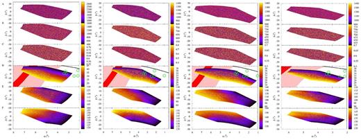
Distribution in equatorial coordinates of the aphelia of the studied orbits as a function of various orbital parameters: Q (panel A), a (panel B), e (panel C), i (panel D), Ω (panel E), and ω (panel F). The left-hand panels show results using the sets of orbits in Batygin & Brown (2016), those of orbits from Brown & Batygin (2016) are displayed in the second to left-hand panels; the second to right-hand panels and the right-hand panels focus on the set of orbits described in Section 3.3, imposing Δϖ ∼180|$^\circ$|and ΔΩ ∼0|$^\circ$| using the data in Tables 2 and A1, respectively. In panel D, the green circles give the location at discovery of known ETNOs (see table 2 in de la Fuente Marcos & de la Fuente Marcos 2016a), in red we have the Galactic disc that is arbitrarily defined as the region confined between galactic latitude −5|$^\circ$| and 5|$^\circ$|, in pink the region enclosed between galactic latitude −30|$^\circ$|and 30|$^\circ$|, and in black the ecliptic.
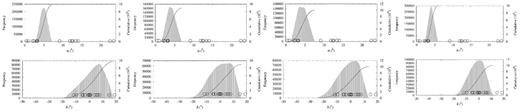
Frequency distribution in equatorial coordinates (right ascension, top panel, and declination, bottom panel) of the virtual orbits in Fig. 3. The number of bins is 2 n1/3, where n is the number of virtual orbits plotted, error bars are too small to be seen. The black circles correspond to data in table 2 of de la Fuente Marcos & de la Fuente Marcos (2016a).
| Parameter | a (au) | e | i (|$^\circ$|) | Ω (|$^\circ$|) | ω (|$^\circ$|) | ϖ (|$^\circ$|) | q (au) | Q (au) | P (yr) | Ω* (|$^\circ$|) | ω* (|$^\circ$|) |
|---|---|---|---|---|---|---|---|---|---|---|---|
| Mean | 377.820 73 | 0.845 95 | 21.881 02 | 102.064 70 | 313.522 97 | 55.587 67 | 54.059 35 | 701.582 11 | 7504.040 34 | 102.064 70 | − 46.477 03 |
| Std. dev. | 101.952 84 | 0.079 78 | 6.126 94 | 32.708 23 | 22.386 39 | 40.682 77 | 19.592 05 | 206.627 25 | 3042.773 93 | 32.708 23 | 22.386 39 |
| Median | 339.281 28 | 0.858 59 | 22.807 00 | 101.857 31 | 313.830 49 | 35.807 81 | 47.942 45 | 630.620 12 | 6248.206 58 | 101.857 31 | − 46.169 51 |
| Q1 | 319.657 74 | 0.850 96 | 19.337 09 | 73.351 33 | 297.983 66 | 26.520 12 | 39.042 32 | 600.273 17 | 5711.851 55 | 73.351 33 | − 62.016 34 |
| Q3 | 464.313 70 | 0.879 60 | 25.173 59 | 126.263 51 | 324.341 56 | 81.415 11 | 69.283 95 | 865.412 41 | 10 075.011 10 | 126.263 51 | − 35.658 44 |
| IQR | 144.655 95 | 0.028 64 | 5.836 50 | 52.912 17 | 26.357 90 | 54.894 98 | 30.241 63 | 265.139 24 | 4363.159 55 | 52.912 17 | 26.357 90 |
| OL | 102.673 81 | 0.807 99 | 10.582 33 | − 6.016 93 | 258.446 81 | − 55.822 35 | − 6.320 13 | 202.564 30 | − 832.887 77 | − 6.016 93 | − 101.553 19 |
| OU | 681.297 63 | 0.922 56 | 33.928 35 | 205.631 77 | 363.878 41 | 163.757 58 | 114.646 41 | 1263.121 27 | 16 619.750 42 | 205.631 77 | 3.878 41 |
3.2 Brown & Batygin (2016)
The Planet Nine hypothesis has been further developed in Brown & Batygin (2016). In this new work, the volume of orbital parameter space linked to the putative planet for an assumed mass of 10 M⊕ is enclosed by a ∈ (500, 800) au, e ∈ (0.32, 0.74), i ∈ (22, 40)|$^\circ$|, Ω ∈ (72.2, 121.2)|$^\circ$|and ω ∈ (120, 160)|$^\circ$|. Figs 3 and 4, second to left-hand panels, show similar trends to the previous ones but now the distribution in equatorial coordinates of the aphelia is wider. The probability is highest in the region limited by α ∈ (3, 5)h and |$\delta \in (-1, 10)^\circ$|. This enlarges the optimal search area significantly. However, they use a value of lq of 241|$^\circ$|±15|$^\circ$|that is based on a value of 61|$^\circ$| for the seven ETNOs so Δlq – not Δϖ – librates about 180|$^\circ$|; the average value of lq for these ETNOs from Table 1 is 62|$^\circ$|±38|$^\circ$|, the average value of ϖ is 60|$^\circ$|±39|$^\circ$|.
3.3 Enforcing apsidal anti-alignment
Here, we enforce apsidal anti-alignment and nodal alignment, using the data in Table 2, bottom section, and considering the Planet Nine orbital parameter domain defined by a ∈ (600, 800) au, e ∈ (0.5, 0.7), i ∈ (22, 40)|$^\circ$|, Ω ∈ (74.4, 137.3)|$^\circ$|and ω ∈ (113.5, 154.4)|$^\circ$|. Figs 3 and 4, second to right-hand panels, show that in this scenario, Planet Nine is most likely to be moving within α ∈ (3.0, 5.5)h and |$\delta \in (-1, 6)^\circ$|, if it is near aphelion. If the data in Table A1 are used instead, then Ω ∈ (87, 117)|$^\circ$|and ω ∈ (118.5, 148.8)|$^\circ$|and we obtain Figs 3 and 4, right-hand panels. In this case, the putative planet is most likely moving within α ∈ (3.5, 4.5)h and |$\delta \in (-1, 2)^\circ$|, i.e. projected towards the separation between the constellations of Taurus and Eridanus. In terms of probability, now the most likely location of Planet Nine is at α ∼ 4h and δ ∼ 0| $_{.}^{\circ}$|5, in Taurus. This area is compatible with Orbit A in de la Fuente Marcos et al. (2016).
4 CONCLUSIONS
In this paper, we have re-analysed the various clusterings in ETNO orbital parameter space claimed in the literature and explored the visibility of Planet Nine within the context of improved constraints. Our results confirm the findings in Batygin & Brown (2016) and Brown & Batygin (2016) regarding clustering but using barycentric orbits. However, the observed overall level of clustering may not be maintained by a putative Planet Nine alone, other perturbers should exist. Summarizing:
We confirm the existence of apsidal alignment and similar projected pole orientations among the currently known ETNOs. These patterns are consistent with the presence of perturbers beyond Pluto and/or, less likely, break-up of large asteroids at perihelion.
If Planet Nine is at aphelion, it is most likely moving within α ∈ (3.0, 5.5)h and |$\delta \in (-1, 6)^\circ$| if Δϖ ∼180|$^\circ$|and ΔΩ ∼0|$^\circ$|.
We thank two anonymous referees for their constructive reports, and S. J. Aarseth, D. P. Whitmire, G. Carraro, D. Fabrycky, A. V. Tutukov, S. Mashchenko, S. Deen and J. Higley for comments on ETNOs and trans-Plutonian planets. This work was partially supported by the Spanish ‘Comunidad de Madrid’ under grant CAM S2009/ESP-1496. In preparation of this paper, we made use of the NASA Astrophysics Data System, the ASTRO-PH e-print server and the MPC data server.
REFERENCES
APPENDIX A: Further details on the comparison with the results of Brown & Batygin (2016)
According to the heliocentric orbital solutions publicly available from the SBDB, the six (not seven) objects singled out in Batygin & Brown (2016) all have values of the heliocentric semimajor axis, a, larger than 257 au; Brown & Batygin (2016) indicate that their semimajor axes are larger than 227 au. The six original objects in Batygin & Brown (2016) – namely, (90377) Sedna (a = 499 au), 2004 VN112 (a = 318 au), 2007 TG422 (a = 483 au), 2010 GB174 (a = 370 au), 2012 VP113 (a = 258 au) and 2013 RF98 (a = 307 au) – do not have the largest values of the perihelion distance, only four of them – Sedna (q = 76 au), 2004 VN112 (q = 47 au), 2010 GB174 (q = 49 au) and 2012 VP113 (q = 80 au) – are in this situation. In Brown & Batygin (2016), it is said that the seven objects with a > 227 au are singled out. However, fig. 1(a) in Brown & Batygin (2016) highlights in red only six objects (those singled out in Batygin & Brown 2016), not seven; (148209) 2000 CR105 (a = 226 au, q = 44 au), which has the eighth largest value of the heliocentric semimajor axis and the fifth largest perihelion distance, appears in green in that figure. The ETNO with the seventh largest value of the heliocentric semimajor axis is (82158) 2001 FP185 (a = 227 au, q = 34 au), not 148209 as erroneously stated in Brown & Batygin (2016). Our analysis in Figs 1 and 2 shows that 82158 is unlikely to be dynamically connected with the original six ETNOs singled out in Batygin & Brown (2016), but 148209 very probably is. Therefore, the seven objects of interest within the context of the Planet Nine hypothesis are: Sedna, 148209, 2004VN112, 2007 TG422, 2010 GB174, 2012 VP113 and 2013 RF98.
In terms of barycentric (not heliocentric) orbits, see Table 2, 148209 has the seventh largest value of the semimajor axis and 82158 has the eighth largest.
Table A1 shows the statistics for the six original objects in Batygin & Brown (2016); the average values of the orbital parameters are e = 0.85 ± 0.08, |$i=22^\circ \pm 6^\circ$|, |$\Omega =102^\circ \pm 33^\circ$| and |$\omega =314^\circ \pm 22^\circ$| (these values have been used in the discussion in Section 3.1). The average angular separation at pericentre for this group is 45|$^\circ$|±34|$^\circ$|and the average polar separation is 16|$^\circ$|±8|$^\circ$|. For the sample of ETNOs in Batygin & Brown (2016), both 2007 TG422 and 2012 VP113 are statistical outliers in terms of e (see Tables 2 and A1).
The expression for the eccentricity of the putative Planet Nine in Brown & Batygin (2016) produces negative values for masses under ∼6.38 M⊕ and the lower limit of the value of the semimajor axis. Production of unphysical values is the main reason why it has not been applied to select the range in eccentricities used in Section 3.3.
