


Abstract
On 2015 June 15, the black hole X-ray binary V404 Cygni went into outburst, exhibiting extreme X-ray variability which culminated in a final flare on June 26. Over the following days, the Swift-X-ray Telescope detected a series of bright rings, comprising five main components that expanded and faded with time, caused by X-rays scattered from the otherwise unobservable dust layers in the interstellar medium in the direction of the source. Simple geometrical modelling of the rings’ angular evolution reveals that they have a common temporal origin, coincident with the final, brightest flare seen by INTEGRAL's JEM X-1, which reached a 3–10 keV flux of ∼25 Crab. The high quality of the data allows the dust properties and density distribution along the line of sight to the source to be estimated. Using the Rayleigh–Gans approximation for the dust scattering cross-section and a power-law distribution of grain sizes a, ∝ a−q, the average dust emission is well modelled by |$q = 3.90^{+0.09}_{-0.08}$| and maximum grain size of |$a_+ = 0.147^{+0.024}_{-0.004} {\rm \ \mu m}$|, though significant variations in q are seen between the rings. The recovered dust density distribution shows five peaks associated with the dense sheets responsible for the rings at distances ranging from 1.19 to 2.13 kpc, with thicknesses of ∼40–80 pc and a maximum density occurring at the location of the nearest sheet. We find a dust column density of Ndust ≈ (2.0–2.5) × 1011 cm−2, consistent with the optical extinction to the source. Comparison of the inner rings’ azimuthal X-ray evolution with archival Wide-field Infrared Survey Explorer mid-IR data suggests that the second most distant ring follows the general IR emission trend, which increases in brightness towards the Galactic north side of the source.
1 INTRODUCTION
Diffuse haloes can be seen around X-ray sources when the column density to the source is sufficiently high that dust in the interstellar medium (ISM) scatters photons, originally emitted at small angles to the line of sight, towards the observer. The existence of such X-ray haloes was first proposed by Overbeck (1965) and their theoretical underpinnings have since been well developed (e.g. Mauche & Gorenstein 1986; Mathis & Lee 1991; Smith & Dwek 1998; Draine 2003b).
For a constant source of X-rays, scattered photons produce an extended component which broadens the radial profile beyond that of a typical point source. Detailed modelling of the halo profiles allows important information about the dust grains to be inferred, such as their composition, size and spatial distribution. Surveys conducted by ROSAT (Predehl & Schmitt 1995) and, more recently, Chandra/XMM–Newton (Valencic & Smith 2015), revealed that many absorbed sources have detectable X-ray haloes.
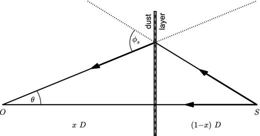
Assumed geometry for single scattering of X-rays from a thin layer of dust. The X-ray source, S, is at a distance D from the observer, O. The dust layer is at a fractional distance 1 − x from the source and scatters photons back towards the observer where they are seen at an angle θ to the original line of sight. The angle ϕs is the scattering angle.
This means that a bright, short duration flare, originating from the source at time t0, can produce a scattering ring whose radius increases with time, t, according to (t − t0)1/2. Such expanding rings have been seen around gamma-ray bursts (Vaughan et al. 2004, 2006; Tiengo & Mereghetti 2006), the magnetar 1E 1547−5408 (Tiengo et al. 2010) and the Galactic X-ray binary Cir X-1 (Heinz et al. 2015).
V404 Cyg is a black hole X-ray binary system (BHXB), last seen in outburst in 1989, when it was discovered to be a highly variable X-ray transient by the Ginga satellite (Tanaka 1989; Kitamoto 1990), flaring to an intensity of ∼20 Crab in the 1–37 keV energy range. Follow-up quiescent optical spectroscopy and infrared (IR) photometry allowed accurate binary parameters to be determined, revealing that the system contains a 12 ± 3 M⊙ black hole primary (Casares & Charles 1994; Shahbaz et al. 1994). Using radio VLBI observations, Miller-Jones et al. (2009) measured an accurate parallax for the source which gave a distance of 2.39 ± 0.14 kpc.
Situated at Galactic coordinates l, b = 73| $_{.}^{\circ}$|12, −2| $_{.}^{\circ}$|09, V404 Cyg lies near the Galactic plane. Hynes et al. (2009) modelled its quiescent multiwavelength spectral energy distribution (SED) and found a best-fitting optical reddening of AV = 4.0 (with a range 3.6–4.4). This implies a total (i.e. neutral plus molecular hydrogen) column density to the source of 8.1 × 1021 cm−2 (Kalberla et al. 2005; Willingale et al. 2013).
The Swift Burst Alert Telescope (BAT; Barthelmy et al. 2005) detected the first signs of renewed activity from V404 Cyg on 2015 June 15 at 18:31:38 ut (Barthelmy et al. 2015a).1 On this occasion, Swift slewed immediately to the source and the X-ray Telescope (XRT; Burrows et al. 2005) measured a 0.5–10 keV count rate of 1.0 count s−1, some ∼75 times brighter than the average quiescence rate seen in 2012 (e.g. Bernardini & Cackett 2014).
BAT triggered on the source a further five times during the course of the outburst (Barthelmy & Sbarufatti 2015; Barthelmy et al. 2015b,c; Cummings et al. 2015; Kennea et al. 2015), in which the flux increased significantly each time, as the BAT trigger criterion requires the count rate of a known source to be at least 2.5 times higher than the previous automatically updated trigger level.
With such a high column density along the line of sight, together with a highly variable X-ray source during outburst, the prospect of seeing the effects of dust scattering around V404 Cyg were good and this was, indeed, found to be the case when we reported the detection of multiple scattering rings around the source (Beardmore et al. 2015).
In this paper, we provide a detailed analysis of the Swift-XRT observations of the dust scattering rings around V404 Cyg. While our paper was being finalized we became aware of the work of Vasilopoulos & Petropoulou (2016, hereafter VP15), who also analysed the publicly available XRT data on the rings. Our modelling differs from theirs and employs a technique to recover the dust density distribution along the line of sight to the X-ray source. Further comparisons with the results of VP15 are made throughout the paper.
Section 2 describes the X-ray observations, as well as our data analysis methods and reports the results obtained from our radial/azimuthal profile and spectral analysis of the rings. Section 3 details our approach to the radial profile modelling, which provides an estimate of the dust density distribution to the source. Finally, Section 4 discusses the location of V404 Cyg in the context of the nearby Galactic environment and compares the X-ray observations with archival IR data.
2 OBSERVATIONS AND ANALYSIS
A series of Swift Target of Opportunity (ToO) observations were performed after the first BAT trigger, leading to the accumulation of 142 ks of XRT data over the next 43 d, with 86 ks collected in Photon Counting (PC) mode and the remaining 56 ks in Windowed Timing (WT) mode; the latter being used when the central source was bright. In the analysis that follows the XRT data were initially processed by the Swift software tools version 4.4 (from heasoft version 6.16), using the XRT gain calibration files released on 2015 July 21.
The 0.5–10.0 keV XRT light curve from the central source is shown in Fig. 2(a). The light curve was created from grade 0 events for WT mode, as this helps lessen the effects of pile-up for bright point sources (which becomes important above ∼100 count s−1 in this mode), and grade 0–12 events for PC mode. Appropriate corrections for (sometimes severe) pile-up were made to the data when necessary. We note the peak count rates in the XRT light curve published by VP15 are much lower than those presented here, indicating that pile-up was not correctly accounted for in their analysis. The PC data taken after day 14 were background subtracted using events extracted from an annular region located inside the innermost dust scattering ring. Also, given that the WT data from the central source could be affected by emission from the dust scattering halo (see for example, Fig. 3) – most notably when a strong X-ray flare was followed by a drop in the source count rate below ∼100 count s−1 – the halo contribution was subtracted using events extracted from a 30–60 pixel wide strip chosen to avoid the central point source, whenever possible. The y-axis of Fig. 2(a) is logarithmically scaled in order to show the highly variable nature of the soft X-ray flux from the central BHXB, which changed in brightness by five orders of magnitudes as it flared during this outburst. The highest count rate recorded by the XRT occurred between 10.754–10.771 d after the BAT trigger, in which the 0.5–10.0 keV flux peaked at an estimated ∼20 Crab. After day 11, the XRT light curve started a slow decline towards quiescent flux levels, which were reached approximately 50–65 d after the initial BAT trigger (Sivakoff et al. 2015).
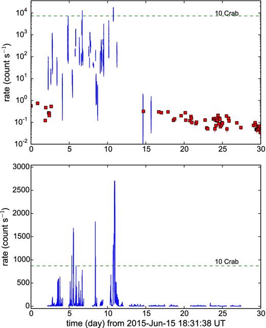
Upper panel (a): Swift-XRT 0.5–10.0 keV X-ray light curve from the central BHXB in V404 Cyg. PC mode data are plotted as squares to distinguish them from WT mode. Lower panel (b): INTEGRAL JEM X-1 3–10 keV light curve. The dashed horizontal lines mark the estimated ten Crab flux levels.
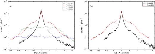
1D WT detector profiles from V404 Cyg calculated over the restricted energy band of 0.7–3.0 keV, chosen to emphasize the soft dust scattering emission over that of the harder central source. (a) The profile obtained on day 2.790 (solid line) is that expected for a typical point source. Following the final flare, the profiles from days 11.229 (dashed), 11.628 (dash–dotted), 13.226 (dotted) revealed extended emission from multiple rings associated with a dust scattering halo, which expand and fade with time. (b) Comparison of the halo profiles taken at a comparable time after the two brightest INTEGRAL detected flares, indicating the halo on day 11.229 (dashed) was four times brighter than the one on day 5.836 (solid), consistent with ratio of the fluences from the two flares (see Section 2.1).
ESA's INTEGRAL observatory (Winkler et al. 2003) began observing V404 Cyg through a number of ToO observations, starting two days after the BAT trigger. Fig. 2(b) shows the JEM X-1 (Lund et al. 2003) 3–10 keV light curve, made publicly available through the INTEGRAL Science Data Centre (ISDC; Kuulkers 2015a,b). The data were processed using version 10.2 of the ISDC Off-line Scientific Analysis (osa) software and calibration files. The temporal coverage of the INTEGRAL observations (total exposure 1276 ks) were higher than those of Swift, as the former has a longer orbital period and V404 Cyg was monitored with a greater cadence, and revealed a number of additional flaring episodes (e.g. Ferrigno et al. 2015a,b; Rodriguez et al. 2015a,b; Domingo et al. 2015). The most intense flare seen by JEM X-1 peaked at ∼25 Crab from day 10.882–10.987 and was the last bright flare of the outburst.
Similar large intensity variations and high flux levels ( ≳ 30 Crab) were seen by the higher energy Swift BAT and INTEGRAL IBIS (Ubertini et al. 2003) instruments (Rodriguez et al. 2015a; Segreto et al. 2015), though we note that, due to the strong energy dependence (∝ E−2) of the scattering cross-section (e.g. Draine 2003b), dust scattering preferentially responds to the soft X-ray flux which, at times, can be heavily absorbed.
As the X-ray light curve decayed after the final flaring activity from the central source, the XRT 1D WT detector profiles showed evidence for significantly extended wings, which increased in size and faded with time (see Fig. 3a), indicative of a dust scattering halo.
Once this became apparent, we requested that the XRT observations be switched to PC mode, whose 2D imaging capabilities confirmed the presence of multiple dust scattering rings (Beardmore et al. 2015). A series of 0.5–5.0 keV images from a subset of the PC mode observations are shown in Fig. 4, revealing the best example of expanding and fading dust scattering rings seen to date by any X-ray observatory.
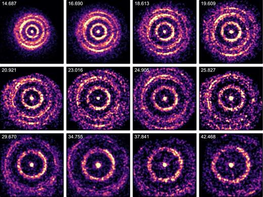
Representative Swift-XRT 0.5–5.0 keV exposure corrected images of the V404 Cyg field showing the expanding rings. Each image is 23.57 arcmin square (with north up and east to the left) and labelled with the mid-point time (days since the BAT trigger) in the upper left. The images have been smoothed by convolution with a Gaussian of σ = 4 pixels and are logarithmically scaled with a maximum value of 3.25 × 10⁻³ Δt−1.9 (count s−1 pixel−1), where Δt is the time in days since the ring-forming flare (see Section 2.1).
2.1 Radial profiles
As Swift is in a low Earth orbit and slews to multiple targets per orbit in order to optimize its observing schedule, observations of a particular source are broken up into one or more ‘snaphots’ of continuous exposure lasting up to ∼2 ks. At early times (day 14.6–20.5), images were created from single snapshots of XRT data, with typical exposure ranging from 0.8 to 1.7 ks. At later times, data from nearby snapshots were summed to increase the halo signal, leading to exposures up to 5.3 ks (day 29.7). The temporal spreading of the middle ring caused by the image creation was limited to 0.3 arcsec on day 14.7, 2.4 arcsec on day 23.0 and 9.1 arcsec on day 29.7. The outermost ring fell completely outside the XRT field of view after day 29.7, which provided a cut-off point for our analysis, though the inner rings were still visible after this time (see Fig. 4).
To analyse the rings in more detail, images were extracted over the energy range 1.0–4.0 keV. This restricted band was chosen to maximize the signal around the peak of the dust scattered spectrum while ensuring the majority of the halo photons arise from single scatterings, as multiple scatterings, which for a column density of 8 × 21 cm−2 become important below ∼ 1 keV (e.g. Mathis & Lee 1991; Smith et al. 2006), could broaden the halo. Furthermore, the analytical Rayleigh–Gans (RG) approximation for the dust scattering cross-section, used later when modelling the rings (Section 3), is applicable above ≳ 1 keV (e.g. Smith & Dwek 1998).
Radial profiles were then created about the central source position, the centroid of which had been determined by fitting the exposure corrected XRT point spread function (PSF) to each image. The exposures in each of the annular regions of the profiles were estimated using exposure maps which took into account the CCD bad-columns and removed hot-pixels, as well as the telescope vignetting function (calculated at 1.5 keV). Example radial profiles are shown in Fig. 5 and reveal considerable structure, with five resolvable large peaks associated with the rings, as well as other lower intensity emission, which are seen to expand with time.
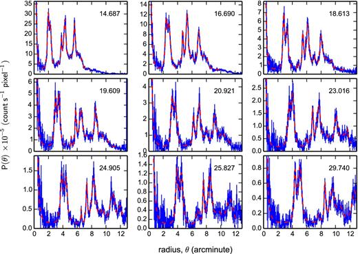
Example radial profiles created from 1.0–4.0 keV images. θ is the angular radius (arcmin) and P(θ) the measured surface brightness (count s−1 pixel−1) in the annulus at θ. Each panel is labelled with the image mid-point time (days since the BAT trigger, 2015 June 15 18:31:38 ut) in the upper-right corner. The dashed curve shows the best-fitting model, described in the text, which was used to measure the position of the five main rings.
The angular evolution of the rings recovered from the radial profile fitting is shown in Fig. 6. The figure also includes points estimated from the WT 1D profiles taken after the flare responsible for the rings, for comparison. These were calculated by creating a 2D model consisting of two uniform emission annular regions (representing rings 1 + 2 and 3 + 4 + 5, as the WT profiles cannot resolve the individual rings) plus a central source, which was then convolved with the XRT PSF and collapsed in 1D to mimic the WT readout, then fit to the 1D profiles to recover the centre of each annulus. The WT derived average ring locations are in good agreement with the PC data around day 14.687 and confirm the rings angular radius evolution immediately after the flare.

Angular radius evolution of the five main rings. The rings, R1, …, R5, are plotted from bottom to top, with symbols identified in the legend. Error bars are included but are typically smaller than the size of the symbol. The dashed lines show the best-fitting models, described in the text, whose parameters are marked in the legend. The diamonds show ring positions estimated from the WT data, for comparison, which were not used in the fitting.
Best-fitting flare time, t0 (days since BAT trigger), dust scattering slab fractional distance, x, and absolute distance, xD (pc). The t0 and x uncertainties are calculated at the 90 per cent confidence level, while those on xD are dominated by the uncertainty in the distance to the source. The first five rows show the fit results obtained when t0 was tied between the rings (χ2/ν = 108.5/104) and the last five when t0 was allowed to vary (χ2/ν = 100.8/100).
| Ring | t0 | x | xD |
|---|---|---|---|
| 1 | 10.932 ± 0.027 | 0.8899 ± 0.0008 | 2127 ± 125 |
| 2 | 0.8577 ± 0.0008 | 2050 ± 120 | |
| 3 | 0.6821 ± 0.0004 | 1630 ± 95 | |
| 4 | 0.6296 ± 0.0012 | 1505 ± 88 | |
| 5 | 0.4966 ± 0.0012 | 1187 ± 70 | |
| 1 | 11.052 ± 0.110 | 0.8885 ± 0.0008 | 2124 ± 124 |
| 2 | 11.024 ± 0.110 | 0.8565 ± 0.0023 | 2047 ± 120 |
| 3 | 10.919 ± 0.041 | 0.6824 ± 0.0012 | 1631 ± 96 |
| 4 | 10.893 ± 0.041 | 0.6306 ± 0.0012 | 1507 ± 88 |
| 5 | 10.946 ± 0.041 | 0.4962 ± 0.0012 | 1186 ± 70 |
The absolute distances of the ring forming slabs are also included in Table 1, with uncertainties dominated by the error on the distance to V404 Cyg. The dust sheets responsible for the rings occur at distances ranging from 1.19 to 2.13 kpc from Earth.
The mean t0 from Table 1 of VP15 occurs just 0.036 d before ours, with an rms of 0.054 d, so is completely consistent with our estimate, though they then assumed a flare time which was 0.085 d later when estimating the ring distances.
The predicted flare time of t0 = 10.932 d post BAT trigger, corresponding to 2015 Jun 26 16:54 ut, occurred during a gap in the XRT coverage. However, the INTEGRAL observatory was monitoring the source at this time. Fig. 7 shows an expanded view of the JEM X-1 3–10 keV light curve and reveals the measured t0 is at the centre of the brightest flare from the entire outburst. The flare has a 3–10 keV flux of ∼25 Crab and lasts for a duration (from fast rise to fast fall) of 0.106 d (9160 s), consistent with the estimate derived from the angular width of ring 3, and is undoubtedly responsible for the expanding dust scattering halo rings subsequently observed.
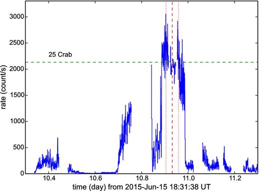
INTEGRAL JEM X-1 3–10 keV light curve showing the large flare coincident with the best-fitting t0 (dashed vertical line) and its associated uncertainty (dotted vertical lines). The horizontal dashed line marks the 25 Crab flux level. The gap from day 10.756 to 10.841 was caused by a high voltage shut down on the detector (see text).
We note that the gap in the JEM X-1 coverage from day 10.756–10.841 was caused by a high voltage power shutdown on the detector. This gap might be hiding additional fluence from the flare, as indicated by INTEGRAL's higher energy IBIS detector, which would increase the duration estimate closer to 0.2 d; though examination of the hardness ratio suggests the spectrum was harder at this time.
The higher cadence of data taken by INTEGRAL shows that V404 Cyg experienced a number of flaring episodes (Rodriguez et al. 2015a), each capable of forming dust scattering rings with an intensity proportional to the soft X-ray flare fluence. The next highest fluence flare seen by JEM X-1 occurred on day 5.547, lasted for a duration of approximately 0.059 d and reached a mean peak flux of 13 Crab. Assuming the flares are spectrally similar, the fluence in this flare was a factor of 3.5 times smaller than the final ring forming flare. VP15 performed a similar analysis but used the hard band (20–60 keV) INTEGRAL ISGRI data, which is not necessarily representative of the soft band flux given the spectral complexity of the flaring source, and estimated a factor of 3 reduction in flare fluence.
While XRT was not observing V404 Cyg at the time of the earlier flare, it did take a snapshot of data 0.289 d later on day 5.836. Fig. 3(b) compares the WT 1D profile at this time with one taken at approximately the same time after the bright flare (day 11.229). The wings of the profiles at 1 arcmin from the source reveal the halo flux from the earlier flare is a factor of ∼4.25 times fainter; that is, 40 per cent lower than the hard band derived fluence estimates.
Inspection of other snapshots of WT data revealed that many showed the effects of dust scattering haloes in their 1D profiles, especially after a flaring episode when the central source flux had dropped. Thus, we warn others interested in these data that care needs to be exercised when dealing with WT spectra from the central source to ensure the contribution from the halo is accounted for.
The halo emission from earlier flares contributes to the overall background level of the radial profiles following the final flare. However, the effect is relatively minor – for example, we estimate that the INTEGRAL flare seen on day 5.547 will contribute a maximum of 8 × 10⁻⁶ count s−1 pixel−1 at a radius of 3.5 arcmin (i.e. 15 per cent of the locally observed emission level of 5 × 10⁻⁵ count s−1 pixel−1) on day 14.687 (i.e. corresponding to the first profile in Fig. 5). The soft X-ray fluences from the other flares are lower and they contribute even less by the time of the PC mode observations of the rings.
2.2 Azimuthal profiles
The images in Fig. 4 show evidence for brightness variations around the rings. In order to characterize this behaviour, average azimuthal profiles for the five rings were created from the images over different times. The profiles were calculated using annuli of fixed width 16.5 arcsec (i.e. twice the XRT PSF FWHM; Moretti et al. 2005), centred on the rings as they evolved, and chosen to be small enough to avoid significant contamination from nearby rings. Also, while the profiles were exposure corrected using the vignetting corrected exposure maps, relatively large angular bins of size 20° were used to ensure any individual bins were not completely dominated by the detector bad columns.
The normalized azimuthal profiles, shown in Fig. 8, reveal greater than 50 per cent variations in the intensities of the rings as a function of azimuthal angle, ϕ (measured anticlockwise from equatorial west), with minima occurring between angles of ϕ ∼ 170° and 200°. The maximum azimuthal intensity for inner rings 1 and 2 are well separated (∼90°) even though they are radially close together, which suggests that they are formed in distinct dust scattering slabs. The outer ring, R5, has a double peaked azimuthal profile, with maxima at angles of 80° and 270° and shows a factor of 4 change in brightness around the ring.
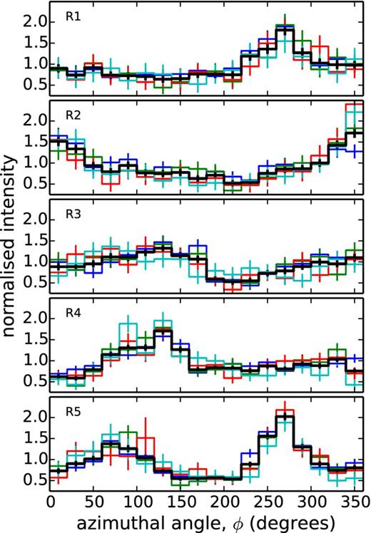
Averaged normalized azimuthal profiles for the five rings (R1, …, R5). The azimuthal angle (ϕ) is measured anticlockwise from the equatorial west direction. The colours refer to time intervals from day 14.69 to 17.03 (blue), 17.89 to 19.61 (green), 20.15 to 21.61 (red) and 22.74 to 25.83 (cyan). The thicker (black) lines show the overall average profiles from day 14.69 to 25.83.
Changes in the mean azimuthal profiles with time are evident from Fig. 8. This was most noticeable for ring 2, which revealed a clear variation in its peak azimuthal profile intensity that increased by ≳ 40 per cent once it had expanded beyond a radius of 3 arcmin.
The Galactic north/south line runs through azimuthal angles 35°/215°. Of the profiles in Fig. 8, the maximum from ring 2 appears to align the closest with the Galactic north direction, as might be expected if the column density were increasing towards the Galactic plane. Further discussion is deferred to Section 4.1.
VP15 also noted the presence of azimuthal structure in the XRT halo data; however, they did not separate out the behaviour of rings 1 + 2 or 3 + 4, or proceed to discuss the findings in any depth.
2.3 Halo spectral analysis
Spectra from the rings were extracted from the longest PC mode snapshots, or adjacent snapshots, using annular extraction regions tuned specifically for each case. Given their relative separations, spectra from rings 1 and 2 were extracted as one, which increased the statistical quality of the data. The same was done for rings 3 and 4. PC event grades 0–12 were selected for the spectra.
As the rings dominate the field of view and leave limited space on the detector from which to extract a good quality background spectrum, the PC mode observations from 2012 (total exposure 132 ks) were used to obtain an accurate non-halo background spectrum, which was extracted using an annulus of size 2.95–7.66 arcmin centred on the source, after five faint background point sources were removed. (Note, the background sources were too faint to have any effect on the radial profiles in Section 2.1.)
Also, as the central source was often observed offset from the centre of the CCD, a given ring samples different parts of the telescope vignetting. To correct for this in the ancillary response files (ARFs), we followed the procedure outlined by Moretti et al. (2011). This involved using a vignetting map, created by dividing exposure maps made with and without the vignetting correction (calculated at 1.5 keV) applied, to work out the mean vignetting correction in each extraction annulus. Then, using the analytical description of the vignetting given by Tagliaferri et al. (2004), these were converted to mean off-axis angle estimates that were used as an input to the XRT software task xrtmkarf to apply the energy-dependent mean vignetting correction to the on-axis ARF. The non-vignetted exposure map was also used to estimate the mean exposure in the annulus and the spectral file exposure time was updated accordingly.
The spectra were fit in xspec (version 12.8.2; Dorman & Arnaud 2001), using its implementation of the Cash (1979) statistic (C-stat), which, when a background spectrum is supplied, is a profile likelihood statistic. The spectra for a given ring at different epochs were modelled using an absorbed power law, with the photon indices and column densities tied between spectra. The absorption was provided by the tbnew model,3 using the abundances of Wilms, Allen & McCray (2000) and cross-sections of Verner et al. (1996). The fitting was performed over the energy range 1–5 keV, where the low energy limit was chosen to avoid the possibility of multiple scatterings below 1 keV and the upper energy limit imposed to avoid the X-ray background that starts to dominate above 6 keV (with an instrumental Ni line at 7.45 keV).
Example fits to rings 1 + 2 are shown in Fig. 9. The best-fitting column density was NH = 7.9 ± 1.2 × 1021 cm−2 and photon index Γ = 4.46 ± 0.17. Similar estimates were obtained for rings 3 + 4 (NH = 8.0 ± 1.0 × 1021 cm−2, Γ = 4.71 ± 0.16) and ring 5 (NH = 7.3 ± 1.2 × 1021 cm−2, Γ = 4.56 ± 0.20). The best-fitting model overpredicts the observed halo spectrum below 0.9 keV. This is most likely caused by the combined effects of multiple scatterings at lower energies and by the fact that, as shown by the Mie theory for dust scattering, the scattering cross-section significantly drops off towards low energies below 1 keV (e.g. Smith & Dwek 1998).
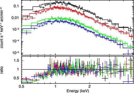
Spectra from rings 1 + 2 obtained on days 14.687, 16.857, 24.642 and 29.670 (ordered top to bottom). The spectra were jointly fit by an absorbed power law over the energy range 1–5 keV, then plotted down to 0.5 keV.
The dust scattering cross-section has an energy dependence of ∼E−2 over 1–5 keV (e.g. Draine 2003b). The dust spectrum should, therefore, be steeper than the incident spectrum by E−2, suggesting the spectrum of the flare responsible for the rings had a photon index of ∼2.5 (ranging from 2.3 to 2.8). This is significantly softer than the spectrum from the highest XRT flux interval from day 10.75 to 10.77 (see Section 3, below) which, together with the JEM X-1 low-energy light curve, provides further evidence that the final flare which formed the rings was a soft event.
3 MODELLING THE X-RAY SCATTERING FROM INTERSTELLAR DUST
If, like Mauche & Gorenstein (1986), we assume a silicate-like grain composition with a grain density ρ ≈ 3 g cm−3, then a typical grain radius a = 0.1 μm gives σscat ≈ 6.3 × 10⁻¹¹ cm2 at a photon energy of E = 1 keV. The projected geometric area of a grain is Ageom = πa2 so the ratio of the total cross-section to geometric cross-section is σscat/Ageom = 0.2 at 1 keV.
The geometry of the scattering applicable for V404 Cyg and the validity of the RG formulae are discussed in detail by Smith & Dwek (1998). Under the RG approximation it is assumed that the phase of the incident wave is not shifted by the dust medium and for sufficiently small scattering angles the waves scattered throughout a dust grain add coherently. Providing the numerical value of the X-ray energy in keV is significantly larger than the grain radius in μm, then the simple analytic form of the RG approximation is good. At lower energies or for larger grains the coherency assumption is broken and Mie scattering theory from spherical particles must be used (van de Hulst 1957); unlike the RG approximation, this cannot be reduced to a simple analytic form. The angular dependence of the differential cross-section from the Mie formulation is essentially the same as the RG approximation but for larger grains (or lower energies) its value is significantly reduced. At E = 0.5 keV and a = 0.4 μm, the differential scattering cross-section from the Mie calculation is a factor of ∼4.5 lower (Smith & Dwek 1998). Sharma (2015) recently identified a correction term which, when added to dσ/dΩ from the RG approximation, improves its agreement with the Mie calculation across a wider range of X-ray energies, whilst retaining an analytical approach. In addition to X-ray scattering, the Mie theory can also include absorption. For the grain sizes of interest and energies < 1 keV this further suppresses the differential scattering cross-section by a factor depending on the dust composition (i.e. density).
When modelling the dust scattering we only consider photon energies E > 1 keV, a dust density of |$3\ {\rm g\thinspace cm^{-3}}$| (silicate grains) and grain sizes ≲ 0.25 μm. For this range of parameters the dust differential scattering cross-sections predicted using the RG approximation are at most 5 per cent larger than those calculated using the full Mie scattering theory for spherical grains, while the angular dependence is the same (Smith & Dwek 1998; Corrales & Paerels 2015; Sharma 2015).
Unfortunately, we have no Swift-XRT coverage of the flare responsible for the rings, so use the inferred incident spectrum derived from the rings reported in Section 2.3 – i.e. a power law with photon index 2.5 (ranging from 2.3–2.8). The normalization of the (unabsorbed) power-law continuum was calculated from the 3–10 keV flux level (25 Crab) seen in the JEM X-1 light curve during the flare (assuming Crab spectral parameters from Kirsch et al. 2005), which for the photon index 2.5 case was approximately 420 photon cm− 2 s− 1 keV− 1 at 1 keV. These spectral parameters define F(E, t) and the outburst duration of 9160 s was used to specify the limits t1, t2.
Using equation (1), the fitted t0 and the delay times for each of the observations in Fig. 6, the observed radial profiles (in the energy range 1–4 keV), as a function of angle θ, were mapped into observed surface brightness profiles as a function of xD, where x ran from 0.20 to 0.95 in bins of width Δx = 0.005 and D = 2.39 kpc. Note, the lower usable x limit increases at later times as the higher θ angles fall outside the XRT field of view. Example remapped profiles are shown in Fig. 10. The bright rings associated with high dust density line up at the distances specified by the x values listed in Table 1, as expected. Equations (8)–(10) were used to fit all 21 profiles simultaneously, with model parameters a−/a+ = 0.1 (i.e. fixed to give a coverage of one decade over the power-law grain size distribution), a+, q, nd(x) (allowed to vary). The best-fitting values are listed in the first row of Table 2.
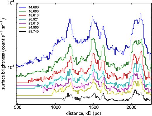
Representative observed halo surface brightness profiles, over the energy range 1–4 keV, resampled as a function of distance xD. The observation times (in days since the BAT trigger, 2015 June 15 18:31:38 ut) are shown in the legend and the profiles are offset vertically by 2.7 × 10³ Δt−0.75 for clarity (i.e. decreasing with time), where Δt is the time (in days) since the ring-forming flare.
Best-fitting grain model parameters for an F(E) = 421E−2.5 (photon cm− 2 s− 1 keV− 1) flare spectrum. Values in brackets indicate the 90 per cent confidence parameter ranges.
| Ring | x1Da | x2Db | a+c | qd | Nduste | |$\chi ^2_{\nu }$| | d.o.f |
|---|---|---|---|---|---|---|---|
| All | 484 | 2265 | 0.147 (0.143–0.171) | 3.90 (3.82–3.99) | 1.96 | 1.32 | 2532 |
| 955 | 1118 | 0.197 (0.165–0.288) | 4.26 (4.04–4.49) | 0.15 | 1.17 | 248 | |
| 5 | 1118 | 1251 | 0.150 (0.143–0.353) | 3.70 (3.54–3.95) | 0.29 | 1.22 | 218 |
| 4 | 1418 | 1580 | 0.268 (0.061–0.338) | 4.40 (4.01–4.80) | 0.07 | 1.18 | 258 |
| 3 | 1580 | 1689 | 0.309 (0.177–0.394) | 4.63 (3.61–5.53) | 0.22 | 1.32 | 178 |
| 2 | 1963 | 2083 | 0.165 (0.117–0.234) | 4.55 (4.06–5.02) | 0.19 | 1.01 | 198 |
| 1 | 2083 | 2202 | 0.208 (0.105–0.243) | 4.64 (3.97–5.36) | 0.10 | 1.10 | 178 |
Notes.aMinimum distance used in fit (pc); bmaximum distance used in fit (pc); cmaximum grain size (μm); dgrain size distribution index; edust column density (×1011 cm−2) integrated between x1 and x2.
Our results can be compared to those of Mauche & Gorenstein (1986), who modelled the haloes from a small sample of X-ray sources observed by the Einstein observatory. Our derived distribution index q ≈ 3.9 is within the range of values 3.5–4.5 they obtained, while our maximum grain size a+ ≈ 0.15 μm is just slightly smaller than theirs, which ranged from 0.2 to 0.3 μm. Likewise, our values are consistent with those of Predehl & Schmitt (1995), who studied the X-ray haloes around 25 sources observed during the ROSAT all sky survey and found an index q that ranged from 3.2–4.8 and maximum grain size a+ of 0.05–0.32 μm. Draine (2003b) noted that high q values and small maximum grain sizes fail to produce a sufficient quantity of large grains to model the standard ISM extinction law, which is better described by q ≈ 3.5 and a+ ≈ 0.25 μm, but is inconsistent with our results.
The fitted sampled array of the dust density profile, nd(xD), is shown in Fig. 11. The error bars were calculated from the rms scatter of the data-minus-model residuals in each x bin from the 21 profiles included in the fit, so represent approximate 1σ uncertainty estimates. As expected from Fig. 10, the profile reveals peaks in the dust density distribution at the distances inferred from the rings, with the highest density occurring at 1190 pc, associated with the closest dust sheet which forms the outer ring. The peak dust density is over ∼100 times larger than that typically found in the local ISM (e.g. Whittet 2003). The FWHM widths of the peaks correspond to dust sheet thicknesses of 40–80 pc.
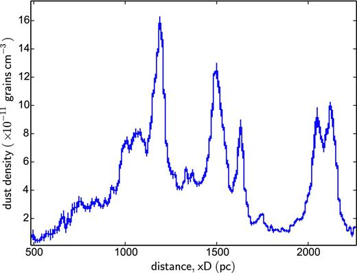
The fitted dust density profile, nd(xD), assuming an input source spectrum of 310 E− 2.3 photon cm− 2 s− 1 keV− 1 and grain size distribution n(a) ∝ a3.9 (with a maximum grain size a+ of 0.147 μm).
Integrating the density profile over distance gives a dust column density of Ndust ≈ 2 × 1011 cm−2. The uncertainty in the dust density distribution is dominated by the uncertainty in the normalization of the input source spectrum and its assumed spectral slope; different estimates of which are provided in Table 3. For example, a photon index of 2.3, which is the lower limit inferred from the spectral fits to the ring spectra (Section 2.3), scales the X-ray flux down by a factor of 1.25 and, hence, the dust density distribution up by the same amount, giving a total dust column of Ndust ≈ 2.5 × 1011 cm−2.
Dust column density and optical extinction estimates for different illuminating incident spectral models.
| Γa | FE(1 keV)b | Ndustc | |$\hat{E}{}^d$| | |$\hat{\sigma }_{\rm scat}{}^e$| | τscatf | AVg |
|---|---|---|---|---|---|---|
| 2.30 | 310 | 2.49 | 1.39 | 4.66 | 0.22 | 3.74 |
| 2.50 | 421 | 1.96 | 1.37 | 4.82 | 0.18 | 2.96 |
| 2.80 | 663 | 1.37 | 1.34 | 5.04 | 0.12 | 2.07 |
| Γa | FE(1 keV)b | Ndustc | |$\hat{E}{}^d$| | |$\hat{\sigma }_{\rm scat}{}^e$| | τscatf | AVg |
|---|---|---|---|---|---|---|
| 2.30 | 310 | 2.49 | 1.39 | 4.66 | 0.22 | 3.74 |
| 2.50 | 421 | 1.96 | 1.37 | 4.82 | 0.18 | 2.96 |
| 2.80 | 663 | 1.37 | 1.34 | 5.04 | 0.12 | 2.07 |
Notes.aSource spectrum photon index (E−Γ).
bSource spectrum normalization (photon cm− 2 s− 1 keV− 1) at 1 keV, required to give a flux of 25 Crab in the 3–10 keV band.
cIntegrated dust column density (×1011 cm−2).
dMean cross-section weighted photon energy over 1–4 keV.
eMean grain size weighted cross-section (×10−13 cm2).
fDust scattering optical depth at 1 keV, |$\tau _{\rm scat}=\hat{\sigma }_{\rm scat} N_{\rm dust} (\hat{E}/1{\rm keV})^2$|.
gOptical extinction (assuming τscat ≈ 0.06AV).
The sharp rise at 975 pc and other small well-defined peaks (e.g. at 1345 and 1740 pc) are indicative of genuine features in the dust density distribution, rather than artefacts produced by earlier flares, as the latter are spread out in x when the profiles are mapped with an incorrect flare time t0. While the profiles at early times do contain a low surface brightness background level caused by the previous flares, we estimate it contributes only ∼20 per cent of the low nd levels between the rings at 1830 pc (i.e. 2 × 10⁻¹² cm−3), or less than 5 per cent of the total column density.
The maximum grain size we find confirms the RG approximation is valid for the XRT data above 1 keV. Also, Mathis & Lee (1991) showed that multiply scattered photons start to dominate over single scatterings when τscat > 1.3. Our modelling suggests τscat < 0.22 for V404 Cyg and hence multiple scatterings are not important in the energy band we have considered. Use of the full Mie theory would give the same angular dependence as the RG approximation and hence similar values for the fits to the grain size distribution would be obtained. The Mie scattering cross-sections are around 5 per cent lower than those obtained by the RG approximation, therefore, the best-fitting dust column densities would be correspondingly larger, but essentially the same given the uncertainties are dominated by the choice of input spectrum used in the modelling.
VP15 used a different approach and modelled the integrated scattered flux from rings 1 + 2, 3 + 4 and 5, but allowed the grain size distribution to vary between the rings. They found an index q ranging from 3.5 for rings 3 + 4 to 4.4 for rings 1 + 2 and maximum best-fitting grain sizes from 0.17–0.24 μm (though the latter values were not well constrained for rings 1 + 2 and 5).
In order to test for variations in the dust distribution parameters between the rings we have also fit the main features from the profiles in Fig. 10 independently, the results of which are included in Table 2. While we see a factor of 2 variations in the best-fitting maximum grain size values (e.g. ring 3 compared with ring 5), they agree within the uncertainties. On the other hand, ring 5 shows a significantly shallower grain size distribution index of q ≈ 3.7 compared with some of the other rings, indicating that the grain size distributions could indeed be different between the dust scattering regions along the line of sight. The grain size distributions we derive are consistent with VP15 for rings 1, 2 and 5, but our fits require a steeper index q for rings 3 and 4 (with the latter pair dominated by ring 4). We find the dust sheet responsible for the nearest ring has the highest column density, as was also the case for the modelling approach which assumed an average dust grain size distribution across all rings. This differs from the results of VP15, who found the column density was greatest for the ring 3 + 4 pair.
Comparison of the column density estimates calculated over the rings (listed in Table 2) with the corresponding values from Fig. 11, reveal Ndust changes by factors of ∼0.5–2.7 when the parameters a+ and q are allowed to vary; for example, Ndust is a factor of 1.8 larger for ring 3 and 2.7 smaller for ring 4, which would invert their respective peak heights shown in Fig. 11. The overall integrated column density along the line of sight is reduced by approximately 25 per cent.
The azimuthal profiles (Fig. 8) revealed significant variations in the dust scattering emission as a function of angle around the central source, with differences seen from one ring to another. Such variations indicate there are significant changes in the dust density distribution perpendicular to the line of sight, which could in principle be used to map the 3D distribution of dust.
4 DISCUSSION
Dust scattering rings were seen in X-ray observations of V404 Cyg obtained by the Swift-XRT during its 2015 June outburst. A radial profile analysis reveals five bright rings, as well as other lower intensity emission, which expand and fade with time. By fitting the expected θ ∝ t1/2 angular evolution of the rings we find they were formed by a bright X-ray flare from the central black hole binary that occurred at 2015 Jun 26 16:54 ut, with an uncertainty of 39 min. INTEGRAL JEM X-1 data confirmed the presence of flaring activity at this time, which corresponded to the brightest recorded event from the entire outburst, reaching a flux of approximately 25 Crab in the 3–10 keV band.
Given the distance to V404 Cyg is known from parallax measurements (2.39 ± 0.14 kpc; Miller-Jones et al. 2009), then the locations of the density enhancements in the ISM responsible for producing the rings were obtained from the fits to their angular evolution and were found to be at distances of 1187 ± 70, 1505 ± 88, 1630 ± 95, 2050 ± 120 and 2127 ± 125 pc, where the uncertainties are dominated by the error on the central source distance.
The dust scattered X-ray spectrum observed from the rings over 1–5 keV was found to be very steep, with a photon index Γ ∼ 4.5. As the dust scattering cross-section has an E−2 energy dependence above 1 keV, this implies the incident flare spectrum (which was not observed by the XRT) should be soft, with a photon index of ∼2.5. This is significantly softer than that seen from XRT observations of the central source taken during flaring intervals earlier in the outburst.
Detailed radial profile modelling assuming the dust grain density ng(a, x) can be separated out as n(a)nd(x), where n(a) ∝ a−q is a power-law distribution of grain sizes a and nd(x) is the dust density profile as a function of fractional distance x, allows the latter to be recovered. We find the average dust properties are well modelled by a grain size distribution index |$q = 3.90^{+0.09}_{-0.08}$| and a maximum grain size a+ of |$0.147^{+0.024}_{-0.004} {\rm \ \mu m}$|.
The derived dust density distribution shows five peaks, one for each of the dust sheets responsible for the rings, with the maximum density occurring at the location of the nearest sheet to the Earth. An integrated dust column density of Ndust ≈ (2.0–2.5) × 1011 cm−2 is found to be consistent with the optical extinction to V404 Cyg.
4.1 The location of V404 Cyg
Figs 12 and 13 highlight the position of V404 Cyg in the surrounding Galactic environment. Fig. 12 is a schematic plan view of the Galaxy with the locations of V404 Cyg, the Sun and various high-mass star-forming regions (HMSFRs) from the Bar and Spiral Structure Legacy (BeSSeL) and VLBI Exploration of Radio Astrometry maser surveys (Reid et al. 2014) marked. As viewed from the Earth, V404 Cyg lies along the direction of the Local Arm, which is thought to be a significant structure of the Galaxy, situated between the Perseus and Sagittarius spiral arms (e.g. Xu et al. 2013).
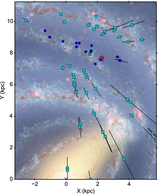
Schematic view of the Galaxy illustrating the position of V404 Cyg (red star), the Sun (⊙) and a number of HMSFRs in the Local Arm (blue hexagons) and other spiral arms (cyan squares) obtained from the BeSSeL survey (see text). The HMSFR G074.03−01.71 is marked with a green triangle. (Galaxy image credit: R. Hurt, NASA/JPL-Caltech/SSC.)
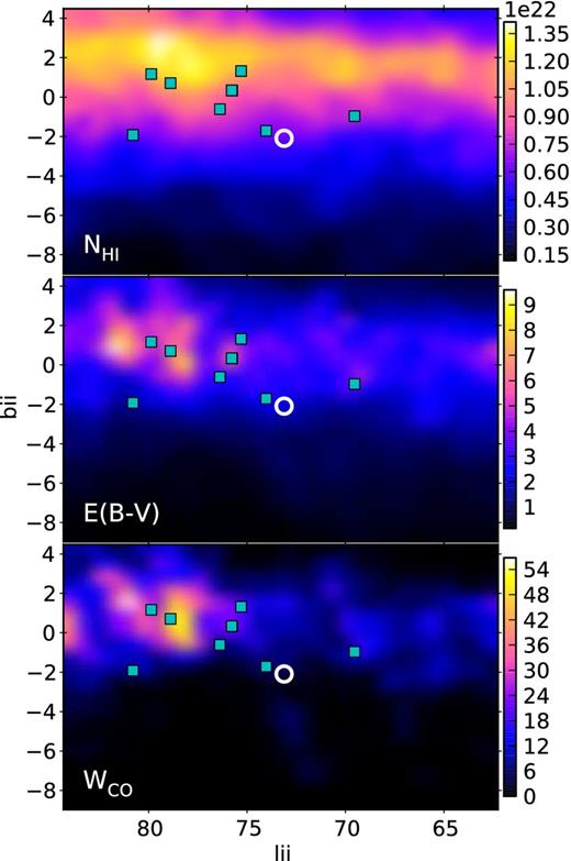
Sky maps illustrating the distribution of absorbing material in the vicinity of V404 Cyg. The upper panel shows the integrated atomic hydrogen column density (|${\rm N_{{\rm H}\,{\small {i}}}}$|, units cm−2) from the LAB 21 cm survey (Kalberla et al. 2005). The middle panel shows the Galactic reddening (E(B − V), mag) derived from 100 μm emission (Schlegel et al. 1998). The bottom panel shows the CO emission map (WCO, in K km s−1) of Dame et al. (2001). In each panel, the position of V404 Cyg is marked by a white circle, while cyan squares show the locations of Local Arm HMSFRs from the BeSSeL survey.
The Local Arm maser sources are also marked on Fig. 13, which shows the location of V404 Cyg with respect to the neutral hydrogen column density distribution from the Leiden/Argentine/Bonn (LAB) 21 cm survey (Kalberla et al. 2005, upper panel), the interstellar reddening map derived from IRAS and COBE/DIRBE IR observations (Schlegel, Finkbeiner & Davis 1998, middle panel) and the Millimeter-Wave Telescope CO Survey emission at 115 GHz (Dame, Hartmann & Thaddeus 2001, lower panel). The latter, which is often used to trace molecular hydrogen in dense molecular clouds (e.g. Glover & Mac Low 2011), was found to correlate with the dust-to-hydrogen ratio by Willingale et al. (2013). The bright area in the CO map near l, b = 79°, 0° corresponds to the Cygnus X region, which is one of the largest and most active star formation regions in the Galaxy at a distance of 1.7 kpc (Schneider et al. 2006).
V404 Cyg is situated at a Galactic latitude of −2.09 deg, which, at a distance of 2.39 kpc, places it 87 pc below the Galactic plane. Fig. 13 shows that at this latitude, the column density and extinction start to increase significantly towards the plane. The LAB neutral hydrogen (H i) column density in the direction of V404 Cyg is |$N_{\rm H\,\small {i}} = 6.65\times 10^{21}{\rm \ cm}^{-2}$|, while the Schlegel et al. (1998) extinction map gives an E(B − V) ≈ 1.9 (i.e. AV ≈ 5.9, assuming an extinction to reddening ratio RV = 3.1),4 implying an additional column from molecular hydrogen of |$2N_{\rm H_2}=1.44\times 10^{21}{\rm \ cm}^{-2}$| (Willingale et al. 2013), giving a total column density of NH, tot = 8.1 × 1021 cm−2.
While this superficially agrees with the column derived from the spectral fits to the rings (Section 2.3) and central source, the H i column density estimate is obtained by integrating the LAB 21 cm data over all velocities along the line of sight (i.e. through the Galaxy), which includes material in the Perseus and Outer spiral arms that are more distant than V404 Cyg. Examination of the 21 cm radial velocity data reveals that these structures could account for ∼30–50 per cent of the H i column along this sight line, implying the total column should be significantly lower. However, the observed X-ray column (≈8 × 1021 cm−2) suggests that either our line of sight soon exits the Galactic plane, in which case any additional contribution to the H i column from behind the source would be minimal, or local variations in column exist on angular scales smaller than the resolution available in the LAB map (0.675 deg).
The measured visual extinction of V404 Cyg of AV ≈ 4 (Hynes et al. 2009) is also lower than the line of sight inferred extinction estimates of Schlegel et al. (1998) or Schlafly & Finkbeiner (2011), which is to be expected given the relatively nearby location of the source. The optical extinction to column density relation of Predehl & Schmitt (1995), AV/NH(1021 cm−2) ≈ 0.56, predicts a neutral hydrogen column density of (7.1 ± 0.8) × 1021 cm−2 for the observed visual extinction range of V404 Cyg (AV = 3.6–4.4; Hynes et al. 2009), in agreement with the LAB 21 cm estimate. The equivalent relationship from Valencic & Smith (2015) gives column densities which are 17 per cent higher.
One of the HMSFR masers, G074.03−01.71, is at an angular separation of just 0.99 deg from V404 Cyg and has a parallax derived distance of 1.59 ± 0.04 kpc (Xu et al. 2013). This places it at a distance consistent with that obtained from the ISM dust density enhancements responsible for rings 3 or 4, indicating they may be spatially connected, with the dust sheet extending at least 28 pc at right angles to the line of sight.
4.2 CO and IR maps in the vicinity of V404 Cyg
Fig. 14 shows an expanded view of the CO map of Dame et al. (2001) centred on V404 Cyg (resolution of 7.5 arcmin). The image was created from the low radial velocity data |VR| < 10 km s−1 to exclude any contributions to the CO emission from behind V404 Cyg, such as the Perseus spiral arm. CO emission is used as a proxy for tracing H2 in molecular clouds, though it does not necessarily correlate well with dust, as when carbon is locked up in molecules it is then not available to form grains. The strongest feature in the CO map, which contains the HMSFR G074.03−01.71 at its northern end, occurs at an angular distance ≳ 30 arcmin from V404 Cyg – i.e. much further out than the rings seen by the XRT. The CO emission is relatively weak at the location of V404 Cyg, measuring 3.3 K km−1, which using the CO-to-H2 conversion factor of 2 × 1020 cm−2 K−1 km from Bolatto, Wolfire & Leroy (2013), implies a molecular hydrogen column density of |$2 N_{\rm H_2} = 1.32\times 10^{21}{\rm \ cm}^{-2}$|, similar to the estimate from Willingale et al. (2013) noted above. The CO emission varies by less than ∼50 per cent within 10 arcmin of the source.
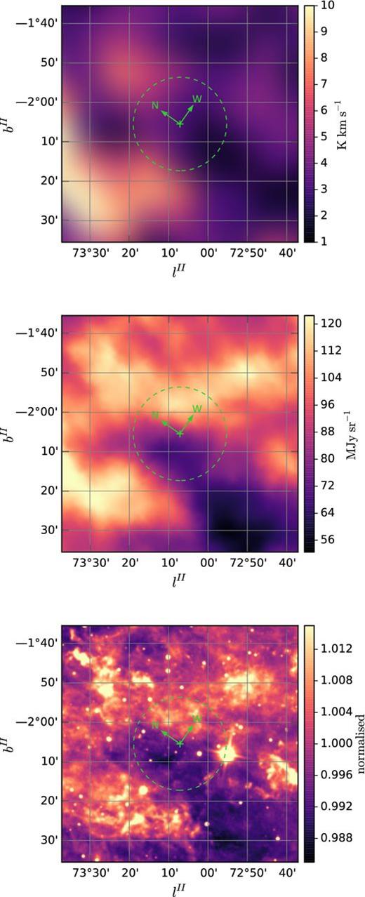
Galactic coordinate maps centred on V404 Cyg in different wavebands : (top) CO 115 GHz emission (resolution 7.5 arcmin); (middle) IRAS 100 μm emission (resolution 4.3 arcmin); (bottom) WISE 22 μm emission (resolution 12 arcsec). The dashed circle shows the size of XRT field of view (11.8 arcmin radius). The arrows identify the equatorial coordinate west (azimuthal angle ϕ = 0°) and north (ϕ = 90°) directions.
One of the most reliable way to map the distribution of dust is via its far-IR emission, which at 100 μm is dominated by the thermal emission from larger grains (a ≳ 0.01 μm; e.g. Draine 2003a). Fig. 14 also shows the IRAS 100 μm emission map from the improved survey reprocessing (Miville-Deschênes & Lagache 2005)5, which has a resolution of 4.3 arcmin. The 100 μm map reveals 50 per cent variations in IR emission on sub-10 arcmin angular scales at the location of the source, with the brightest IR emission occurring on its Galactic north side.
It is noticeable that there is reduced IR emission within 10 arcmin of V404 Cyg on its Galactic south-east side. This is the equatorial east direction and corresponds to angles of ϕ ∼ 170°–210° in the azimuthal profiles of Fig. 8, where minima in the profiles are seen.
The Wide-field Infrared Survey Explorer (WISE; Wright et al. 2010) satellite observed V404 cyg at mid-IR wavelengths during its all-sky survey in 2010. The 22 μm image, at a resolution of 12 arcsec, from the NASA/IPAC Infrared Science Archive6 is also shown in Fig. 14. While point sources have not been removed from the image, the diffuse mid-IR emission is still readily apparent, with few per cent variations occurring on arcminute scales. At 22 μm, emission from smaller silicate grains (a ≲ 0.01 μm) becomes important, while a significant contribution from carbonaceous grains in the form of polycyclic aromatic hydrocarbons (PAHs) is also to be expected (Draine 2003a).
The 22 μm image confirms the overall large-scale brightening in the diffuse IR emission in the Galactic north direction (i.e. equatorial azimuthal angle ϕ ∼ 340°–360°, 0°–80°), noted in the lower resolution far-IR image above, as well as subarcminute structure. Surface brightness profiles created from the mid-IR image show the flux increases by 1 per cent over an angular distance of ∼1–3 arcmin from the source towards the Galactic north, followed by a similar but slower rise out to a radius of 7 arcmin, before it starts to decline. A decline in mid-IR flux by a comparable amount is seen in profiles away from the source in the equatorial east/south-east direction (ϕ ∼ 170–210) out to ∼7–9 arcmin, confirming the reduction in the diffuse IR emission that was apparent in the lower resolution far-IR image. This direction coincides with the minima seen in the XRT azimuthal profiles from the rings.
4.3 X-ray rings and IR emission compared
Fig. 15 shows a comparison of the expansion of the rings as seen by the XRT with the WISE 22 μm emission – the latter plotted as contours. Note, in the online version of the paper, the figure is animated and steps through different XRT images when opened with the Adobe Reader PDF viewer and the primary mouse button is pressed. Other viewers may not support the animation. In this equatorial projection, Galactic north and the trend of increasing IR emission occurs in the north-west direction (ϕ ∼ 35°).

Representative XRT images (in equatorial coordinates) showing the evolution of the rings, along with the WISE 22 μm data plotted as contours (at normalized levels of 0.9885, 0.9940, 0.9995, 1.0050 and 1.0105 from dark-grey to white). The XRT data were smoothed by convolving with a Gaussian of width σ = 7.1 arcsec. The mid-point observation times of the XRT data are marked in the upper-left corner of each image. The arrows in the top right identify the Galactic coordinate north and west directions. Note, the azimuthal angle ϕ = 0° direction points towards the west (i.e. right). The XRT image is animated in the online version of this paper.
At first glance, the X-ray azimuthal profile variations apparent in Figs 8 and 15 do not appear to be well correlated with the diffuse emission structure seen in the mid-IR data. For example, the maxima in the X-ray azimuthal variations from rings 3 and 4 (ϕ ∼ 120°–130°) occur at right angles to the direction of the overall brightening seen in the mid-IR flux levels. Whilst the northernmost maximum seen in the X-ray azimuthal variations from ring 5 coincides with the largest IR flux increase (at an azimuthal angle of ϕ ∼ 70° and radius of ∼6–7 arcmin), the southern component (which peaks near an azimuthal angle ϕ ∼ 270°) shows no equivalent large scale rise in the IR flux level. However, the X-ray emission from the innermost ring, which is also brighter in the equatorial south (ϕ ∼ 270°), may be associated with a slight increase in the diffuse IR emission levels between radii of ∼2–5 arcmin in this direction.
It is noticeable that the X-ray emission from ring 2 most obviously tracks the general increase in IR flux towards Galactic north, as might be expected if the higher IR flux was caused by an increase in dust density in this direction. For example, ring 2's X-ray azimuthal profile relative brightness increases from day 16.690 at ϕ ∼ 350°,7 which, at a radius ≳ 2.5 arcmin, coincides with the direction where the mid-IR emission level rises by just over 1 per cent in 4 arcmin. This suggests that at least some of the increase in IR emission on the Galactic north side of the source might be associated with the dust sheet responsible for ring 2 at a distance of 2.05 kpc.
Despite this, it might seem surprising that we do not see a somewhat more significant correlation between the IR emission maps and the X-ray scattering azimuthal variations. However, IR observations of star-forming regions in different wavebands reveal that dust emission consists of separate components with distinct spatial distributions – for example, at 20 μm, emission from PAHs and smaller grains ( ≲ 0.01 μm) dominate and are associated with the most intense radiation fields around the youngest SFRs, whereas at 100 μm, emission from a more diffuse component associated with larger grains ( ≳ 0.01 μm) is seen (e.g. Kennicutt & Evans 2012). Therefore, the lack of significant 22 μm counterparts to the X-ray azimuthal variations might suggest the spatial distribution of large grains responsible for the X-ray scattering is also different to that of the smaller grains which gives rise to the majority of the mid-IR emission.
Furthermore, since the IR emission from dust is powered by the absorption of starlight, then the spatial distribution of stellar sources is also important in shaping the observed IR emission properties and not just the spatial distribution of the dust – the latter is, therefore, more reliably probed by the X-ray scattering observations.
Both X-ray scattering and far-IR emission are expected to originate from a population of grains with sizes larger than 0.01 μm. Unfortunately, the angular resolution of the 100 μm map is too low (4.3 arcmin) to be able to explore the relationship between any far-IR variations and the X-ray scattering from the rings in great detail, though on large scales, both the far-IR and X-ray data show a reduction in their respective flux levels in the equatorial east/south-east direction.
As the IR map is composed of the integrated flux from the different layers along the line of sight, it would be difficult to interpret the true spatial dependence of the dust from the IR emission alone. On the other hand, the X-ray observations of the rings allowed the dust density profile to be estimated, as well as the azimuthal variations to be characterized, and provide the clearest view of the ISM dust properties in the direction of V404 Cyg.
5 SUMMARY
We have analysed Swift-XRT data taken during the recent outburst from V404 Cyg. The XRT images show the clearest example of dust scattering rings from any X-ray transient source to date, with five distinct components visible in the radial profiles. The angular evolution of the rings allow the time of the flare responsible for their formation to be pin-pointed and it was found to be temporally coincident with the largest flare seen by INTEGRAL's JEM X-1 instrument, which peaked at 25 Crab in the 3–10 keV band.
Detailed modelling of the radial profiles, employing the RG approximation for the dust scattering cross-section, allowed us to quantify the dust properties. Assuming a power-law distribution of grain sizes, ∝ a−q, we found the dust emission was best fitted by q ≈ 3.9, with a maximum grain size a of 0.15 μm.
The dust density profile along the line of sight was also estimated, with the densest layers responsible for the rings located at distances of 1187 ± 70, 1505 ± 88, 1630 ± 95, 2050 ± 120 and 2127 ± 125 pc from the Earth. The width of the density profile peaks imply dust sheet thicknesses ranging from 40–80 pc. The maximum density of dust grains occurs at the position of the sheet nearest to Earth (1.19 kpc). An integrated dust grain column density of Ndust ≈ (2.0–2.5) × 1011 cm−2 was found to agree with the optical AV = 3.6–4.4 to the source.
An archival WISE 22 μm image reveals diffuse mid-IR emission variations within 10 arcmin of the source. Comparing the evolution of the rings over the same angular scales suggests the second most distant ring follows the general mid-IR emission trend, which exhibits an increase in flux on the Galactic north side of the source. Azimuthal profiles of the X-ray emission around the rings show a minimum towards the Galactic south-east, coinciding with a reduction in IR flux in this direction.
We also note that the HMSFR G074.03−01.71 is less than a degree away from V404 Cyg and has a parallax derived distance which places it at a distance comparable to that of rings 3 or 4, suggesting the regions might be spatially connected.
We thank the Swift and INTEGRAL teams for graciously granting, then performing the observations, as well as the numerous ToO requesters who asked for observing time. APB, JPO and KLP acknowledge support from the UK Space Agency. GRS acknowledges support from an NSERC Discovery Grant. APB thanks the authors of the excellent python, numpy, scipy, matplotlib, nlopt and astropy software, which were used during this work. We thank the referee whose comments helped improve the manuscript.
This research has made use of the NASA/IPAC Infrared Science Archive, which is operated by the Jet Propulsion Laboratory, California Institute of Technology, under contract with the National Aeronautics and Space Administration.
NOTE ADDED IN PRESS
Heinz et al. (2016) recently published an independent analysis of the X-ray dust scattering rings seen around V404 Cyg, using both Chandra and Swift data. They derive a dust distribution along the line of sight to the source similar to the one found here.
The initial BAT trigger time, which corresponds to MJD 57188.772 (UTC), is used as a zero-point reference time throughout this paper.
Note, D was fixed in the fitting procedure as D and x are highly correlated parameters.
Note, the linear structures extending across the X-ray images on days 14.687 and 16.690 are caused by a reduction in exposure due to the unfortunate positioning of the XRT CCD bad-columns during these observations.
REFERENCES
