


Abstract
This paper is the second in a pair of papers presenting data release 1 (DR1) of the Herschel Astrophysical Terahertz Large Area Survey (H-ATLAS), the largest single open-time key project carried out with the HerschelSpace Observatory. The H-ATLAS is a wide-area imaging survey carried out in five photometric bands at 100, 160, 250, 350 and 500 μm covering a total area of 600 deg2. In this paper, we describe the identification of optical counterparts to submillimetre sources in DR1, comprising an area of 161 deg2 over three equatorial fields of roughly 12 × 4.5 deg centred at 9h, 12h and 14|${^{\rm h}_{.}}$|5, respectively. Of all the H-ATLAS fields, the equatorial regions benefit from the greatest overlap with current multi-wavelength surveys spanning ultraviolet (UV) to mid-infrared regimes, as well as extensive spectroscopic coverage. We use a likelihood ratio technique to identify Sloan Digital Sky Survey counterparts at r < 22.4 for 250-μm-selected sources detected at ≥4σ (≈28 mJy). We find ‘reliable’ counterparts (reliability R ≥ 0.8) for 44 835 sources (39 per cent), with an estimated completeness of 73.0 per cent and contamination rate of 4.7 per cent. Using redshifts and multi-wavelength photometry from GAMA and other public catalogues, we show that H-ATLAS-selected galaxies at z < 0.5 span a wide range of optical colours, total infrared (IR) luminosities and IR/UV ratios, with no strong disposition towards mid-IR-classified active galactic nuclei in comparison with optical selection. The data described herein, together with all maps and catalogues described in the companion paper, are available from the H-ATLAS website at www.h-atlas.org.
1 INTRODUCTION
The Herschel Astrophysical Terahertz Large Area Survey (H-ATLAS; Eales et al. 2010) is the largest area submillimetre (submm) survey conducted with the HerschelSpace Observatory (Pilbratt et al. 2010), imaging around 600 deg2 at 100 and 160 μm with PACS (Poglitsch et al. 2010) and 250, 350 and 500 μm with SPIRE (Griffin et al. 2010), as described by Ibar et al. (2010), Pascale et al. (2011) and Valiante et al. (2016, hereafter Paper I). Data release 1 (DR1) covers 161 deg2 in three equatorial fields at RA of approximately 9h, 12h and 14|${^{\rm h}_{.}}$|5 (GAMA9, GAMA12, GAMA15), and benefits from extensive multi-wavelength coverage in the Sloan Digital Sky Survey (SDSS; York et al. 2000), the Galaxy Evolution Explorer (GALEX; Martin et al. 2005), the UK Infrared Deep Sky Survey Large Area Survey (UKIDSS-LAS; Lawrence et al. 2007), the Wide-field Infrared Survey Explorer (WISE; Wright et al. 2010), the VISTA Kilo-degree Infrared Galaxy Survey (VIKING; Edge et al. 2013) and the VST Kilo-Degree Survey (KiDS; de Jong et al. 2013). These fields are especially valuable due to the extensive supporting data and analysis provided by the Galaxy And Mass Assembly (GAMA) survey (Driver et al. 2011), including highly complete spectroscopic redshifts (Liske et al. 2015) and matched-aperture photometry from far-ultraviolet (FUV) to submm (Driver et al. 2016).
In order to unlock the scientific capabilities of these rich data sets, one of the first challenges is to identify counterparts across the various surveys, a problem of particular difficulty in the submm due to poor angular resolution and the relatively flat redshift distribution of sources in contrast with other wavebands. A popular approach to this problem is the likelihood ratio (LR) technique (Richter 1975; Sutherland & Saunders 1992; Ciliegi et al. 2003), which was adopted for the identification of SDSS counterparts in the H-ATLAS science demonstration phase (SDP) by Smith et al. (2011, hereafter S11), Spitzer-IRAC counterparts in SDP by Kim et al. (2012), VIKING counterparts in the DR1 GAMA9 field by Fleuren et al. (2012) and WISE counterparts in GAMA15 by Bond et al. (2012).
In this paper, we apply the LR technique to H-ATLAS DR1 to find counterparts in SDSS DR7 (Abazajian et al. 2009) and DR9 (Ahn et al. 2012), using additional data from UKIDSS-LAS and GAMA. For counterparts within the GAMA main survey (primarily r < 19.8), we take advantage of matched FUV-to-mid-IR photometry provided by GAMA, combining data from SDSS, GALEX, VIKING and WISE (Driver et al. 2016). We use the results to determine the multi-wavelength properties and physical nature of 250-μm-detected sources above ∼30 mJy, including magnitude distributions, optical/infrared (IR) colours, redshift distribution and IR luminosities. Throughout the paper, we quote magnitudes in the AB system unless otherwise stated, and assume a cosmology with |$\Omega _\Lambda =0.73$|, ΩM = 0.27 and H0 = 71 km s−1 Mpc−1.
2 DATA
2.1 Submillimetre catalogues
We use the H-ATLAS DR1 source catalogues described in Paper I, which are extracted from the 250 μm maps using MADX (Maddox, in preparation) with a matched-filter technique (Chapin et al. 2011) to minimize instrumental and confusion noise. The source catalogues used for matching contain 37 612, 36 906 and 39 472 sources detected with 250 μm signal-to-noise ratio (SNR) ≥4 in the GAMA9, GAMA12 and GAMA15 fields, respectively. The 4σ detection limit is 24 mJy for a point source in the deepest regions of the maps (where tiles overlap), or 29 mJy for a point source in the non-overlapping regions (the average 4σ point source detection has S250 = 27.8 mJy). The catalogues also contain a small fraction of sources selected at 350 or 500 μm, which have 250 μm SNR <4. We exclude these from this analysis because their red submm colours indicate a high redshift, and any identification with an SDSS source is likely to be false, resulting from either chance alignment or lensing (Negrello et al. 2010; Pearson et al. 2013).
For the LR calculations, we treat all 250 μm detections as point sources (see Section 3.2) but for the discussion of multi-wavelength properties in Section 6, we use the best flux measurement for each source in each band, as described in Paper I.
2.2 Optical catalogues and classifications
2.2.1 Sample selection
We opt to search for counterparts in SDSS because this is currently the deepest comprehensive survey of the full DR1 sky area. We use all primary objects in SDSS DR7 with rmodel < 22.4 (see Table 1 for numbers). We use DR7 because, unlike later releases, it contains size information that is used for identifying H-ATLAS sources requiring extended flux measurements. We found that 163 and 433 additional objects were present in DR9 (in GAMA9 and GAMA12, respectively), close to bright stars that were masked in DR7. These sources were added to our optical catalogue to maximize the completeness. We cleaned the catalogue by removing a total of 3749 spurious objects, which are generally either galaxies which have been deblended into multiple primary objects (for example where a spiral arm or bright region has been identified as a separate object from the galaxy) or stars with diffraction spikes which are detected as multiple objects. These cases were identified by visually inspecting all SDSS objects with r < 19 that had deblend flags and were within 10 arcsec of a SPIRE source; in each case, only the brightest central object was retained in the cleaned catalogue (see also S11). The total of 3749 also includes spurious objects identified by performing a self-match on SDSS coordinates with a search radius of 1 arcsec, since these close pairs are always the result of incorrect deblending in the SDSS catalogue rather than genuine pairs of separate sources.
2.2.2 Redshifts
Spectroscopic redshifts (zs) were obtained from the GAMA II redshift catalogue (SpecCat v27), which is close to 100 per cent complete for r < 19.8 (Liske et al. 2015). In addition to GAMA redshifts from the Anglo-Australian Observatory (AAO) and Liverpool Telescope (LT), we include redshifts collected from SDSS DR7 and DR10 (both galaxy and QSO targets; Ahn et al. 2013), WiggleZ (Drinkwater et al. 2010), 2SLAQ-LRG (Cannon et al. 2006), 2SLAQ-QSO (Croom et al. 2009), 6dFGS (Jones et al. 2009), MGC (Driver et al. 2005), 2QZ (Croom et al. 2004), 2dFGRS (Colless et al. 2001), UZC (Falco et al. 1999) and NED.1 The GAMA redshifts cover two samples, the main sample and the filler sample. The main sample is based on SDSS galaxy selection to rpetro < 19.8 primarily. In addition to these, H-ATLAS-selected galaxies were added as filler targets from 2011 February. Filler targets were selected for H-ATLAS sources with reliable optical counterparts (reliability R > 0.8), that were part of the GAMA input catalogue (selected from SDSS with rpetro < 20.0 or rmodel < 20.6). In addition, the same masking and star–galaxy separation were applied to select the filler sample as per the GAMA main sample (Baldry et al. 2010). Redshifts were considered reliable if they had quality nQ ≥ 3. The main sample is highly complete with over 98 per cent meeting this criterion, while 86 per cent of the H-ATLAS fillers were observed spectroscopically with 63 per cent having nQ ≥ 3. Completeness at r ≳ 20 is lower, although the SDSS DR10 and WiggleZ surveys provide a considerable contribution here (see also Section 5.1). We discarded GAMA redshifts with low quality (nQ < 3) and SDSS redshifts with any spectroscopic flags set. For objects with redshifts in multiple surveys, we favoured the one with the highest quality flag, and where this was not possible we selected in order of preference (i) GAMA, (ii) SDSS DR10, (iii) WiggleZ, (iv) other surveys. The distribution and origins of redshifts in our final catalogue are described in more detail in Section 5.1.
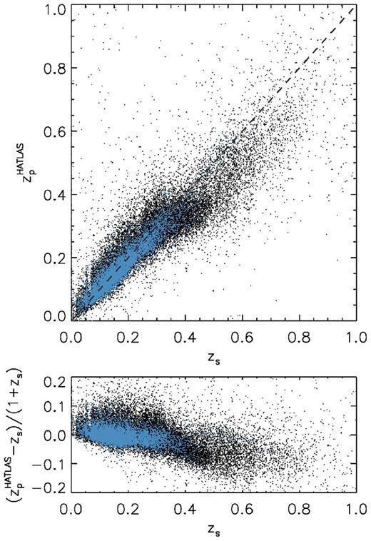
The optical catalogues also contain photometric redshifts measured from the SDSS ugriz and UKIDSS YJHK photometry for all candidates in our optical catalogue, although these are not used for the LR analysis. The photometric redshifts are described in detail in S11. They were estimated by empirical regression using the neural network technique of annz (Collister & Lahav 2004), by constructing a training set of spectroscopic redshifts from GAMA I (Driver et al. 2011), SDSS DR7, 2SLAQ, AEGIS (Davis et al. 2007) and zCOSMOS (Lilly et al. 2007), which covers magnitudes r < 23 (with >1000 galaxies per unit magnitude) and redshifts z < 1 (with >1000 in each Δz=0.1 bin). In Fig. 1, we analyse the accuracy of these photometric redshifts, and compare them against those from the SDSS (DR7/DR9) Photoz table.2 The annz redshifts show less bias and smaller scatter than the SDSS ones, showing the benefit of including near-IR photometry from UKIDSS.
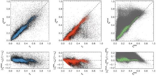
Left: comparison of the H-ATLAS photometric redshifts (zp from ugrizYJHK) and available spectroscopic redshifts (zs). Black points show the zp of all galaxies with a zs, and blue show the subset with measurement errors Δzp/(1 + zp) < 0.02. Middle: comparison of the SDSS photometric redshifts (from ugriz) and available spectroscopic redshifts. Black points show the zp of all galaxies with a zs and red show the subset with measurement errors Δzp/(1 + zp) < 0.02. Right: direct comparison of the H-ATLAS and SDSS photometric redshifts. Grey points show all data with both zp measurement errors Δzp/(1 + zp) < 0.1, and green show those with both zp measurement errors Δzp/(1 + zp) < 0.02. The lower panels show the respective fractional deviations in zp. To reduce crowding, we plot only one quarter of available data in each panel.
2.2.3 Separating stars, galaxies and quasars
Star–galaxy separation was carried out using similar constraints to S11 and the GAMA input catalogue (Baldry et al. 2010). Specifically, galaxies were defined as objects satisfying any of the following constraints, indicating that they are either extended or have colours inconsistent with stars:
Δsg > 0.25 and not zs < 0.001;
Δsg > 0.05 and Δsgjk > 0.40 and not zs < 0.001;
Δsg > fsg and not zs < 0.001;
GAMA Kron ellipse defined and not zs < 0.001.
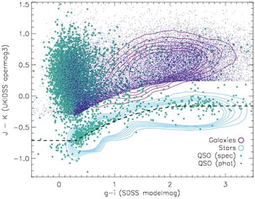
Star–galaxy separation using SDSS and UKIDSS colours. The dashed line given by equation (3) describes the sequence of stars. Galaxies (magenta contours) are separated from stars (blue contours) using the criteria described in Section 2.2.3, based on redshift and size information as well as the colours. Quasars are identified as unresolved objects with spectroscopic redshifts >0.001 (turquoise circles), and this sample is supplemented with candidate quasars (blue points) which are unresolved objects with non-star-like colours but no secure spectroscopic redshift available.
Quasars (QSOs) were identified as SDSS objects which do not satisfy any of the criteria (i–iv) above (i.e. unresolved in the r band and with non-stellar colours), and which have secure spectroscopic redshifts z > 0.001. We also classified as quasars all objects which had been classified as quasars by their SDSS spectra, defined by the criteria class=‘QSO’ and zwarning=0 in the SpecObj table of SDSS DR12. In addition to these ‘spectroscopic’ QSOs, we identified photometric QSO candidates as objects which do not satisfy (i–iv), have no spectroscopic redshift, but have Δsgjk > 0.40 (i.e. non-stellar colour). The numerical results of each classification are shown in Table 1.
Statistics of SDSS candidates within the SPIRE masks of the three fields.
| Sample | GAMA9 | GAMA12 | GAMA15 |
|---|---|---|---|
| SPIRE SNR250 ≥ 4 | 37 612 | 36 906 | 39 479 |
| Mask area (deg2) | 53.42 | 53.47 | 54.53 |
| SDSS rmodel < 22.4 | 1127 518 | 976 822 | 1105 073 |
| After cleaning | 1126 510 | 975 630 | 1103 891 |
| Stars | 540 739 | 365 708 | 488 648 |
| Galaxies | 754 598 | 603 327 | 603 578 |
| QSOs (spectroscopic) | 3545 | 2921 | 5769 |
| QSOs (photometric) | 7628 | 3674 | 5896 |
| Spectroscopic redshifts | 66 368 | 72 868 | 81 464 |
| H-ATLAS zp | 1107 539 | 963 395 | 1092 258 |
3 LR ANALYSIS
The identification of counterparts (‘IDs’) to submm sources can be tackled in a statistical way using the LR technique to assign a probability (‘reliability’) to each potential match, and thus distinguish robust counterparts from chance alignments with background sources. The LR method relies on knowledge of the intrinsic positional uncertainty of the sources as well as the magnitude distributions of true counterparts and background sources. When the sample size is sufficiently large, it is preferable to divide the matching catalogue into different source classifications to measure these statistics for each class of object (Sutherland & Saunders 1992; Chapin et al. 2011, S11; Fleuren et al. 2012). We therefore calculate magnitude statistics separately for stars and for extragalactic objects (galaxies and QSOs, both spectroscopic and photometric). We assume that positional errors are independent of the source classification, but we take into account the potential bias for redder submm sources that was highlighted by Bourne et al. (2014), as we shall describe in Section 3.2.
3.1 Magnitude distributions
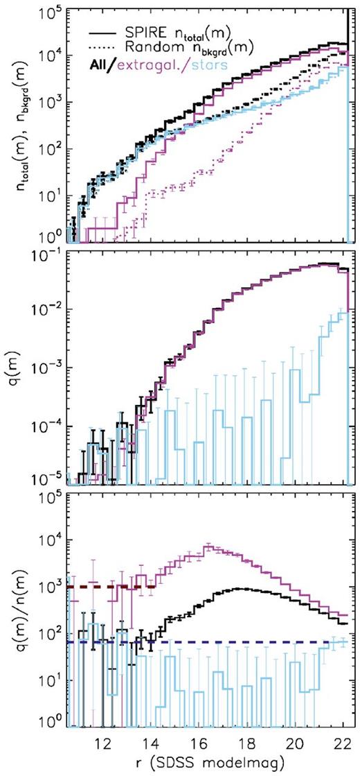
The method of measuring the r-band magnitude distribution of true counterparts. Top panel: magnitude distribution of SDSS objects within 10 arcsec of all SPIRE positions (solid lines) divided into galaxies and quasars (magenta) and stars (blue), and the total (heavy black line). The background magnitude distributions of SDSS (normalized to the same search area) are given by the dashed lines (the background distribution of stars closely follows that of SPIRE centres). Middle panel: the magnitude distribution of true counterparts q(m) is given by the difference between SPIRE and random distributions above, normalized to Q0. Bottom panel: the ratio of the magnitude distribution of true counterparts to that of background objects is used in the calculation of LR in equation (5). At magnitudes m < 14.0 (galaxies) and m < 21.5 (stars), the value of q(m)/n(m) is fixed at the average within this range, as shown by the horizontal dashed lines.
3.1.1 The normalization Q0
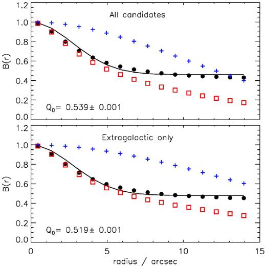
The method of measuring the fraction of SPIRE sources without counterparts (1 − Q0) by counting ‘blanks’ (objects with no candidate within the search radius) as a function of the search radius. Red squares show the blank counts centred on real SPIRE positions, blue crosses show the blank counts around random positions and black circles show the ratio. The black line is the best fit to the black circles using the model described by equation (7). Top panel: all optical candidates; bottom panel: galaxies and quasars only.
We can show this by instead calibrating Q0 from the normalization of the magnitude histograms (as in S11), giving Q0 = 0.616 for galaxies, suggesting that the level of bias from clustering and multiple sources is significant. A further independent measurement can be obtained from the normalization of the positional offset histograms (see Section 3.2). This measurement is Q0 = 0.548 ± 0.009 for galaxies, which accounts for clustering via a cross-correlation term but can still be boosted by multiple counterparts, unlike the blanks method. Comparing the various methods, we might suggest that Q0 can be boosted by 0.03 due to multiplicity, and by a further 0.07 due to clustering, although these estimates are rough and dependent on the models assumed (for example the power-law correlation function assumed in Section 3.2). We will discuss the sensitivity of the results to the value of Q0 in Section 4.4.
Field-to-field variance is also likely to be significant between the 16 deg2 SDP field and the 161 deg2 in DR1, and this probably accounts for the different measurements for stars. The three GAMA fields sample quite different Galactic latitudes and hence sightlines through the disc and halo of the Milky Way: GAMA9 is at b = +28, GAMA12 is at b = +60 and GAMA15 is at b = +54. The standard deviation in Q0 from the blanks method between the three DR1 fields (each ≈53 deg2) is 0.011 for galaxies and 0.011 for stars.
3.1.2 Application to the LRs
We take the difference between the SPIRE-centred and background magnitude histograms, nreal(m), and normalize this to Q0 to give q(m), as shown in the middle panel of Fig. 3. In calculating the LR for extragalactic candidates, we use the measured q(m)/n(m) distribution for r-band magnitudes m > 14.0, but at brighter magnitudes the distribution is not well sampled and we assume a constant q(m)/n(m) equal to the average of q(m)/n(m) at m < 14.0. The same method is used for stellar candidates, except that the threshold must be set at m = 21.5 because there are too few to measure the magnitude distributions at m < 21.5. The measured distributions of q(m)/n(m) are shown by the histograms on the lower panel of Fig. 3, while the constant values adopted for bright magnitudes are indicated by the horizontal dashed lines. In this respect, our method differs from S11, who assumed a constant q(m) for stars [as opposed to constant q(m)/n(m)], which would lead to a higher LR for brighter stars compared with fainter ones since n(m) rises towards fainter magnitudes. Our assumption of flat q(m)/n(m) at m < 21.5 instead leads stars to have an LR independent of magnitude. Our motivations for this choice are (i) that the use of a constant q(m) [hence non-constant q(m)/n(m)] at m < 21.5 would lead to a discontinuity in the lower panel of Fig. 3 where the decreasing q(m)/n(m) at increasing m meets the measurements at m > 21.5 which are relatively high, and (ii) that we do not necessarily expect any correspondence between optical magnitude and the detectability of a star at 250 μm.
This last point deserves some explanation. The submm emission associated with stars is likely to come from debris discs or dust in outflows and so may not be directly related to the photospheric optical luminosity. We might still expect a correlation between optical and submm fluxes because the dust emission in these systems is simply reprocessed starlight, and also because the flux in both wavebands depends on distance. However, there is a large amount of scatter in the masses and temperatures of debris discs around stars of a given spectral type (Hillenbrand et al. 2008; Carpenter et al. 2009), and H-ATLAS will detect only the brightest of these (Thompson et al. 2010). The statistics of H-ATLAS-detected stars will therefore be highly stochastic, and any correlation between submm detectability and optical magnitude is likely to be broken. The effect of this assumption on LR statistics is discussed in Section 4.5.
Finally, in Section 4.2 we visually check the positions of bright stars to ensure that none are missing from the ID catalogue. We find that the few bright stars detected at 250 μm are successfully identified by the LR procedure, and none of them are missing from the SDSS catalogue. This indicates that the measured q(m) for bright stars is not underestimated due to incompleteness of SDSS at bright magnitudes.
3.2 Positional offset distributions
The final ingredient for measuring the LR of each potential counterpart is the probability that a real counterpart is found at the measured radial separation r from the SPIRE source. For the purposes of assigning LRs to counterparts, we make the simplifying assumption that all H-ATLAS sources are point-like in the 250 μm maps from which they were extracted, with a beam full width at half-maximum of 18.1 arcsec. This assumption is justified by the fact that a maximum of 2 per cent of the sources are resolved,4 and that these will be galaxies at z < 0.05 with bright, unambiguous SDSS counterparts.
The random background of chance alignments, which is effectively constant across the histogram since the probability of chance alignment is equal in any given sightline.
True SDSS counterparts, which exist for a fraction Q0 of all SPIRE sources, and whose distribution follows the positional error function f(r).
Nearby SDSS objects that are physically correlated with the SPIRE source (due to galaxy clustering), but are not direct IDs, whose distribution is given by the cross-correlation between the SPIRE and SDSS samples, governed by a power law w(r) convolved with f(r).
3.2.1 Measuring the cross-correlation
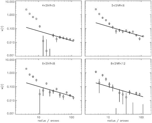
Cross-correlations between the SPIRE 250 μm positions in bins of SNR and the SDSS positions across the three fields. Error bars represent Poisson counting errors. The power-law fits shown include only the data at r > 10 arcsec in order to remove any bias from the true counterparts which are at smaller radii. In these fits, the slopes are fixed to −0.7 and the best-fitting normalization parameters are given in Table 2.
Best-fitting parameters in modelling SDSS positional offsets to blue SPIRE sources with S250/S350 > 2.4 in bins of 250 μm SNR.
| SNR | NSPIRE | r0/arcseca | σpos/arcsecb, c | Q0 b |
|---|---|---|---|---|
| 4–5 | 2990 | 0.20 ± 0.02 | 2.38 ± 0.02 | 0.792 ± 0.008 |
| 5–6 | 1435 | 0.61 ± 0.05 | 1.91 ± 0.02 | 0.846 ± 0.010 |
| 6–8 | 1316 | 0.38 ± 0.05 | 1.59 ± 0.01 | 0.944 ± 0.008 |
| 8–12 | 776 | 0.38 ± 0.08 | 1.19 ± 0.01 | 0.985 ± 0.008 |
3.2.2 Measuring the positional errors
Finally, we fit the two-dimensional histograms of ΔRA and ΔDec. separations with the model in equation (11), fixing w(r) with the power-law parameters described above, and solving for the widths (σpos, RA, σpos, Dec.) of the Gaussian f(r), the background level n0 and the normalization Q0. We do this in each of the SNR bins, using only blue sources with S250/S350 > 2.4, to avoid the lensing-related biases discussed in Bourne et al. (2014) and in Section 3.2 above. The fitting is performed on the two-dimensional histograms, and in Fig. 6 we show the histograms and best-fitting models collapsed along the ΔRA and ΔDec. axes for visual inspection. The fitting results are summarized in Table 2. Note that the normalization (Q0) fitted to these histograms differs from the results in Section 3.1.1 because it depends on both SPIRE colour and SNR, but this normalization can also be boosted by the existence of multiple counterparts. We will investigate the dependence of our ID results on the measurement of Q0 in Section 4.4.
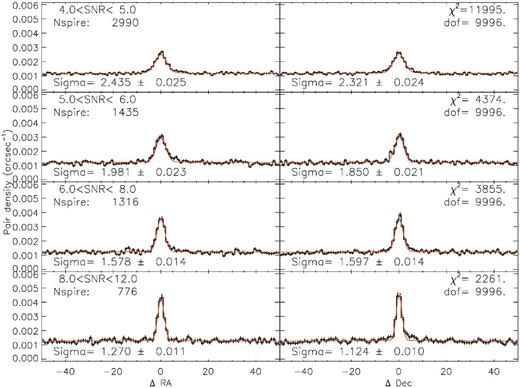
The two-dimensional histograms of positional offsets between SPIRE sources in the blue bin (S250/S350 > 2.4), and all SDSS candidates within ±50 arcsec in RA and Dec. are shown collapsed along the RA and Dec. axes (left and right, respectively), divided into bins of SPIRE SNR (from top to bottom). The orange line shows the best-fitting model given by equation (11) with the widths σpos (arcsec) and the χ2 and degrees of freedom (dof) printed in the respective panels.
Bourne et al. (2014) showed the colour dependence of the width σpos by dividing the sample into six bins of colour and four of SNR. We repeat this analysis on the matched-filter catalogues used here and show the best-fitting σpos values in each bin in Fig. 7. In this analysis, the bluest colour bin contains the results shown in Fig. 6. The increasing σpos and weakening SNR dependence in redder colour bins demonstrates the bias which is likely due to lensing, and the need to measure the true value of σpos using blue SPIRE sources only.

Dependence of the positional error on SPIRE SNR and colour. Top panels: the best-fitting σpos values (RA, Dec., and the geometric mean thereof) from the two-dimensional offset histograms, as a function of SPIRE SNR, for sources in six bins of 250/350 μm colour. The bluest bin is the data plotted in Fig. 6. Bottom: the same data plotted as a function of colour in the four SNR bins. The dotted lines show the best-fitting power-law models for σpos as a function of SNR in each colour bin (top panels), and as a function of colour in each SNR bin (bottom panels).
3.2.3 Robustness of the positional errors
The positional error for a 5σ source given above (2.10 ± 0.01 arcsec) differs from the value of 2.40 ± 0.09 arcsec used in the SDP (S11) for the following reasons: first S11 measured σpos for all sources with SNR>5, rather than binning by SNR and colour, which would lead them to measure a larger overall σpos due to the bias from red sources as discussed above. Additionally, the use of a matched filter in the DR1 source extraction has improved the positional accuracy compared with the PSF-filtering used in SDP (Paper I), and this reduces the measured σpos. We validated our σpos measurement by using the same flux cut as S11 on catalogues made from PSF-filtered DR1 maps, with no SNR/colour binning, and found a value of σpos = 2.39 arcsec, consistent with 2.40 arcsec in S11.
It is apparent in Fig. 5 that there is the potential for degeneracy between the parameters of the cross-correlation (which dominates radial separations on large scales) and those of the positional error (which dominates on small scales). To test what effect the fit to the cross-correlation has on the fit for σpos, we compare the results given by fitting the cross-correlation on different scales. The results given above were obtained from a cross-correlation fit with a slope of δ = −0.7 on scales r > 10 arcsec. If we fit the cross-correlation to scales of r > 5 arcsec, we obtain a slope of −1.9 (r0 = 5.23 arcsec) and the resulting change in the fit for the positional error with this alternative w(r) is such that σpos is reduced by a factor 0.91, and f(r) and L would therefore be boosted by a factor 0.97. We therefore conclude that our results are not strongly affected by the choice of correlation function assumed.
4 RESULTS
4.1 LRs and reliabilities
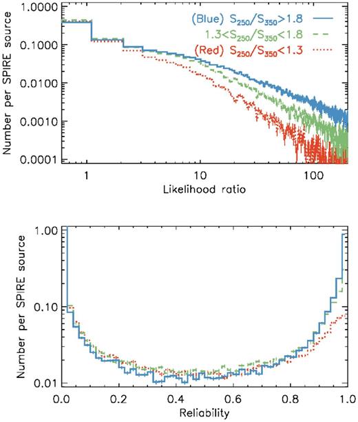
LRs and reliabilities of H-ATLAS sources in bins of 250/350 μm colour.
4.2 Catalogue checks and flags
The LR procedure relies on the assumptions that SPIRE sources are unresolved at 250 μm, that the optical positions and magnitudes are precisely known, and that the optical catalogue is complete. These assumptions break down in a minority of cases. Large, nearby galaxies are resolved in the SPIRE image so the positional error on the SPIRE source does not follow f(r), and the positional error of the optical centroid is also non-negligible. Furthermore, the optical magnitude can be unreliable due to limitations in the automated SDSS photometry especially in the case of clumpy star-forming discs or discs with dust lanes, and clumpy galaxies or bright stars can be broken up into multiple sources in SDSS.5 The LR and reliability results can underestimate the true reliability of a cross-match in such cases. It is also unavoidable that optical IDs are missed due to incompleteness in the optical catalogues, especially where SDSS catalogues are masked close to bright stars.
While we cannot realistically hope to correct all such failures in the catalogue, we should at least ensure that no bright SPIRE sources are missing IDs that would be easily identifiable by eye. We therefore visually inspected the brightest 300 SPIRE sources in each of the three fields, and flagged objects with missing optical counterparts, with misclassified optical counterparts, or where the reliability was underestimated for resolved SPIRE sources or for galaxy mergers. We also visually inspected all SPIRE sources within 10 arcsec of a star in the Tycho catalogue, to ensure that no bright stellar IDs were missing from SDSS, and found that none were missing. A total of 13 missing IDs were added as a result of visual inspection, taking data from the NED, GAMA and SDSS. We also modified the reliabilities of 65 IDs which had been underestimated by the automated procedure (resolved galaxies and mergers), changed the galaxy/star classification of 40 bright objects that had been misclassified (mostly bright stars with saturated optical photometry), and removed 28 optical counterparts that were found to be artefacts or duplicates resulting from the breaking up of large galaxies or bright stars in the SDSS catalogue (in general, these had not been given high reliability, but occasionally they affected the reliability of the true counterpart). Since all of these problems are associated with bright objects, we are confident that their effect on the IDs of fainter sources that were not inspected is small or negligible. In addition to those visually inspected, we searched SDSS DR8 for any matches within 10 arcsec of SPIRE sources with no potential counterpart in the original optical catalogue (leading to 1105 additional optical candidates, all of which were visually confirmed).6 The LR and reliability values were re-calculated for all potential counterparts to SPIRE sources affected by these additions. The numbers in Table 3 reflect these changes, but they are not included in the input samples described in Table 1.
Results of ID analysis by field.
| H-ATLAS sample | GAMA9 | GAMA12 | GAMA15 | Total |
|---|---|---|---|---|
| SPIRE SNR250 ≥ 4 | 37 612 | 36 906 | 39 479 | 113 997 |
| SDSS candidates ≤10 arcsec | 42 770 | 40 462 | 44 898 | 128 130 |
| Reliable IDs (R ≥ 0.8) | 14 280 | 14 900 | 15 655 | 44 835 |
| Stars | 95 | 224 | 103 | 422 |
| Galaxies | 13 864 | 14 389 | 15 199 | 43 452 |
| QSOs (spectroscopic) | 159 | 203 | 248 | 610 |
| QSOs (photometric) | 162 | 84 | 105 | 351 |
| Spec-z | 7422 | 7727 | 8589 | 23 738 |
| GAMA FUV detections | 3618 | 4089 | 4698 | 12 405 |
| GAMA NUV detections | 5344 | 5543 | 6449 | 17 336 |
| GAMA r detections | 7472 | 7655 | 8371 | 23 498 |
| GAMA K detections | 7494 | 7669 | 8381 | 23 544 |
| GAMA W1 detections | 7168 | 7457 | 8116 | 22 741 |
| GAMA W4 detections | 1587 | 1963 | 2786 | 6336 |
4.3 ‘Reliable’ IDs: completeness and contamination
Details of the IDs in each field are listed in Table 3. As in S11, we choose to define ‘reliable’ counterparts as all matches with R ≥ 0.8, in order to select a sample which is both very clean (minimizing false counterparts) and dominated by sources with low blending. This latter result is due to the Li values on the denominator of equation (16). For example, if a close pair of galaxies with similar magnitudes are found at equal distances from the submm centroid, and both have very high LRs (L1 ≈ L2 ≫ 1 − Q0), either galaxy could be identified as a likely counterpart. However, the high LR of each one reduces the reliability of the other since the ratio L1/(L1 + L2) ≈ 0.5 ensures that the reliability of each is not greater than 0.5. Thus, a cut of R ≥ 0.8 is biased against potentially interacting galaxies, including blended submm sources as well as interacting systems where only one object is a submm source; on the other hand, it leads to well-matched fluxes for spectral energy distribution (SED) fitting (S11, 2012).
We can assess the effect of changing the reliability cut by measuring the completeness and cleanness of the ‘reliable’ sample as a function of the threshold, as shown in Fig. 9. The chosen cut of R ≥ 0.8 selects a very clean sample at the expense of completeness. Any increase in the cut would lead to a sharp fall in completeness, although a lower cut could be used to increase completeness with a modest drop in cleanness. However, it is not possible to get close to 100 per cent completeness without a cut of around 0.5 or less, and such a cut would lead to complications in the analysis since a one-to-one matching between SPIRE and optical counterparts would not be guaranteed. Note that 100 per cent completeness would mean that the fraction of sources with reliable IDs is equal to Q0, not unity.
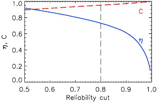
The effect of changing the reliability cut on the ‘reliable’ sample's completeness η (blue solid line), given by equation (18), and cleanness (red dashed line), given by C = 1 − Nfalse/NSPIRE. The vertical dashed line indicates the cut used to define the ‘reliable’ sample in this and other H-ATLAS papers. In principle, any value can be chosen for this cut to suit the needs of a given project.
We have chosen to use the cut of R ≥ 0.8 for our analysis, but the data release contains the full set of potential counterparts with likelihood and reliability data for each, so users are free to make their own decision on this issue.
4.4 Sensitivity to the value of Q0
Our assumption of a universal constant Q0 may lead to inaccuracies for certain subsets of sources since the fraction of real IDs which appear in SDSS will be a function of redshift, hence will vary with both submm flux and colour. In Section 3.2, we estimated Q0 from the SPIRE–SDSS positional offset histograms for blue (S250/S350 > 2.4) SPIRE sources in SNR bins, and found higher Q0 for the blue sources, increasing with SNR (Table 2). Although these values could be slightly biased by multiplicity of counterparts, we can use them to test the sensitivity of the LR results to Q0. The advantages of using this blue subset are that it is unlikely to contain a significant lensed population which could bias Q0, and that it is likely to have the largest deviation from the average Q0, since the majority of the sources will be at low enough redshifts to appear in SDSS. The average Q0 for blue SPIRE sources and galaxy/QSO candidates in SDSS is 0.858 (the number-weighted average of values in Table 2).
We re-calculated the LR for the 13 992 blue SPIRE sources using Q0 = 0.858 for extragalactic objects (keeping Q0 = 0.020 for stars unchanged, on the assumption that their Q0 is independent of SPIRE colour), and compared the results to the release catalogue which was processed using Q0 = 0.519 for extragalactic objects. The release catalogue contains reliable IDs for 10 320 of the 13 992 blue SPIRE sources, but using the higher Q0 leads to an additional 708 IDs, or 5.1 per cent of the blue SPIRE sources. If we assume that the true value of Q0 for this subset is 0.858 + 0.020, then equation (18) indicates that the completeness of IDs for blue sources in the release catalogue is 84 per cent, but this would rise to 90 per cent if we were to include the additional 708 IDs.
Extending this analysis to the whole population of SPIRE IDs is not straightforward, but our underestimate of Q0 is certain to be greatest in this blue SPIRE bin; hence, overall statistics will be affected less significantly than the results above indicate. Q0 for the reddest sources will be lower than the average (they are at higher redshift and less likely to appear in SDSS), and the bias shown above is likely to be reversed for that subset. However, we cannot reliably measure Q0 for red sources unless we can account for the bias from lensed sources which are falsely identified with the foreground lensing system in SDSS. For this reason, we have used the overall estimate of Q0 in our release catalogue. A more ideal solution would be to measure Q0 as a function of SPIRE flux and colour, accounting for the bias from lensing, but we leave this extension to the method for future work.
4.5 Sensitivity of stellar counterparts
In Section 3.1.2, we described a change in the method used for calculating the LR of stellar counterparts, by assuming a constant q(m)/n(m) instead of a constant q(m) (as in S11), thereby discarding the assumption of a link between optical magnitude and detection in the submm. Our motivation for this choice was based on the high measured q(m)/n(m) at faint magnitudes and the weakness of the presumed link between optical and submm brightness. The effect of this decision is significant for the statistics of stellar IDs. By assuming higher q(m)/n(m) at faint m, we boost the LRs of the majority of stars, at the expense of the few bright stars, and this in turn leads to higher reliabilities and an overall count of 422 reliable stellar IDs. For comparison, the flat-q(m) method employed in SDP (S11) would lead to only 161 reliable stellar IDs in DR1. This also impacts on the galaxy IDs, because their reliabilities depend on the LRs of all potential counterparts including stars, and so our method yields 188 fewer reliable galaxy IDs than the flat-q(m) method. The completeness and contamination fractions of galaxy IDs do not change significantly, but the estimated completeness of stars is higher using our new method (η = 18.1 per cent versus 7.1 per cent), although the contamination from false IDs is also higher (14.9 per cent versus 10.3 per cent) – see equations (17) and (18). Furthermore, the number of stellar IDs in common between the two methods is only 41, meaning that the reliability of stellar counterparts is highly dependent on the assumptions made about q(m). Since we cannot measure this at m < 21.5, it is not necessarily true that our new method is an improvement on the SDP method, although it is consistent with the data that we have for q(m); hence, the reliabilities of stellar IDs must be taken with a degree of caution (as previously noted by S11).
A further degree of uncertainty arises from the fact that the relatively high q(m) measured for stars at m > 21.5 (see Fig. 3, middle panel) may be biased by misclassification of faint galaxies as stars based on SDSS imaging. If this contamination of the stars is significant, then we may have overestimated the LRs of stellar counterparts [due to overestimating q(m)/n(m)], while those misclassified galaxies will have their LR underestimated [since galaxies have higher q(m)/n(m)]. This issue can only be resolved with further investigation of the statistical properties of submm-bright stars.
In spite of these uncertainties, there are likely to be many more stars detected in H-ATLAS than the reliable sample would suggest (as indicated by the low completeness), although the LR process has failed to identify unambiguously which sources they are, owing to inadequate prior knowledge of the magnitude distribution of 250-μm-detected stars. This situation could perhaps be improved by stacking analyses or prior-based ‘forced photometry’ on known star positions, or an analysis of the Herschel debris disc surveys DUNES (Eiroa et al. 2010) and DEBRIS (Matthews et al. 2010). We leave such improvements for future work.
4.6 The incidence of multiple counterparts
The disadvantage of the reliability metric is that it assumes that each SPIRE source has a single counterpart, although this counterpart may not be detected in the optical survey. This means that the reliability of a given match can be inaccurate if the SPIRE source is a blend of two or more galaxies, all of which could be treated as genuine counterparts. The bias against interacting systems (mentioned in Section 4.3) is especially relevant since many bright far-IR (FIR) sources are known to be interacting (e.g. Bettoni, Mazzei & Della Valle 2012).
It is difficult to reliably estimate the fraction of SPIRE sources which have multiple genuine counterparts. One can start by comparing the results of using the LR instead of the reliability to define counterparts (S11), since the LR contains no information on the existence of other potential counterparts but simply gives the ratio of the probability of a single potential match to that of a chance alignment. In the cases where there is only one potential ID, equation (16) implies that an LR of 1.924 corresponds to the threshold R = 0.8 for galaxy matches (Q0 = 0.519). Hence, to avoid the effects of multiplicity on the reliable IDs, we could apply this LR cut and find 50 421 extragalactic IDs, of which 6539 (13.0 per cent) fail the R ≥ 0.8 threshold. These additional IDs could be considered candidates for sources with multiple counterparts which have been missed by the reliability cut, although in reality these will be a mixture of true multiples (mergers, pairs and close groups) as well as chance alignments where the single true counterpart is ambiguous.
An alternative approach is to suggest that multiple counterparts are missed by the requirement for a single match to have R ≥ 0.8, but can be recovered by assuming that the sum of their reliabilities meets this threshold (Fleuren et al. 2012). In DR1, 3483 SPIRE sources have multiple extragalactic counterparts whose ∑R ≥ 0.8, but for which no single counterpart meets the threshold. This estimate for the missed multiple counterparts is smaller than that from the LR threshold (6539), because there will be systems where multiple low-reliability (but high-LR) counterparts do not have a high combined reliability. Following Fleuren et al. (2012), we can further clean this list of candidate multiple counterparts by selecting only those with spectroscopic redshifts which agree within 5 per cent, or photometric redshifts within 10 per cent, in order to exclude chance alignments. This requirement reduces the number to 2071 SPIRE sources with multiple extragalactic counterparts at the same redshift. This is a small fraction of the total number of reliable IDs, so we can conclude that most SPIRE sources in H-ATLAS have single galaxy IDs.7
A related issue is the incompleteness of the sample due to multiplicity, which results from the fact that additional candidates in the search radius reduce the reliability of the true counterpart. Fleuren et al. (2012) estimated this incompleteness by comparing the fraction of reliable IDs among all SPIRE sources with one candidate, those with two candidates, and so on. In Table 4, we show these fractions for SPIRE 250 μm sources with between 0 and 10 candidates, including either all candidates or only extragalactic ones. For example, 49 057 SPIRE sources have only one potential counterpart within 10 arcsec from the full optical catalogue, and of these 52 per cent are reliable IDs; 24 194 have two potential counterparts but of these 58 per cent are reliable, suggesting that sources are more likely to be assigned an ID if there are two candidates in the search radius. The fraction of reliable counterparts then falls for increasing numbers of potential candidates. Looking at extragalactic candidates only, the fraction of reliable counterparts is 61 per cent when there is only one candidate, and this fraction falls when more candidates are available. One might ask why the fall was not seen when counting all candidates, and we suggest that the reason is that the reliable fraction of sources with only one candidate ID is depressed by the fact that a disproportionate number of stellar IDs fall in this bin (stars tend to be isolated), and their reliabilities are generally lower.
Number of SPIRE sources and the subset of those with reliable IDs, as a function of the number (p) of candidate IDs within the 10 arcsec search radius [counting either all candidates or extragalactic (xgal) candidates only].
| With p candidates: | With p xgal candidates: | |||
|---|---|---|---|---|
| p | NSPIRE | Nrel (per cent) | NSPIRE | Nrel (per cent) |
| 0 | 31 394 | 0 (0) | 41 142 | 0 (0) |
| 1 | 49 057 | 25 648 (52) | 49 898 | 30 669 (61) |
| 2 | 24 194 | 14 026 (58) | 18 013 | 11 043 (61) |
| 3 | 7365 | 4075 (55) | 4109 | 2245 (55) |
| 4 | 1661 | 897 (54) | 722 | 366 (51) |
| 5 | 280 | 123 (44) | 96 | 41 (43) |
| 6 | 39 | 18 (46) | 12 | 5 (42) |
| 7 | 4 | 2 (50) | 2 | 1 (50) |
| 8 | 3 | 1 (33) | 3 | 1 (33) |
| 9 | 0 | 0 (–) | 0 | 0 (–) |
The falling reliable fraction with increased number of extragalactic candidates can be interpreted as incompleteness resulting from multiplicity. We can estimate this by adding up the total number of missing ‘reliable’ counterparts from each row of the table, assuming that in each case the intrinsic number is 61 per cent of NSPIRE, and the result is 408 missing IDs. Hence, we conclude that the incompleteness of IDs resulting from multiplicity is small.
5 OPTICAL PROPERTIES OF H-ATLAS IDS IN SDSS
In this section, we explore the properties of H-ATLAS sources with ‘reliable’ optical counterparts, using optical photometry from SDSS and redshifts from the sources described in Section 2.2.2.
5.1 Redshifts and magnitudes
Fig. 10 shows the relationship between optical magnitude of all reliable SDSS counterparts, 250 μm flux and redshift (for extragalactic counterparts). The 250 μm flux is weakly correlated with redshift, in contrast with the optical magnitude which is a strong function of redshift; this is a result of the differential k-corrections. Almost all of the bright sources in H-ATLAS with S250 ≳ 200 mJy are at z < 0.1, but at lower fluxes, sources are detected at all redshifts up to z ∼ 0.7 and the upper limit in the redshift distribution is clearly a result of the depth of SDSS rather than that of H-ATLAS.
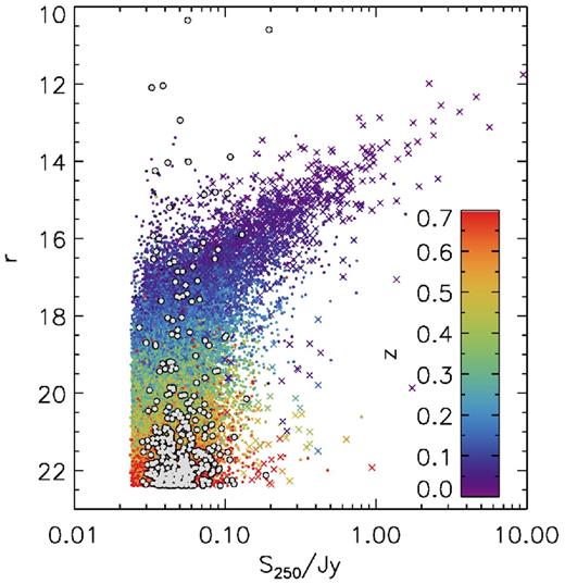
Optical magnitudes in the r band versus 250 μm fluxes of H-ATLAS sources with reliable IDs in SDSS. Extragalactic sources are coloured according to their redshift (spectroscopic where available; photometric otherwise). Stars are shown by grey circles. For most sources, we plot the point source flux at 250 μm, which is the flux measurement used to define the 4σ sample. However, for a relatively small number of extended sources at low redshifts (plotted as crosses), we plot the aperture flux as described in Paper I, where this exceeds the measured point source flux.
Stellar counterparts, shown by grey circles in Fig. 10, exhibit no correlation between their optical and submm fluxes. As discussed in Section 3.1.2, we do not necessarily expect a correlation between the optical and submm fluxes of the stars we can detect, although we note that the increased number of stellar IDs towards fainter optical magnitudes r ≳ 21 may be a cause for concern. It is likely that the optical classification of stars is more uncertain close to the r-band limit, and that more galaxies are misclassified as stars. If the large number of stellar IDs at r ≳ 21 in Fig. 10 are in fact misclassified galaxies, this may indicate a larger number of such misclassifications in the optical catalogue, and since the Q0 for stars is much lower than that for galaxies, these objects are much less likely to have been assigned reliable IDs. Hence, the completeness of galaxy IDs at faint r-band magnitudes may be adversely affected. In fact, we can estimate how bad this problem could be by looking at the completeness as a function of magnitude estimated first from all possible counterparts, and secondly from only those potential counterparts that we have classified as extragalactic (we describe how this is measured in Section 5.2). The completeness at r > 21 falls by roughly 0.05 between these two samples (at brighter magnitudes it does not change significantly). This means that even if all the star classifications at r > 21 are false, and should be galaxies, then our completeness is only about 5 per cent worse than it should be at these faint magnitudes. On the other hand, the contamination of stellar IDs by unresolved galaxies could be significant (as mentioned in Section 4.5), and optical imaging at higher resolution (compared with typical SDSS seeing of 1.5 arcsec) is needed to confirm these.
Approximately half (49 per cent) of reliable IDs have a spectroscopic redshift, while the overall fraction of all potential counterparts in the catalogue which have spectroscopic redshifts is 21 per cent. These redshifts originate primarily from GAMA (69 per cent) and SDSS DR7/DR10 (24 per cent); the full breakdown of all redshifts (not only reliable IDs) is shown in Table 5. 2583 of the 22 808 spectroscopic redshifts from GAMA were obtained within the H-ATLAS filler programme (as described in Section 2.2.2).
Number of good quality (nQ ≥ 3) redshifts in the full ID catalogue originating from each survey.
| Survey | Reference | Number |
|---|---|---|
| GAMA-AAO | Liske et al. (2015) | 22 804 |
| GAMA-LT | Liske et al. (2015) | 4 |
| SDSS DR7 | Abazajian et al. (2009) | 5811 |
| SDSS DR10 | Ahn et al. (2013) | 2424 |
| WiggleZ | Drinkwater et al. (2010) | 1226 |
| 2dFGRS | Colless et al. (2001) | 777 |
| MGC | Driver et al. (2005) | 211 |
| 2QZ | Croom et al. (2004) | 142 |
| 2SLAQ-QSO | Croom et al. (2009) | 117 |
| 2SLAQ-LRG | Cannon et al. (2006) | 59 |
| 6dFGS | Jones et al. (2009) | 21 |
| NED | http://ned.ipac.caltech.edu/ | 3 |
| UZC | Falco et al. (1999) | 2 |
| Total | 33 601 |
The overall redshift distribution of H-ATLAS sources is shown in the upper panel of Fig. 11, in comparison with that of GAMA. Our use of spectroscopic redshifts from SDSS DR10 and WiggleZ makes up for the lack of redshifts for faint galaxies in GAMA, and photometric redshifts fill in any remaining gaps. The fact that almost all reliable counterparts at z > 1 have spectroscopic redshifts may be explained by those objects being specifically targeted by BOSS (Eisenstein et al. 2011), but it could also be affected by a bias in photometric redshifts. The potential bias arises from a tendency of the annz code to return solutions at zp < 1 because this range is best represented in the training set. Note that Fig. 11 only describes the redshift distribution of 250 μm sources within the SDSS survey limit (S250 ≳ 27.8 mJy and r < 22.4). The unbiased redshift distribution of all H-ATLAS-detected sources has been investigated in more detail by Pearson et al. (2013).
![Top: the distribution of best redshifts for the H-ATLAS reliable IDs (black solid line), and of available spectroscopic redshifts for the same sample (red dotted histogram), compared with the distribution of spectroscopic redshifts in GAMA (grey filled histogram). Middle: the method of estimating completeness as a function of redshift from the redshift distribution of all potential galaxy matches to SPIRE sources [ntotal(z), light grey filled histogram], the background redshift distribution of unassociated galaxies [nbkgrd(z), dark grey filled histogram] and the redshift distribution of reliable IDs [nreliable(z), black solid line; same as in the upper panel]. The orange dashed line shows the estimated redshift distribution of all true counterparts within the optical survey, nreal(z) = Q0[ntotal(z) − nbkgrd(z)]. Bottom: the estimated completeness given by nreliable(z)/nreal(z). See description in Section 5.2 of the text.](https://oup.silverchair-cdn.com/oup/backfile/Content_public/Journal/mnras/462/2/10.1093_mnras_stw1654/2/m_stw1654fig11.jpeg?Expires=1750182121&Signature=owuPtpW3ySjkaTIOxUACERTpunC03y3ov3WPFX9ZZp8~LKoyG7jIgAhTkNmXTmW9bcn4Ro~ZFMUh6uQEDyOatmcOokHNP~ExxXob2fFBzajoCDp3STBsFBzmTgugC1All~PxD7~zlnzC6yoLnolKr2iQqvzXhIetRYraBXgo-QcXsBIOpwIcgml5DqK7Y03MEuP~X6IXLh2Wr4x7g3h7nZndcTXKGfm1RC5a7qxiCp96090unqoYNbFNXW5iNeSJZTEbbqe6FMLUAXeaKFHkLSaLRlPMWZ2ijpbR6wXwaDNFBMGeW6XEk2RPyOVvBL0SsbE4vM4kKm48LpJ8lEuMIg__&Key-Pair-Id=APKAIE5G5CRDK6RD3PGA)
Top: the distribution of best redshifts for the H-ATLAS reliable IDs (black solid line), and of available spectroscopic redshifts for the same sample (red dotted histogram), compared with the distribution of spectroscopic redshifts in GAMA (grey filled histogram). Middle: the method of estimating completeness as a function of redshift from the redshift distribution of all potential galaxy matches to SPIRE sources [ntotal(z), light grey filled histogram], the background redshift distribution of unassociated galaxies [nbkgrd(z), dark grey filled histogram] and the redshift distribution of reliable IDs [nreliable(z), black solid line; same as in the upper panel]. The orange dashed line shows the estimated redshift distribution of all true counterparts within the optical survey, nreal(z) = Q0[ntotal(z) − nbkgrd(z)]. Bottom: the estimated completeness given by nreliable(z)/nreal(z). See description in Section 5.2 of the text.
Fig. 12 compares the H-ATLAS photometric redshifts to spectroscopic redshifts, for those reliable IDs which have a good spectroscopic redshift (compare this to the full set of spectroscopic redshifts in Fig. 1). A slight bias is seen at z ≳ 0.4, where the photometric redshifts are typically underestimated. This appears more prominent in this reliable subset than it was for the full redshift sample (Fig. 1), indicating a bias in the photometric redshift algorithm to specifically underestimate the redshifts of dusty galaxies at z > 0.4. This tendency also existed in the SDP (S11 used the same photometric redshifts), and indeed was previously noted by Dunne et al. (2011).
Photometric versus spectroscopic redshifts, as in Fig. 1, for reliable IDs to H-ATLAS sources. Black points show the zp of all IDs with a zs, and blue show the subset with zp errors Δz/(1 + zp) < 0.02. The lower panel shows the fractional deviations in zp.
In Fig. 13, we show the absolute magnitude Mr as a function of redshift for the reliable sample. Absolute magnitudes were estimated from the SDSS photometry for the full sample using kcorrect (Blanton & Roweis 2007). The H-ATLAS IDs sample the upper half of the absolute magnitude distribution in SDSS. Flux limits above approximately 0.1 Jy effectively sample only low redshifts (z ≲ 0.1), as we saw in Fig. 10; the small number of higher redshift IDs above this flux limit are likely to be strong lenses (Negrello et al. 2010; Lapi et al. 2011). Lower fluxes span the full range of redshifts, also shown in Fig. 10, and submm flux is not a strong indicator of either redshift or optical luminosity.
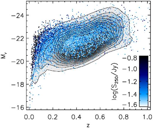
Optical absolute magnitudes in the r band as a function of redshift and 250 μm flux of reliable H-ATLAS IDs (all extragalactic IDs in SDSS), with the background distribution of SDSS shown in contours. The redshifts used are spectroscopic where available, or photometric otherwise. To reduce crowding, we only plot one quarter of the reliable IDs.
5.2 Completeness as a function of redshift and magnitude
We can estimate the completeness of the reliable IDs sample as a function of redshift using a similar statistical analysis to that used to estimate the magnitude distributions in Section 3.1 and in S11. The method is demonstrated in the middle panel of Fig. 11, in which the light grey filled histogram is the redshift distribution of all galaxies from the optical sample that are within 10 arcsec of any SPIRE position: we call this distribution ntotal(z). The darker filled histogram is the distribution of background galaxies that contribute to ntotal(z) but are not directly associated with the SPIRE sources. This distribution, nbkgrd(z), is estimated from the distribution of all redshifts in the full optical catalogue of the three fields, normalized by the ratio of the combined search area around SPIRE positions (π × 10 arcsec 2 × NSPIRE) to the total field area covered by the optical catalogue. The difference ntotal(z) − nbkgrd(z) therefore gives the estimated true redshift distribution of SPIRE counterparts, nreal(z), which is plotted as a dashed orange line, after normalizing by Q0 (the fraction of true counterparts which are within the optical catalogue). The completeness as a function of redshift of the reliable IDs is estimated by the ratio nreliable(z)/nreal(z), where nreliable(z) is the solid black line shown in both the upper and middle panels. The completeness fraction is shown in the lower panel, with error bars based on the assumption of Poisson counting statistics. The completeness of each redshift bin up to z = 3 is shown in Table 6. Compared with the same statistics for SDP (S11), the DR1 completeness is broadly similar, although slightly higher at z > 0.3. This difference may be partly due to cosmic variance, and perhaps due to the greater availability of spectroscopic redshifts in the current work. It is noticeable that the completeness remains relatively high at high redshifts, and in fact appears to be higher at z > 1 than at z ≈ 0.7. This may relate to a dearth of spectroscopic redshifts at 0.5 < z < 1 combined with inaccuracies in photometric redshifts in this range (especially the bias discussed in the previous section). It is also possible that the probability for reliably matching a SPIRE source with its SDSS counterpart (given that it is detected in both surveys) is higher at z > 1 compared to lower redshifts because the magnitude-limited SDSS catalogue is less likely to contain correlated neighbours within the 10 arcsec search radius. Such neighbours would of course reduce the reliability given by equation (16). Equally, the completeness at z < 0.5 is high because the search radius corresponds to a smaller physical scale which is likely to contain fewer neighbours.
Completeness of the reliable sample as a percentage of the total number of true counterparts with r < 22.4, as a function of redshift.
| z | Completeness (per cent) |
|---|---|
| 0.0–0.1 | 91.3 ± 2.2 |
| 0.1–0.2 | 87.7 ± 1.5 |
| 0.2–0.3 | 80.4 ± 1.5 |
| 0.3–0.4 | 72.2 ± 1.3 |
| 0.4–0.5 | 68.9 ± 1.5 |
| 0.5–0.6 | 66.4 ± 1.8 |
| 0.6–0.7 | 60.5 ± 1.7 |
| 0.7–0.8 | 56.2 ± 1.8 |
| 0.8–0.9 | 58.8 ± 3.9 |
| 0.9–1.0 | 65.9 ± 9.9 |
| 1.0–1.5 | 76.1 ± 9.1 |
| 1.5–2.0 | 78.9 ± 9.9 |
| 2.0–2.5 | 76.0 ± 14.0 |
| 2.5–3.0 | 99.6 ± 31.4 |
A similar analysis of the magnitude histograms of true counterparts and of reliable IDs allows us to plot the ID completeness as a function of r-band magnitude in Fig. 14. We see that the completeness is at least 90 per cent for r < 18, but falls to around 65 per cent at r=19.8 (the limiting magnitude of GAMA), and is below 50 per cent for r ≳ 21 (the results are tabulated in Table 7).
![The method of estimating completeness as a function of r-band magnitude from the distribution of all potential extragalactic matches to SPIRE sources [ntotal(m), light grey filled histogram], the background distribution of unassociated galaxies [nbkgrd(m), dark grey filled histogram] and the distribution of reliable IDs [nreliable(m), black solid line]. The difference ntotal(m) − nbkgrd(m) gives the estimated magnitude distribution of true counterparts [nreal(m), orange dashed line]. The estimated completeness given by nreliable(m)/nreal(m) is shown in the lower panel.](https://oup.silverchair-cdn.com/oup/backfile/Content_public/Journal/mnras/462/2/10.1093_mnras_stw1654/2/m_stw1654fig14.jpeg?Expires=1750182121&Signature=UpmaIfv1jYpOM-kLUCTNz0s6Cxmp8zKqiRG1oIfn2jqu~hSIsdkGPQKr98ImLNzAICc0sE~Ld6gPCdRzm1HxhAmHMwGnDiVYh6YudbGQIGAJj-7XefYVyMpf-lI1OB0lnC445wRB-SUn1ULrsU9bj4nIH7pCgPnledZZtCmvRYpairZx2Q1r42qP3n6cpDn2vbPOgDSRL3UcDkK~d5nr5OxP9dgVS2q8EcIOWpO0TClrNFV42n7aqL11H3jrGVBkNS3urULx0fz-hF1ScUGEGfn8NHmw5z95WJaC1Y25k-aTclZa6PFq3SBHOitNsAIVHCynUI3o5MWzSTzC5zMOJg__&Key-Pair-Id=APKAIE5G5CRDK6RD3PGA)
The method of estimating completeness as a function of r-band magnitude from the distribution of all potential extragalactic matches to SPIRE sources [ntotal(m), light grey filled histogram], the background distribution of unassociated galaxies [nbkgrd(m), dark grey filled histogram] and the distribution of reliable IDs [nreliable(m), black solid line]. The difference ntotal(m) − nbkgrd(m) gives the estimated magnitude distribution of true counterparts [nreal(m), orange dashed line]. The estimated completeness given by nreliable(m)/nreal(m) is shown in the lower panel.
Completeness of the reliable sample as a function of r magnitude, for all SDSS IDs and for extragalactic (xgal) IDs.
| r | All optical IDs (per cent) | xgal IDs (per cent) |
|---|---|---|
| 10.0–14.8 | 65.2 ± 15.6 | 106.3 ± 13.0 |
| 14.8–15.2 | 91.2 ± 15.5 | 101.2 ± 12.4 |
| 15.2–15.6 | 96.6 ± 14.3 | 98.6 ± 10.2 |
| 15.6–16.0 | 103.1 ± 11.9 | 100.0 ± 8.2 |
| 16.0–16.4 | 100.8 ± 8.0 | 101.0 ± 6.4 |
| 16.4–16.8 | 99.3 ± 6.1 | 97.5 ± 4.9 |
| 16.8–17.2 | 94.7 ± 4.4 | 95.8 ± 3.9 |
| 17.2–17.6 | 93.8 ± 3.6 | 94.0 ± 3.2 |
| 17.6–18.0 | 92.4 ± 3.0 | 92.2 ± 2.7 |
| 18.0–18.4 | 88.0 ± 2.7 | 88.3 ± 2.4 |
| 18.4–18.8 | 83.7 ± 2.4 | 82.9 ± 2.2 |
| 18.8–19.2 | 77.1 ± 2.1 | 77.6 ± 1.9 |
| 19.2–19.6 | 73.2 ± 1.8 | 72.5 ± 1.7 |
| 19.6–20.0 | 65.4 ± 1.6 | 65.3 ± 1.5 |
| 20.0–20.4 | 60.4 ± 1.5 | 61.2 ± 1.4 |
| 20.4–20.8 | 54.4 ± 1.3 | 54.3 ± 1.2 |
| 20.8–21.2 | 48.6 ± 1.2 | 48.3 ± 1.2 |
| 21.2–21.6 | 45.7 ± 1.2 | 47.2 ± 1.1 |
| 21.6–22.0 | 42.8 ± 1.2 | 45.4 ± 1.2 |
| 22.0–22.4 | 41.5 ± 1.3 | 45.5 ± 1.4 |
6 MULTI-WAVELENGTH PROPERTIES OF H-ATLAS GALAXIES IN GAMA
In this section, we explore the multi-wavelength properties of the subset of H-ATLAS sources with ‘reliable’ counterparts in GAMA, i.e. those with r < 19.8 which are classified as galaxies by Baldry et al. (2010).
6.1 Magnitude distributions
Fig. 15 shows the magnitude distributions in four bands from the UV, optical, near-IR and mid-IR, for reliable IDs with available photometry in each band. For the r band, we can compare both to SDSS and GAMA, but for the other bands we compare to the GAMA photometric catalogue only (Driver et al. 2016). It is noticeable that the H-ATLAS sample selects GAMA sources in the NUV down to a magnitude of around 20, and in W4 down to about 15, with roughly constant efficiency as a function of magnitude. This indicates that H-ATLAS is not biased against blue (UV-bright) star-forming galaxies or hot (22-μm-bright) luminous IR galaxies (LIRGs; which may have been suspected due to the tendency for submm selection to favour cold dusty galaxies). In the r band, H-ATLAS detects and IDs a small fraction of all SDSS sources at all magnitudes, but a large fraction of the galaxies in GAMA at r < 18. Most of the brighter SDSS objects missing from H-ATLAS are stars, which are relatively few in the ID catalogue.
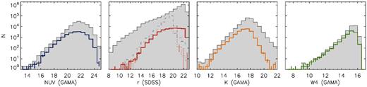
Histograms (solid coloured lines) of the magnitudes of reliable H-ATLAS IDs in NUV, r, K and W4 (22 μm). The background distributions in each band are shown by the filled histogram. The r-band histogram contains all SDSS objects in the optical catalogue (including stars, galaxies and quasars). The dashed grey line shows the distribution of r-band magnitudes in the GAMA galaxy sample. For comparison, we show the magnitude distribution of all reliable IDs in SDSS (solid red line), and that of IDs in GAMA (dotted red line). Photometry in the other bands is drawn from the GAMA photometric catalogue only.
6.2 Optical and IR colours
The stellar population age of a galaxy is roughly traced by its optical colour, since quiescent elliptical galaxies are known to reside in the ‘red sequence’ while active star-forming discs are most likely to appear in the ‘blue cloud’. It has previously been shown (e.g. Dariush et al. 2011) that H-ATLAS selects galaxies in both regions of the colour–magnitude diagram, and in Fig. 16 we show that this is indeed the case in the DR1 sample, both in terms of NUV − r and g − r (rest-frame) colours. The colours have been k-corrected to the rest frame by fitting the FUV − K photometry with kcorrect (Blanton & Roweis 2007). The redder galaxies in H-ATLAS are likely to be reddened by dust attenuation in the optical (Smith et al. 2012), although we also know that a small number of truly passive galaxies are detected in the H-ATLAS sample (Rowlands et al. 2012; Agius et al. 2013). We can infer this by predicting the U − V and V − J colours of the reliable IDs, using kcorrect to reconstruct the colours in the rest-frame SED. The UVJ diagram in Fig. 17 can then be used to define passive galaxies as those falling within the upper-left region (Williams et al. 2009). Fig. 17 shows that a small fraction (8.9 per cent) of sources in the reliable ID sample fall within this region, and these are generally optically luminous. The fraction of the full GAMA sample that falls within the passive region is 35 per cent.
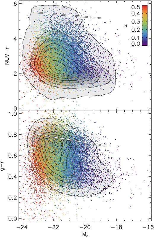
Rest-frame colour–magnitude diagrams in NUV − r and g − r for reliable IDs in GAMA, in comparison to the full GAMA sample (grey-scale contours). The thick dashed line in each panel shows the red sequence derived from the GAMA sample in Bourne et al. (2012). Note that H-ATLAS selects galaxies throughout the full locus of GAMA galaxies.
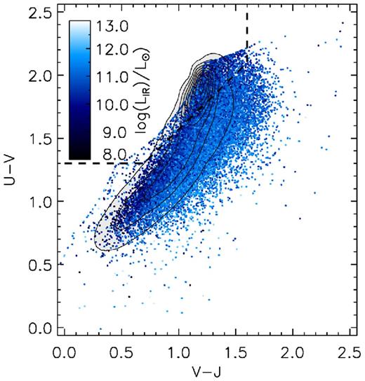
Rest-frame UVJ colour–colour diagrams for reliable IDs in GAMA, in comparison to the full GAMA sample (grey-scale contours). H-ATLAS galaxies are colour-coded by the total IR luminosity estimated from the 100–500 μm photometry as described in Section 6.3. Note that H-ATLAS selects galaxies throughout the full locus of the GAMA sample, including both passive and star-forming galaxies according to the diagnostic given by the dashed line (Williams et al. 2009). The sharp edge seen in the top-left locus of the data is artificial and results from the library of model SEDs within kcorrect, which limit the range of colours in these reconstructed photometric bands.
Mid-IR colours in the WISE bands can be used to classify galaxies according to the emission features resulting from star formation and dust-obscured active galactic nuclei (AGN). In Fig. 18, we show one such classification diagram for galaxies in the reliable ID sample and those in the main GAMA sample that are detected in the W1-W3 bands. The region bounded by the dashed line was defined by Jarrett et al. (2011) to select AGN-dominated mid-IR SEDs, which are generally flat in νLν(λ) while the SEDs of pure star-forming galaxies are rising in the mid-IR. We find that 4.0 per cent of H-ATLAS galaxies are AGN-dominated in the mid-IR, similar to the fraction (6.3 per cent) of GAMA galaxies, although galaxies at higher redshift are clearly more likely to fall within the AGN classification. The WISE colours are not k-corrected, although Cluver et al. (2014) showed that the k-corrected colours in the GAMA sample have a similar distribution to observed colours. Our results are similar to the fraction (5.7 per cent) found in the smaller H-ATLAS SDP sample (Bond et al. 2012) using the same diagnostic.
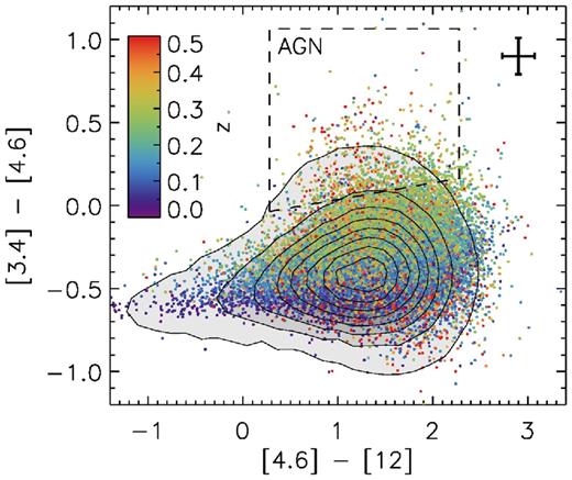
A WISE colour–colour diagram for reliable H-ATLAS IDs in GAMA, compared with the full GAMA sample (grey-scale contours). Only objects detected in all three bands at SNR >3 are plotted. The dashed line delineates the locus of AGN following Jarrett et al. (2011), converted from Vega to AB colours, and the error bars represent the median errors of the H-ATLAS sample.
These fractions relate to the subset of galaxies detected in the three WISE bands plotted. An alternative classification was proposed by Messias et al. (2012) based on the K − [4.5] and [4.5] − [8.0] colours from Spitzer/IRAC photometry, providing a cleaner separation of AGN and star-formation-dominated SEDs at a wide range of redshifts. For the GAMA/H-ATLAS sample, which is predominantly at redshifts z < 0.5, a single colour cut of K − [4.6] > 0.2 should be sufficient to separate SEDs dominated by AGN emission at 4.6 μm (see fig. 3 of Messias et al. 2012). This cut selects 2.7 per cent of H-ATLAS galaxies detected in K and W2, compared with 1.9 per cent of GAMA galaxies. Taking into account upper limits in W2, these fractions become 2.7 ± 0.1 per cent for H-ATLAS IDs, and 0.193 ± 0.003 per cent of GAMA galaxies detected in K (errors represent Poisson counting errors only).
In summary, for the subset of objects detected by WISE, the fraction of mid-IR bright AGN in GAMA and H-ATLAS galaxies is similar, but after removing the WISE detection requirement, there is a slightly raised fraction of AGN in H-ATLAS. This may be interpreted in terms of a link between AGN activity and FIR emission (from star formation or otherwise) but we leave further discussion for dedicated papers.
6.3 Integrated IR luminosities and obscuration of star formation
We estimated total IR luminosities from the PACS and SPIRE fluxes (100–500 μm) by fitting a single modified blackbody with fixed β = 1.82 (Smith et al. 2013), with temperature and normalization as free parameters, and integrating the model in the range 8–1000 μm. This model does not account for the warm dust emitting at λ ≲ 100 μm, and so will underestimate the total luminosity. A better estimate would be obtained by modelling an additional power-law component in the SED at short wavelengths, which can be constrained by including the WISE 22 μm flux (Casey 2012). However, only 14 per cent of our sample are detected at 22 μm, and 9 per cent at 100 μm, so this cannot be constrained for most of the sample. We therefore adopted a single modified blackbody fit to obtain LIR, but applied a correction factor of 1.35 to all galaxies to account for the average contribution from warm dust (e.g. Casey 2012). This approximation will underestimate the total IR luminosity of hotter galaxies, chiefly (ultra)-luminous IR galaxies (ULIRGs, LIR > 1012 L⊙ and LIRGs, LIR > 1011 L⊙), but is sufficient to estimate the luminosities of typical star-forming galaxies on average. Fig. 19 shows the integrated luminosities of the H-ATLAS IDs as a function of redshift. The sample spans a wide range of IR luminosities but becomes dominated by LIRGs at z ≳ 0.25.
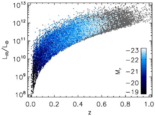
Total IR luminosities of all reliable extragalactic H-ATLAS IDs as a function of redshift. Luminosities were estimated by fitting the 100–500 μm fluxes with a modified blackbody SED with fixed β = 1.82 and free temperature and normalization, and applying a correction factor of 1.35 as described in the text. For the subset of IDs in GAMA, we colour the data by the r-band absolute magnitude measured from kcorrect.
The rest-frame IR-to-UV luminosity ratio was calculated by dividing the integrated IR luminosity (LIR/W) by the rest-frame FUV luminosity (νLν/W). The range of IR/UV ratios probed by H-ATLAS IDs in GAMA/GALEX is similar to that in the Herschel+GALEX-selected sample of Buat et al. (2010). As expected, it is less biased towards high ratios than IRAS-selected LIRGs (e.g. Howell et al. 2010), and less biased towards low ratios than UV-selected samples (e.g. Meurer, Heckman & Calzetti 1999; Kong et al. 2004; Overzier et al. 2011). These other samples have typical log(IR/UV) ∼2 and ∼0–1, respectively, compared with the median log(IR/UV) = 0.95 in the current sample. The IR/UV ratio traces the relative rates of obscured and unobscured star formation, and in Fig. 20 it shows a strong correlation with IR luminosity, and a weaker correlation with the UV spectral index β. We use the GALEX colour βGLX = (log fFUV − log fNUV)/(log λFUV − log λNUV) to estimate β, following Kong et al. (2004). The correlation between IR/UV and β is well documented in the literature, and has been shown to depend strongly on the star formation history, with galaxies dominated by younger stellar populations having higher IR/UV for the same value of β (Kong et al. 2004; Buat et al. 2012). The heterogeneous H-ATLAS sample therefore shows a large amount of scatter in this relationship. At a given value of βGLX, the sample spans a range of IR/UV ratios that encompasses the relationships for starbursts from Kong et al. (2004), and resolved late-type discs from Boissier et al. (2007). The best-fitting relationship from Wijesinghe et al. (2011), based on the H-ATLAS SDP+GAMA sample, unsurprisingly provides a good fit to our sample, but clearly a single IR/UV–β relationship cannot be assumed without accounting for additional variables within the sample.
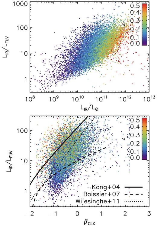
Ratio of rest-frame total IR luminosity to rest-frame FUV-band luminosity (νLν) for H-ATLAS sources which have reliable IDs in GAMA and FUV detections from GALEX, as a function of LIR (top) and βGLX (bottom), where βGLX = (log fFUV − log fNUV)/(log λFUV − log λNUV) as defined by Kong et al. (2004). Also shown in the lower panel are the best-fitting relations for local starbursts (Kong et al. 2004), local late-type galaxies (Boissier et al. 2007) and galaxies selected from the H-ATLAS SDP+GAMA (Wijesinghe et al. 2011).
7 CONCLUSIONS
In this paper, we have described the process of obtaining reliable optical and multi-wavelength counterparts to submm sources in the H-ATLAS DR1 with UV to near-IR data from SDSS, GAMA and other wide-area surveys. The catalogues described in this paper represent a factor of 10 increase in area compared with the previous data release (SDP; S11) and an even greater increase in the number of sources due to improvements in the source extraction described in Paper I.
We searched for counterparts within a radius of 10 arcsec around all ≥ 4σ SPIRE sources in the H-ATLAS catalogues, corresponding to an average flux limit of 27.8 mJy at 250 μm. For the matching catalogue, we used primary objects from SDSS DR7 and DR9 with rmodel < 22.4, removing spurious deblends by visual inspection of objects with deblend flags. We used LRs to measure the reliability of all potential matches in this catalogue, and we also inspected by eye a subset of bright sources to validate the automated process and correct missing ID information for bright galaxies and stars.
The intrinsic fraction of H-ATLAS sources which have a counterpart in the SDSS r < 22.4 catalogue (irrespective of whether the counterpart could be reliably identified) is Q0 = 0.539 ± 0.001 overall (0.519 ± 0.001 for extragalactic objects; 0.020 ± 0.002 for stars). The extragalactic value is significantly lower than that found by S11 in the SDP release, but this can be explained by changes in the methodology leading to an improved estimate of Q0.
While Q0 represents the theoretical maximum identification rate for H-ATLAS sources in SDSS, in reality it is not possible to obtain reliable counterparts for this fraction of sources due to the ambiguity of matching submm sources with a PSF of 18 arcsec to optically detected sources, and the poor correlation between the fluxes in these two wavebands. We found ‘reliable’ counterparts (reliability R ≥ 0.8) for 44 835 submm sources and estimated that this sample has an overall completeness of 73.0 per cent and cleanness of 95.3 ± 0.1 per cent. The sample is dominated by galaxies (97 per cent), although 422 stars and 610 spectroscopically identified quasars are also reliably identified, in addition to 351 quasar candidates (unresolved objects without spectroscopy but with non-stellar colours). The stellar IDs are incomplete and uncertain as a result of poor statistical knowledge of the magnitude distribution of submm-emitting stars; further work in this area would improve the efficiency of the LR procedure for stars. The R ≥ 0.8 reliability cut excludes some sources with multiple optical counterparts (chance alignments, mergers and pairs/groups with small projected separations can all lead to a completely blended submm source), but we estimate that the incompleteness resulting from the existence of multiple counterparts is small (∼1 per cent).
Finally, we investigated some of the multi-wavelength properties of H-ATLAS galaxies with counterparts in GAMA. We measured the redshift distribution of H-ATLAS reliable IDs, which is broadly distributed, peaking between 0.1 < z < 0.8, although there are many H-ATLAS sources that fall below the optical detection limit of SDSS, which are likely to extend to higher redshifts. We showed that there is a poor correlation between submm flux and optical magnitude, but that H-ATLAS is sensitive to a wide variety of galaxy types (classified by colour) similar to that probed by GAMA. For example, H-ATLAS IDs fill the locus occupied by the GAMA colour–magnitude relation in both g − r and NUV − r, and about 9 per cent of H-ATLAS/GAMA matches are classified as passive by their UVJ colours (Williams et al. 2009), compared with 35 per cent of the GAMA sample.
The H-ATLAS galaxies span five orders of magnitude in integrated IR luminosity at z < 0.5, and more than two orders of magnitude in IR/UV luminosity ratio. This sample is far less biased than earlier wide-field FIR-selected samples (e.g. IRAS) and represents a valuable census of dust emission throughout the galaxy population at low to intermediate redshifts, as well as many rare objects at high redshifts.
This H-ATLAS data release provides an important legacy of FIR/submm photometry over a large sky area, and the multi-wavelength catalogue described in this paper has unrivalled potential for studying the interstellar medium and obscured star formation in a large sample of galaxies up to redshift z ≲ 1. All of the data described in this paper and in Paper I are available from www.h-atlas.org.
We would like to thank Michał Michałowski, Hugo Messias and Myrto Symeonidis for advice and enlightening discussions while preparing this paper. NB has received funding from the European Union Seventh Framework Programme (FP7/2007-2013) under grant agreement no. 312725; SD is supported by STFC with an Ernest Rutherford fellowship; and CF acknowledges funding from CAPES (proc. 12203-1). LD, SJM and RJI acknowledge support from European Research Council Advanced Investigator Grant COSMICISM; LD and SJM are also supported by consolidated grant COSMICDUST. SE and EV thank the UK Science and Technology Facilities Council for financial support. MS and SE have received funding from the European Union Seventh Framework Programme ([FP7/2007-2013] [FP7/2007-2011]) under grant agreement no. 607254.
For the least-squares fitting in this work, we have made use of the mpfit package, available from http://purl.com/net/mpfit (Markwardt 2009). The Herschel-ATLAS is a project with Herschel, which is an ESA space observatory with science instruments provided by European-led Principal Investigator consortia and with important participation from NASA. The H-ATLAS website is http://www.h-atlas.org/. GAMA is a joint European-Australasian project based around a spectroscopic campaign using the Anglo-Australian Telescope. The GAMA input catalogue is based on data taken from the Sloan Digital Sky Survey and the UKIRT Infrared Deep Sky Survey. Complementary imaging of the GAMA regions is being obtained by a number of independent survey programmes including GALEX MIS, VST KiDS, VISTA VIKING, WISE, H-ATLAS, GMRT and ASKAP providing UV to radio coverage. GAMA is funded by the STFC (UK), the ARC (Australia), the AAO and the participating institutions. The GAMA website is http://www.gama-survey.org/.
Funding for the SDSS, SDSS-II and SDSS-III has been provided by the Alfred P. Sloan Foundation, the Participating Institutions, the National Science Foundation, the US Department of Energy, the National Aeronautics and Space Administration, the Japanese Monbukagakusho, the Max Planck Society and the Higher Education Funding Council for England. The SDSS website is http://www.sdss.org/. The SDSS is managed by the Astrophysical Research Consortium for the Participating Institutions. The Participating Institutions are the American Museum of Natural History, Astrophysical Institute Potsdam, University of Basel, University of Cambridge, Case Western Reserve University, University of Chicago, Drexel University, Fermilab, the Institute for Advanced Study, the Japan Participation Group, Johns Hopkins University, the Joint Institute for Nuclear Astrophysics, the Kavli Institute for Particle Astrophysics and Cosmology, the Korean Scientist Group, the Chinese Academy of Sciences (LAMOST), Los Alamos National Laboratory, the Max-Planck-Institute for Astronomy (MPIA), the Max-Planck-Institute for Astrophysics (MPA), New Mexico State University, Ohio State University, University of Pittsburgh, University of Portsmouth, Princeton University, the United States Naval Observatory and the University of Washington.
Herschel is an ESA space observatory with science instruments provided by European-led Principal Investigator consortia and with important participation from NASA.
Scottish Universities Physics Alliance.
The NASA/IPAC Extragalactic Database, http://ned.ipac.caltech.edu/, is operated by the Jet Propulsion Laboratory, California Institute of Technology, under contract with the National Aeronautics and Space Administration.
Note that GAMA aperture photometry is only available for r < 19.8 galaxies.
This is the fraction (2572/113 997) of SPIRE 250 μm sources which have reliable optical counterparts with r < 19 and ISOA_r>10 arcsec, although only 710 of them are treated as resolved for photometry purposes in Paper I, while the number of sources that are significantly extended beyond a single beam is much smaller.
Note that such problems are less likely to affect the GAMA photometry which use methods better optimized for galaxies.
Full details of all additions and flags are provided as part of the data release.
Note that the fraction of submm sources with multiple IDs will depend on the flux density regime being considered and on the redshifts of the sources.
REFERENCES
