Spectroscopic identification of type 2 quasars at z < 1 in SDSS-III/BOSS Free

Abstract

1 INTRODUCTION

Much, if not most, of the supermassive black hole growth activity in the Universe is hidden by gas and dust (Antonucci 1993; Lacy et al. 2015). The precise accounting of the demographics of active galactic nuclei (AGNs) of different types and at different redshifts is of significant interest because of the growing realization that the growth of supermassive black holes may have had a strong impact on the evolution of massive galaxies (Tabor & Binney 1993; Silk & Rees 1998; Springel, Di Matteo & Hernquist 2005), especially during the obscured but intrinsically luminous (quasar) phase (Sanders et al. 1988; Hopkins et al. 2006).

Circumnuclear gas and dust make obscured (type 2) AGNs faint at optical, ultraviolet and soft X-ray wavelengths. But luminous type 2 quasars (L_bol ≳ 10⁴⁵ erg s^{− 1}) may be identified using surveys at hard X-ray (Norman et al. 2002; Brandt & Hasinger 2005; Hasinger 2008; Brusa et al. 2010), infrared (Lacy et al. 2004; Martin 2005; Stern et al. 2005; Lacy et al. 2007; Donley et al. 2012; Eisenhardt et al. 2012; Glikman et al. 2012; Stern et al. 2012; Lacy et al. 2013, 2015), and radio (McCarthy 1993; Martínez-Sansigre et al. 2006) wavelengths. However, because different selection methods probe somewhat different populations of objects, there is not yet agreement about the obscuration fraction as a function of redshift and luminosity (Ueda et al. 2003; Brandt & Hasinger 2005; Reyes et al. 2008; Lawrence & Elvis 2010), especially in pencil-beam surveys which contain very few objects at the luminous end of the luminosity function. Very large area surveys are important for discovering such rare sources, and thus despite the suppression of the apparent optical flux by obscuration, ∼1000 type 2 quasars have been selected using their characteristic strong narrow emission lines from the Sloan Digital Sky Survey (SDSS; York et al. 2000), both at low (z < 1, Kauffmann et al. 2003; Zakamska et al. 2003; Hao et al. 2005a; Reyes et al. 2008; Mullaney et al. 2013) and at high (z ≳ 2, Alexandroff et al. 2013; Ross et al. 2015) redshifts.

The Baryon Oscillation Spectroscopic Survey (BOSS; Dawson et al. 2013) is one of the four major surveys of the third phase of SDSS, SDSS-III (2009–2014; Eisenstein et al. 2011). It collected spectra of over a million galaxies (Reid et al. 2016) and over 300 000 quasars (Ross et al. 2012) selected from SDSS imaging data to measure the scale of baryon acoustic oscillations as a function of redshift (Aubourg et al. 2015). The BOSS spectrograph (Smee et al. 2013) covers the range 3600–10400 Å, with a resolution of 1500–2600, depending on wavelength. The BOSS spectroscopic pipeline (Bolton et al. 2012) fits the resulting spectra with templates of common types of objects to provide redshifts and spectroscopic classifications, and measures the strengths and widths of various emission lines. Spectroscopic targeting in BOSS probes fluxes ∼2 mag fainter than those accessible to the SDSS-I/II surveys (Dawson et al. 2013), and thus one might expect that the BOSS survey may be able to uncover a previously missed population of optically obscured type 2 quasars.

This paper selects type 2 quasars from the BOSS spectroscopic data. In Section 2, we describe the sample selection, using various techniques to select z < 0.52 quasars (where standard emission-line ratio selection works well) and those at higher redshift (where the presence of the [Ne v]λ3426 Å line allows us to distinguish AGN from star-forming galaxies). We also identify a significant number of type 2 quasars whose redshifts are incorrectly measured by the BOSS pipeline. In Section 3, we discuss optical and multiwavelength properties of the sample. We summarize in Section 4. We use a h = 0.7, Ω_m = 0.3, Ω_Λ = 0.7 cosmology throughout this paper. While SDSS uses vacuum wavelengths, we quote emission line wavelengths in air following established convention – for example, [O iii]λ5007 Å (hereafter [O iii]) has a vacuum wavelength 5008.3 Å. Objects are identified in the figures by their SDSS spectroscopic ID in the order plate–fibre–Modified Julian Date (MJD).

2 SAMPLE SELECTION

In this paper, we identify type 2 quasar candidates from the complete SDSS-III/BOSS spectroscopic data base (Data Release 12; Alam et al. 2015). The first catalogue of luminous z ≲ 1 type 2 AGNs in the SDSS data (DR1) (Zakamska et al. 2003) was designed to be as inclusive as possible, covering [O iii] luminosities between 3.8 × 10⁴⁰ and 3.8 × 10⁴³ erg s⁻¹, although with completeness and selection efficiency strongly varying with line luminosity (see also Kauffmann et al. 2003; Hao et al. 2005b). In the catalogue by Reyes et al. (2008), we set a minimal luminosity threshold L[O iii] > 3.8 × 10⁴¹ erg s⁻¹, because it was not practical to accurately measure weaker emission lines in moderate-redshift, low-signal-to-noise ratio (SNR) spectra and because we were interested in the objects at the quasar (rather than Seyfert) end of the luminosity range. Zakamska & Greene (2014) carried out a kinematic analysis of the [O iii] emission line of this sample, showing evidence for outflows correlated with radio power and infrared luminosity. This analysis required high-SNR spectra of the emission lines, and thus the sample was further restricted to luminosities L[O iii] > 1.2 × 10⁴² erg s⁻¹.

In this paper, we adopt a somewhat different approach. We rely on the strong empirical relationship between the rest equivalent width (REW) of the [O iii] emission line and its luminosity (Fig. 1) and aim to select type 2 quasar candidates with REW[O iii] > 100 Å as completely as possible. Because [O iii] leaves the BOSS spectral coverage at z ∼ 1, our sample is limited in practice to redshifts below unity. The correlation in Fig. 1 shows that the [O iii] equivalent width cut should result in a sample which is essentially complete at L[O iii] > 3.8 × 10⁴² erg s⁻¹; 92 per cent of the objects in Reyes et al. (2008) with these luminosities have REW[O iii] > 100 Å. Similarly, 56 per cent of the Reyes et al. (2008) objects with L[O iii] between 1.2 × 10⁴²  and 3.8 × 10⁴² erg s⁻¹ have REW[O iii] > 100 Å, so we expect to include about half of the type 2 quasars in the BOSS sample within this luminosity range.

Figure 1.

[O iii] REWs and emission line luminosities of type 2 quasars from the sample presented in this paper (blue) and Reyes et al. (2008, red). While the sample selection is performed using line measurements from the BOSS pipeline, we remeasure [O iii] luminosities and REWs as described in Section 3.2, and these are the values shown in this figure. The vertical dashed line shows our selection criterion REW[O iii] > 100 Å as measured with our fits as described in Section 3.2. There is a strong positive correlation between the equivalent widths and luminosities of the [O iii] emission line.

Open in new tabDownload slide

The optical continuum of type 2 quasars is a poor measure of their intrinsic power since it is suppressed by extinction, but [O iii] emission is thought to arise outside of the obscuring region, and its luminosity is correlated with bolometric luminosity (Heckman et al. 2004). Empirically, in type 1 quasars L_[OIII] = 1.2 × 10⁴² erg s⁻¹ corresponds to an intrinsic (unobscured) absolute AB magnitude of M₂₅₀₀ = −24.0 mag, and 3.8 × 10⁴² erg s⁻¹ corresponds to M₂₅₀₀ = −25.3 mag (Reyes et al. 2008). Therefore, we estimate that the REW[O iii] > 100 Å criterion selects objects that are more luminous than the traditional (though arbitrary) boundary between Seyferts and quasars (M_B ∼ −23 mag), at the bright end of the quasar luminosity function at z < 1 (Richards et al. 2006a; Hopkins, Richards & Hernquist 2007).

In this paper, we define type 1 and type 2 quasars by their classical optical signatures. Specifically, in type 1 quasars, we expect to see both the broad-line region and the narrow-line region, whereas in type 2 quasars the broad-line region is obscured (Antonucci 1993). Therefore, the width of the Balmer lines (Hao et al. 2005a) and the ratio of the strengths of the [O iii] and Hβ lines (Zakamska et al. 2003) play a role in distinguishing type 1 from type 2 quasars. Furthermore, type 2 quasars need to be separated from star-forming galaxies, which also have strong emission lines but with line ratios characterized by underlying ionizing radiation produced solely by stars. We start with objects identifiable using traditional emission line ratio diagnostic diagrams (Baldwin, Phillips & Terlevich 1981; Veilleux & Osterbrock 1987) in Section 2.1. At redshifts z > 0.52, the Hα + [N ii]λλ6548,6583 ÅÅ emission line complex moves out of the BOSS spectral coverage, and we develop an alternative method that utilizes the [Ne v]λ 3426 Å emission line to identify type 2 quasar candidates in Section 2.2. Recovery of type 2 quasars which have been assigned erroneous redshifts by the BOSS pipeline is described in Section 2.3. We present the final sample in Section 2.4.

2.1 Selection at z < 0.52

The majority of extragalactic sources with emission-line optical spectra fall into three categories: (i) star-forming galaxies; (ii) type 1 (broad-line, unobscured) AGNs; and (iii) type 2 (narrow-line, obscured) AGNs. We identify 9454 emission-line objects in BOSS DR12 with REW[O iii] > 100 Å and pipeline redshift z < 1, both as measured by the BOSS pipeline (Bolton et al. 2012). For the initial selection, we use spZline data products¹ for line flux measurements, but we remeasure the [O iii] fluxes and equivalent widths more accurately as a final step of our catalogue presentation in Section 3.2. In this section, we consider only objects flagged as having confident redshift measurements by the BOSS pipeline (i.e. the ZWARNING flag is set to zero; see Bolton et al. 2012), but we return to this issue in Section 2.3. Most of the type 1 AGNs are removed from this sample by the REW cut, as the typical REW[O iii] in these objects is ∼13 Å (Vanden Berk et al. 2001).

Figure 2.

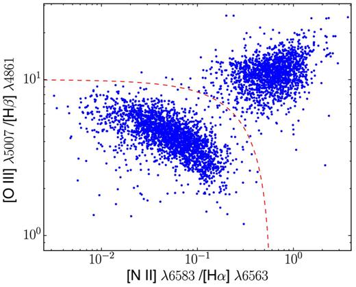
Emission-line ratio diagnostic diagram for 4102 objects with z < 0.52 and REW>100 Å. All measurements are from the BOSS pipeline. Most type 1 AGNs are rejected by this equivalent width criterion, so the majority of sources in the diagram are type 2 AGNs and low-metallicity, low-redshift star-forming galaxies. The dashed line shows our type 2 AGN selection criterion (equation 1).

Open in new tabDownload slide

2.2 Selection at z > 0.52

Various methods have been suggested for separating the spectra of type 2 AGNs from star-forming galaxies at redshifts where the full set of diagnostic emission lines is not available (Zakamska et al. 2003; Reyes et al. 2008; Gilli et al. 2010). In our case, we need to develop new selection criteria to identify type 2 quasar candidates at z > 0.52, when [N ii]λ6583 Å moves out of the BOSS wavelength range.

We use the [Ne v]λ3426 Å emission line to distinguish AGN from star-forming galaxies (Zakamska et al. 2003; Gilli et al. 2010). The ionization energy of Ne⁴⁺ is 97 eV, so the presence of this line implies that the gas has been ionized with intense radiation in the hard UV and soft X-ray range. Star formation produces essentially no emission at these wavelengths, so the mere detection of the [Ne v] emission is an unambiguous sign of the presence of an AGN.

The BOSS pipeline does not automatically measure [Ne v] fluxes, so we measure them using single-Gaussian fits in all candidate spectra. To test how well such [Ne v]-based selection performs, we measure [Ne v] fluxes in AGN and star-forming galaxies with 0.40 < z < 0.52 from the sample shown in Fig. 2. The classification of these objects is already known from the standard diagnostic diagrams. The distribution of the SNR of the [Ne v] line is shown in Fig. 3: only 9 per cent of the objects classified as star-forming by the line ratio criterion of equation (1) have [Ne v] detections; the vast majority of the objects classified as star-forming with [Ne v] detections turn out to be type 1 objects, with broad bases to the Hα lines. The few exceptions all lie close to the boundary between the star-forming and AGN branches in the emission line ratio diagram (Fig. 2), and thus are likely an admixture of the two components.

Figure 3.

[Ne v] SNR distribution of type 2 quasars at 0.4 < z < 0.52 (red histogram), type 2 quasar candidates at z > 0.52 (blue histogram) and a subset of the star-forming galaxies at z < 0.52 (green histogram). The dashed line marks the SNR > 3 cut-off that we choose for our quasar selection for objects with z > 0.52. While approximately 98 per cent of confirmed type 2 quasars at 0.4 < z < 0.52 show [Ne v] SNR > 3, over 91 per cent of star-forming galaxies show no [Ne v] detection with SNR>3.

Open in new tabDownload slide

On the other hand, 98 per cent of the BPT-selected AGNs show significant [Ne v] emission. Thus, the mere detection of the [Ne v] line is indeed a good indicator of the presence of an AGN and results in a fairly complete sample.

There are 4143 objects in BOSS DR12 with z > 0.52 and REW[O iii] > 100 Å. For a source to be selected as a type 2 quasar candidate, we require that the [Ne v] line be detected at SNR>3 in the BOSS spectra for z > 0.52 objects with REW[O iii] > 100 Å. 2191 objects satisfy these criteria. The SNR criterion is of course dependent on the SNR of the BOSS spectra themselves, and we find that the median spectral SNR per pixel of the high equivalent width objects drops steadily from 4 at z = 0.4 to 2.5 at z > 0.6. Thus, our [Ne v]-based selection likely becomes less complete at high redshifts.

The sample at this stage still includes a substantial number of type 1 AGN. Fig. 4 shows the full width at half-maximum (FWHM) of the Hβ line against the ratio of [O iii] to Hβ for the 2191 objects. The sample is clearly bimodal in Hβ line width, which is used as a classical distinguishing characteristic between type 1 and type 2 AGNs at low luminosities (Khachikian & Weedman 1974; Hao et al. 2005a). We choose FWHM(Hβ) = 1000 km s⁻¹ as the cut-off to remove broad-line type 1 AGNs. With this cut, we select 1250 type 2 candidates with z > 0.52, REW[O iii] > 100 Å, [Ne v] SNR > 3 and FWHM(Hβ) < 1000 km s⁻¹. A visual inspection yields 796 type 2 quasars. Most of the candidates rejected by this visual inspection showed weak broad Hβ, broad [Mg ii]λ2800 Å or a strong blue continuum (the latter often associated with narrow-line Seyfert 1 galaxies; see Williams, Pogge & Mathur 2002).

Figure 4.

The relationship between FWHM(Hβ) and [O iii]/Hβ for 2191 AGNs with z > 0.52, REW[O iii] > 100 Å and >3 σ detection of the [Ne v] line. All measurements are from the BOSS pipeline. The objects in the bottom right quadrant have narrow Hβ lines and high [O iii]/Hβ ratios and are likely type 2 AGNs. The objects in the top left have broad Hβ lines and low [O iii]/Hβ ratios (presumably dominated by the broad Hβ component) and are mostly type 1 AGNs. We choose FWHM(Hβ) = 1000 km s⁻¹ (dashed line) as our selection cut to remove broad-line type 1 AGNs. Visual inspection found only 10 objects with broader Hβ lines which belong in the type 2 category.

Open in new tabDownload slide

In the presence of strong quasar-driven outflows, the kinematics of the forbidden-line region can sometimes result in FWHM of the extended emission line region in excess of 1000 km s⁻¹. Indeed, blueshifted asymmetries of the [O iii] line have been recognized as the signature of outflows since the 1980s (Heckman et al. 1981; De Robertis & Osterbrock 1984; Whittle 1985; Wilson & Heckman 1985), although the relationship between outflows and FWHM significantly larger than the depth of the galaxy potential well became clear only much more recently (Nesvadba et al. 2006, 2008; Greene et al. 2009, 2011; Villar-Martín et al. 2011; Hainline et al. 2013; Zakamska & Greene 2014; Zakamska et al. 2016b). To avoid missing the sources with the highest FWHM, we visually inspect the 941 objects in Fig. 4 above the FWHM(Hβ) = 1000 km s⁻¹ cut-off line. We identify an additional 10 type 2 quasars. This is only a small fraction of the strongly kinematically disturbed type 2 quasars in our sample, most of which are identified in the BOSS catalogue using another method (Section 2.3). Our final sample from [Ne v]-based selection at z > 0.52 includes 806 type 2 quasars with z > 0.52.

It is possible that we have been overly aggressive in rejecting objects with weak broad components in Hβ or [Mg ii]λ2800 Å. The problem of weeding out type 1 AGNs with weak broad lines from genuine type 2 candidates is inherently difficult. Even when the direct lines of sight to the nucleus are obscured, some quasar emission can escape along other directions, scatter off the interstellar medium of the host galaxy and reach the observer (Antonucci & Miller 1985; Antonucci 1993; Zakamska et al. 2005). If the scattering is more efficient than a few per cent, then this component can make a noticeable enough contribution to the integrated spectrum of the object that we would see weak broad components in the Balmer and [Mg ii] lines as well as a continuum rising to the blue. Short of conducting polarimetry or spectropolarimetry, we cannot distinguish such objects from type 1 AGN with weak lines and weak continuum. Thus, our selection procedure in which we reject all objects with detectable broad components unfortunately biases our sample against type 2 quasars with high scattering efficiency.

Another problem is that some genuine type 2 quasars show narrow features near [Mg ii]. In Zakamska et al. (2005), He ii λ 2734 Å and C ii λ2838 Å (vacuum wavelengths) are tentatively identified as possible satellite features to [Mg ii]. In lower SNR data or in an object with high velocities in forbidden lines, these features could be blended together and be erroneously interpreted as a broad Mg component. We keep objects without other indications of being type 1 quasars, if the satellite lines are clearly spectroscopically resolved from [Mg ii].

Finally, in unobscured AGNs the region near Mg has strong emission from multiple lines of [Fe II]. In particular, narrow-line Seyfert 1 galaxies show a broad Fe complex peaking at 2300–2400 Å and two Fe complexes on either side of [Mg ii] (Constantin & Shields 2003). Thus, Mg can appear as a narrow core with broad ‘shoulders’ which are actually Fe complexes. Even if such objects show no other signatures of being unobscured, we reject them from our sample. Because we require a high REW of [O iii], a narrow Hβ and low [Fe II] during the visual inspection stage we expect little to no contamination of our sample by narrow-line Seyfert 1 galaxies.

2.3 Selection of type 2s with incorrect/unreliable redshifts

Even though 99.8 per cent of the redshifts that the BOSS pipeline flags as reliable are correct (Adelman-McCarthy et al. 2008; Bolton et al. 2012), there are still some objects with incorrect redshifts in the data base. Type 2 quasars can be among those misclassified objects because there is no proper template for them in the BOSS pipeline. To identify such objects, we explore three ways in which the pipeline is known to respond erroneously to a type 2 spectrum. First, the strong [O iii] emission line of type 2 quasars could be misidentified as Lyα, resulting in a mistakenly high redshift. For example, misidentification of [O iii]λ5007 Å at redshift z_true = 0.5 as Lyα would yield z_wrong = 5.18. Secondly, the [O iii] emission line could be misidentified as Hα, which would result in a mistakenly low redshift. For example, misidentification of [O iii]λ5007 Å at z_true = 0.5 as Hα would yield z_wrong = 0.114. Finally, the redshift could be measured correctly, but the pipeline could indicate that it has low confidence in the result.

In the first possibility, an [O iii] line at z = 0 (i.e. at 5007 Å) misinterpreted as Lyα will be assigned a redshift 3.12. We matched the list of 26 489 BOSS objects with z > 3.12 (as measured by the BOSS pipeline) against the visually inspected (type 1) BOSS quasar catalogue (Pâris et al. 2015); objects that match are presumed to have correct redshifts. Visually inspecting the 1715 objects which remain yields 61 type 2 quasar candidates, whereas the rest are mostly genuine high-redshift type 1 AGNs. All 61 type 2 candidates show strong [O iii] emission. An example of a type 2 quasar selected using this method is shown in the top panel of Fig. 5.

Figure 5.

Example type 2 quasars identified assuming that the BOSS pipeline mistook [O iii] for another strong emission line: for Lyα in the top panel (true redshift z_true = 0.548) and for Hα in the bottom panel (true redshift z_true = 0.5803). Each quasar is indicated with its plate, fibre and MJD (see Section 2.4). These spectra have been smoothed with a 5-pixel boxcar.

Open in new tabDownload slide

In the second possibility, [O iii] is misidentified as Hα, which is only possible for z_true > 0.31. The conversion from observed to rest-frame equivalent width implies that our desired cut of REW[O iii] = 100 Å corresponds to a listed REW for the line, interpreted wrongly as Hα, of 131 Å. An object with Hα with such a high equivalent width is likely to also exhibit strong [O iii]. We thus looked for objects with listed Hα REWs greater than 131 Å, but with REW[O iii] less than 5 Å. This yields 625 objects, of which 369 (well over half) are in fact type 2 quasars at the wrong redshift. Most of the remaining candidates are artefacts with noisy spectra. An example of a type 2 quasar from this selection method is shown in the bottom panel of Fig. 5.

For all selection methods presented so far, we require that the BOSS pipeline be confident about the redshift: the ZWARNING flag (Bolton et al. 2012) must be set to 0. We select another interesting subsample of 1050 type 2s, identifying those objects that the BOSS pipeline flags as having problematic redshift measurements, i.e. non-sky fibres with ZWARNING!=0 with measured REW[O iii] > 100 Å. We visually inspect this subsample and identify 78 type 2s. The BOSS pipeline redshift of these type 2s is essentially always right, despite the ZWARNING flag (indeed, had the redshifts been wrong, the REW[O iii] measurement would have been meaningless).

The 508 type 2 quasar candidates selected in this section are particularly interesting because they tend to show strongly disturbed kinematics in their [O iii] emission lines, which is presumably why their redshifts are either misidentified by the pipeline or the pipeline is not confident about the redshift. This also explains why we see such a clean separation of FWHM(Hβ) in Section 2.2 and Fig. 4: the majority of strongly kinematically disturbed objects with broad forbidden lines are placed at a wrong redshift and are therefore not correctly identified using the [Ne v] SNR cut employed in that section.

2.4 BOSS catalogue of type 2 quasars

We now have 1606 spectroscopic observations of type 2 quasars from Section 2.1, 806 from Section 2.2 and 508 from Section 2.3, adding up to a total of 2920 unique spectroscopic observations. Accounting for objects with multiple spectroscopic observations, our sample represents 2758 unique sources. We provide the full catalogue as an online FITS table. The complete data structure of the catalogue is described in Table 1.

Our basic identification method is by the BOSS Plate and Fibre Number on which this object was observed spectroscopically, together with the MJD of the spectroscopic observation. We also provide right ascension and declination, as measured by the SDSS (Aihara et al. 2011; Ahn et al. 2012). In the cases when the same object has multiple spectra in the data base, we flag the first appearance of the source with a ‘unique’ flag and any subsequent appearances are flagged with the spectroscopic identification of the first available spectrum. The catalogue includes [Ne v] emission line measurements described in Section 2.2, [O iii] emission line measurements described in Section 3.2 and infrared luminosity measurements described in Section 3.3.

3 PROPERTIES OF THE BOSS TYPE 2 QUASARS

3.1 Optical colours and target selection

We present the redshift distribution of each of our subsamples in Fig. 6. The majority (∼85 per cent) of the objects in the final sample lie within the redshift range 0.4 < z < 0.7. This is a reflection of how these objects were selected for spectroscopy in the BOSS survey; 2480 of the type 2 quasars in the final catalogue were targeted as CMASS galaxies. These are selected with a series of magnitude and colour cuts, as described by Reid et al. (2016), to be a roughly stellar mass-limited sample of galaxies (CMASS stands for ‘Constant Mass’).

Figure 6.

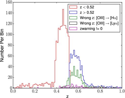
The redshift distribution of our type 2 quasars in Δz = 0.01 bins, showing the five selection criteria. The red histogram corresponds to the 1606 type 2 quasars from Section 2.1; the blue histogram is the 806 type 2 quasars from Section 2.2, and the green, black and magenta histograms correspond to the two samples of wrong-redshift-selected type 2 quasars and the ZWARNING selected sample in Section 2.3. All redshifts are as measured by the pipeline described in Section 3.2.

Open in new tabDownload slide

Fig. 7 shows the SDSS-measured colours (measured using model magnitudes corrected for Galactic extinction following Schlegel, Finkbeiner & Davis 1998) of the objects in the sample as a function of redshift, following Richards et al. (2003). Also shown are median colours for CMASS galaxies in general, as well as for type 1 quasars from SDSS-I/II (Schneider et al. 2010). The type 2 quasars in our sample tend to be appreciably bluer than the bulk of CMASS galaxies in g − r and i − z, but relatively red in r − i. Some of this interesting behaviour is due to the high equivalent widths of the emission lines in type 2 quasar spectra. Specifically, the [O iii] line falls in the i band from redshift 0.4 to 0.6, making the r − i colours relatively red, close to those of CMASS galaxies, and i − z colours blue, close to or even bluer than those of type 1 quasars.

Figure 7.

The observed SDSS colours of objects in our sample as a function of redshift. The red points correspond to those objects with the highest [O iii] equivalent widths. The blue points give the median colours of galaxies selected by the CMASS algorithm (Reid et al. 2016), while the green points are the median for quasars from SDSS-I/II (Schneider et al. 2010).

Open in new tabDownload slide

The continuum colour of our sample is bluer than that of CMASS galaxies, as seen in g − r colours which are not dominated by emission lines, though they are not as blue as those of type 1 quasars. The dominant contribution to the rest-frame ultraviolet continuum of type 2 quasars is likely to be scattered light (Zakamska et al. 2005, 2006; Obied et al. 2016), though star formation is also possible (Wylezalek et al. 2016; Zakamska et al. 2016a). Type 2 quasar hosts are known (Liu et al. 2009) to be even more strongly star-forming than type 1 quasar host galaxies which appear with young stellar populations at these redshifts (Kirhakos et al. 1999; Matsuoka et al. 2014, 2015).

The fact that ∼85 per cent of our type 2 quasars are selected by the BOSS galaxy target selection algorithms means that most of our type 2 quasars are resolved in SDSS imaging. This result is consistent with Reyes et al. (2008); ∼50 per cent of their type 2 quasar sample were selected by the main galaxy target selection algorithm (Strauss et al. 2002). It also suggests that there may be an additional population of unresolved type 2 quasars yet to be identified which reside in compact galaxies; such objects would not be selected by the CMASS targeting algorithm and therefore would not have BOSS spectra.

3.2 Refitting the [O iii] profile

Our sample relies strongly on [O iii] measurements and is limited in REW[O iii]. We initially use the measurements of this quantity from the BOSS pipeline outputs, but these are not ideal: the pipeline fits a single Gaussian to the line, and forces the width of that Gaussian to be the same for all forbidden lines fit. Following Zakamska & Greene (2014), we refit the [O iii] doublet over the rest wavelength range 4910–5058 Å for all our objects, assuming a 2.996:1 intensity ratio for the two [O iii] lines, and forcing the redshifts and profiles of [O iii]λ4959 Å and [O iii]λ5007 Å to be the same. Unlike the extreme objects discussed in Zakamska et al. (2016b), in no case is the [O iii] line broad enough to be affected by the Hβ line, and we thus do not include it in the modelling. The SNR of the spectra in these strong lines is adequate to allow detailed fits. Fits are carried out assuming a linear continuum, and one, two, three or four Gaussians; if adding an extra Gaussian component leads to a decrease in reduced χ² of <10 per cent, we accept the fit with a smaller number of components. The vast majority of the fits require two or three Gaussians; there are only two sources that require four.

These fits give accurate measurements of [O iii] luminosities and equivalent widths; we used these results in Fig. 1. Because these fits are sensitive to wings in the profile that are not fit by a single Gaussian, they tend to give equivalent widths which are systematically higher than those measured by the BOSS pipeline. Specifically, the median REW[O iii] for our type 2 sample as measured by the pipeline is 165 Å, whereas our refits give a median REW[O iii] of 186.0 Å. This means that our sample is somewhat incomplete close to the REW[O iii] limit of 100 Å; there is presumably a population of objects with pipeline equivalent widths somewhat below 100 Å, which would move above this limit with the detailed fits we have described here.

We provide the complete multi-Gaussian decomposition for all sources in the catalogue, as well as the 568 objects with L > 1.2 × 10⁴² erg s⁻¹ in the Reyes et al. (2008) catalogue (Zakamska & Greene 2014), as online FITS tables. The names of the columns in the kinematic catalogue are listed in Table 2. In addition to tabulating the Gaussian components, we provide non-parametric measures of the [O iii] profiles, including the full widths at 25 per cent and 50 per cent of the maximum (in km s⁻¹) and the non-parametric measures defined by Zakamska & Greene (2014) following Whittle (1985). Specifically, for every emission-line profile we measure the velocities v_x at which x per cent of line power accumulates. This allows us to define the widths encompassing 50 per cent, 80 per cent and 90 per cent of line power: w₅₀ ≡ v₇₅ − v₂₅, w₈₀ ≡ v₉₀ − v₁₀ and w₉₀ ≡ v₉₅ − v₀₅, measured in km s⁻¹. These widths are more sensitive to weak broad components than the traditional full width at half-maximum measures. We also tabulate the dimensionless relative asymmetry R ≡ ((v₉₅ − v₅₀) − (v₅₀ − v₀₅))/w₉₀, which is negative for profiles with a heavier blueshifted wing, and dimensionless kurtosis r₉₀₅₀ ≡ w₉₀/w₅₀ which is larger for profiles with heavy wings and narrow cores.

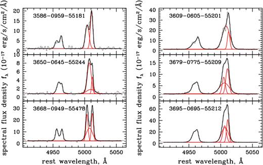
A comprehensive study of the relationships between these measures and their relevance to quasar winds is presented by Zakamska & Greene (2014). In what follows, we use w₈₀ as a measure of the [O iii] kinematics. Fig. 8 shows the profiles and fits for those objects with the objects with the most dramatic outflows, as measured by w₈₀.

Figure 8.

[O iii] spectra of the 10 objects with the broadest [O iii] emission, as measured by the width containing 80 per cent of the line power w₈₀. The spectrum of the [O iii]λ4959,5007 Å region is shown in grey, and the model components (continuum and two or three Gaussians) are shown in red for the 5007 Å line (the fit is performed simultaneously on both lines in the doublet assuming the same kinematic structure). The summed model for both lines of the [O iii] doublet is shown in black. Vertical dashed lines show v₁₀, v₅₀ and v₉₀, so that w₈₀ is encompassed between the left and right lines. The 10 objects shown in the figure have w₈₀ values in the range 2558–3912 km s⁻¹. These values are comparable to the maximal widths found in the Reyes et al. (2008) sample (Zakamska & Greene 2014), but fall short of the extreme values (up to 5409 km s⁻¹) found in high-luminosity red quasars at high redshifts (Zakamska et al. 2016b). Each spectrum is labelled with its plate, fibre and MJD.

Open in new tabDownload slide

In both catalogues, we flag candidate double-peaked [O iii] profiles (see Liu et al. 2010a). While most of these profiles likely result from biconical quasar-driven winds, where each ploughed shell may appear as a separate Gaussian component (Greene, Zakamska & Smith 2012; Harrison et al. 2015), a small fraction of these objects could be due to kpc-scale binary active nuclei (Liu et al. 2010b; Shen et al. 2011; Comerford et al. 2012). Separating these two possibilities is not yet possible without extensive follow-up observations, so we identify possible double-peaked emitters in the catalogue exclusively based on the shape of the [O iii] line. While there is no formal definition of what constitutes a double-peaked profile, for identifying candidate kpc-scale binaries we are interested in profiles with two distinct narrow components in the [O iii] profile which are kinematically separated from one another by an amount comparable to their velocity dispersion.

We identify candidate double-peaked profiles in two ways. First, following Liu et al. (2010a) we identify sources with a minimum in the fitted [O iii] profile and examine them visually. Most of these objects are retained as double-peaked candidates. Secondly, we visually examine all profiles and flag those that do not have a minimum but none the less appear to have two distinct kinematic components. Candidates are visually flagged based on the observed profiles, regardless of whether the two distinct components are accurately captured by the multi-Gaussian fits. Examples of objects from both selection methods are shown in Fig. 9. In the new BOSS sample, 420 of the 2920 spectra show a profile minimum. Of these, 363 (86 per cent) are retained as double-peaked after visual inspection, and an additional 183 without a model profile minimum are identified visually. In the Zakamska & Greene (2014) sample, there are, respectively, 60 and 48 double-peaked candidates identified by the two algorithms.

Figure 9.

Six of the double-peaked candidates in the catalogue. The three objects in the left-hand panels are selected by requiring that the fitted profile has a minimum, whereas the three objects in the right-hand panels are selected by visual inspection. Each spectrum is labelled by its plate, fibre and MJD.

Open in new tabDownload slide

3.3 Crossmatch with AllWISE

The dust within the obscuring medium along the line of sight to a type 2 AGN absorbs much of the energy of optical and ultraviolet photons. This dust emits at mid-infrared wavelengths, to which the dust is more transparent (though obscuration may be significant even at these wavelengths; Nenkova et al. 2008). Thus, observations of type 2 quasars in the mid-infrared may provide a more direct probe of their bolometric emission than the narrow emission lines we have used so far. We matched our sample against the AllWISE (Wright et al. 2010; Cutri et al. 2013) catalogue of the Wide-field Infrared Survey Explorer (WISE) using a 5 arcsec matching radius, picking the nearest match when multiple matches are found. Approximately 97 per cent of the objects in our type 2 quasar sample have a successful match in AllWISE. To estimate the contamination rate, we offset the positions of our sources by 1 arcmin and re-match, resulting in a matching rate of 9 per cent within 5 arcsec. Therefore, a few per cent of our AllWISE matches may be random associations, or have their fluxes contaminated by unrelated objects.

We fit piece-wise power laws between each pair of adjacent WISE bands to determine a flux density, and thus a luminosity (νL_ν) at rest frame 5 and 12 μm. Fig. 10 shows the distribution of our sources in WISE colour space, using the filters at 3.4, 4.6, and 12 μm. The median SNRs of the detections of our objects in the 3.4, 4.6, 12 and 22 μm bands are 26.7, 16.9, 6.8 and 4.0 respectively. The figure also includes type 2 quasars from Reyes et al. (2008); the two distributions are quite similar. The ‘wedge’ denoted by the dashed lines is the luminous AGN selection region as defined by Mateos et al. (2012, 2013), analogous to other proposed mid-infrared colour cuts used for obscured AGN selection (Lacy et al. 2004; Stern et al. 2005, 2012). It is striking that only 34 per cent of our sample is encompassed by this wedge; thus, there is a substantial number of sources with strong optical signatures of a type 2 quasar which would not be identified by the standard colour-based infrared selection criteria.

Figure 10.

The distribution of our sample and that of Reyes et al. (2008) in the WISE ([3.4] − [4.6] versus [4.6] − [12]) colours. The ‘wedge’ denoted by the dashed lines is the luminous AGN selection region as defined by Mateos et al. (2012, 2013). Only 34 per cent of the BOSS type 2 quasars are within this region, indicating that many type 2 quasars would be missed in infrared-selected samples.

Open in new tabDownload slide

In Vega magnitudes, [3.4] − [4.6] ≃ 0 corresponds to the colour of an old stellar population dominated by the Rayleigh–Jeans tail of the spectral energy distribution of stellar photospheres, thus there are few objects bluer than this cut-off. In the absence of any thermal re-emission by dust, this would also be the typical colour of a type 2 quasar whose mid-infrared emission is dominated by the host galaxy. Contribution of warm dust emission moves sources to the right (towards the redder [3.4] − [12] colour) and contribution of hot dust emission moves sources upward (towards the redder [3.4] − [4.6] colour). Type 2 quasars can be obscured even at mid-infrared wavelengths, which is known both from theoretical models (Pier & Krolik 1992) and observations which show that they are significantly redder in the infrared than type 1 quasars (Liu et al. 2013). Therefore, the hot dust contribution is not strong enough in more than half of the sample to push the objects into the mid-infrared wedge. It has been suggested that the objects that lie outside the wedge have WISE fluxes dominated by starlight (Alonso-Herrero et al. 2006; Eckart et al. 2010; Donley et al. 2012; Mateos et al. 2013), but that would be surprising given the high-inferred AGN luminosities for our sample.

3.4 [O iii] properties and bolometric luminosity

Figure 11.

The relationship between [O iii] and rest-frame 12 μm luminosity for the quasars in our sample and those of Reyes et al. (2008). All objects with WISE counterparts are shown here, not just those lying within the wedge of Fig. 10. The solid line is the best-fitting power-law obtained by minimizing perpendicular residuals and the dashed line is the best-fitting linear dependence, with best fits quantified by equations (3).

Open in new tabDownload slide

These should be considered approximate scaling relations, because both our new sample and the Reyes et al. (2008) sample are affected by their respective [O iii] luminosity cut-offs (visible in Fig. 11). Furthermore, there are fewer objects at high luminosity, so that our fit is more heavily weighted by the less luminous objects. The correlation between [O iii] luminosity and 12 μm luminosity is tighter than the one between [O iii] luminosity and 5 μm luminosity (Zakamska & Greene 2014), presumably because the 5 μm luminosity is more strongly affected by geometric effects and dust extinction.

[O iii] kinematics, in turn, can be a useful proxy for the strength of the quasar-driven outflows on host galaxy scales. In low-luminosity AGNs, the kinematics of the forbidden emission lines are strongly correlated with galaxy rotation and/or bulge velocity dispersion (Wilson & Heckman 1985; Greene & Ho 2005), indicating that the emission-line gas is in dynamical equilibrium with the galaxy. This is not the case in quasars (Zakamska & Greene 2014), where the characteristic velocities probed by [O iii] emission are too high to be contained by the galactic potential. The velocity width asymmetry and kurtosis of [O iii] are all correlated with one another, suggesting that any of these values can serve as a proxy for outflow strength. Zakamska & Greene (2014) found that the strongest correlations are between the velocity width of the [O iii] line (as measured by the w₉₀ parameter, Section 3.2), and radio and infrared emission in the Reyes et al. (2008) sample.

In Fig. 12, we investigate the relationship between w₉₀, the velocity width containing 90 per cent of line power, with the [O iii] luminosity, the rest-frame 12 μm luminosity, and the [O iii] equivalent width for the objects in our new BOSS sample. There is no correlation with equivalent width, and a weak one with [O iii] luminosity. The correlation with infrared luminosity, however, is quite strong, suggesting that indeed the velocity width reflects the outflow velocity and that the outflow activity is driven by the bolometric luminosity of the AGN. Zakamska et al. (2016b) have found objects at the peak epoch of quasar activity at z ∼ 2.5 that lie at the extreme end of this diagram – with extremely high infrared luminosities and extremely broad [O iii]; w₉₀ up to 5000 km s⁻¹.

Figure 12.

The relationships between w₉₀ (the velocity width of [O iii] containing 90 per cent of line power) and [O iii] line luminosity, 12 μm infrared luminosity, and [O iii] REW. In each panel, the red points are median values in bins, with the interquartile range indicated. [O iii] velocity width, which is a proxy for quasar wind activity, is most strongly correlated with quasar infrared luminosity.

Open in new tabDownload slide

3.5 Extreme [Ne v] emitters

Our sample includes objects with very strong [Ne v]λ3426 Å emission, including sources with [Ne v]/Hβ > 1. Among type 2 quasars in the Reyes et al. (2008) sample, the mean and standard deviation of the quantity log ([Ne v]/Hβ) are −0.3 and 0.2, respectively, with only 6 per cent of objects showing [Ne v]/Hβ > 1. In our newly selected BOSS sample, these values are, correspondingly, −0.3 dex, 0.3 dex and 13 per cent. The higher fraction of objects with [Ne v]/Hβ >1 is likely due to our explicit selection requirement that [Ne v] be detected in the z > 0.52 subsample.

One example of such an object from the BOSS sample is shown in Fig. 13. In addition to the very strong [Ne v] ([Ne v]/Hβ ≃ 2 in this source), these objects also show unusual emission features at 5721 and 6087 Å, which we identify as transitions of [Fe vii] (Rose, Elvis & Tadhunter 2015a). The ionization potentials of [Ne v] and [Fe vii] are 97 and 99 eV, respectively, almost identical, and thus it is not surprising that the strength of these features are strongly correlated.

Figure 13.

The BOSS spectrum (smoothed with a 5-pixel boxcar) of an extreme [Ne v] emitter from the newly selected BOSS sample. Prominent emission lines are marked. The [O iii] and Hα line peaks are offscale. The stellar continuum is also apparent, showing Calcium K absorption and a strong Balmer break.

Open in new tabDownload slide

Figure 14.

The SDSS image of Mrk 266. The image is 51.2 arcsec on a side; north is up and east is to the left. This is a gri colour composite, prepared following the approach of Lupton et al. (2004). The squares indicate the regions which have SDSS spectra; the SDSS image deblender identified the blue region in the north as a separate ‘galaxy’. The northernmost spectrum was identified using our spectroscopic search for objects with high equivalent width, high-ionization emission lines. The blue colour of the nebular emission in this region is due to the strong [O iii] dominating the g-band emission in this extended nebula.

Open in new tabDownload slide

Rose et al. (2015a,b) deem such objects ‘coronal line forest AGNs’ and explore the hypothesis that these emission lines arise from the inner wall of the obscuring material. It is thus rather unusual to see these features in type 2 quasars, where it is expected that the line of sight to this emitting region should be obscured. Rose et al. (2015b) argue that even in the classical unification model with a toroidal obscuring region, a small fraction of viewing directions might result in both strong coronal lines and obscured broad-line region (another such example from the Reyes et al. 2008 sample is analysed by Villar-Martín et al. 2011). This picture is consistent with the distribution of dust temperatures in these objects and in type 2 quasars, in that coronal-line AGNs are warmer as inferred from the infrared colours than are other type 2 quasars. The statistics of the coronal-line AGNs in the type 2 population might offer clues to the geometric structure of the obscuring material and provide constraints on its clumpiness (Nenkova, Ivezić & Elitzur 2002).

3.6 Extended emission-line region

One intriguing object identified using our initial selection is the spectrum of an extended emission-line region associated with the merging pair Mrk 266 (Fig. 14), photoionized by the AGN in one of the merging nuclei. This region of ionized gas, roughly 12 kpc from the central nucleus (Hutchings, Neff & van Gorkom 1988; Ishigaki et al. 2000; Mazzarella et al. 2012), has essentially no associated starlight, and thus displays [O iii] with a very high equivalent width. Another well-known example of such an extended emission line nebula with AGN line ratios is Hanny's Voorwerp (Lintott et al. 2009), which is found near a galaxy which no longer hosts an active nucleus but presumably did in the recent past. A systematic search for such objects in the SDSS data is conducted by Sun et al. (in preparation). We removed the off-nuclear spectrum of Mrk 266 from the sample because it is not an integrated spectrum of the entire galaxy.

3.7 Composite spectrum

We construct a composite spectrum from our sample by shifting all spectra to their rest frames (using the adopted redshifts listed in the catalogue), rebinning the spectra on to a common rest wavelength grid and calculating the error-weighted average. In Fig. 15, we further normalize the composite spectrum by a continuum obtained by spline-interpolating between relatively line-free regions. In this presentation, the overall continuum shape is lost, but the equivalent widths of the features are preserved. We provide the composite spectrum in an online FITS table. The high-SNR continuum reveals a multitude of emission features due to the quasar-ionized gas and absorption features due to the stellar photospheres and interstellar medium of the host galaxies.

Figure 15.

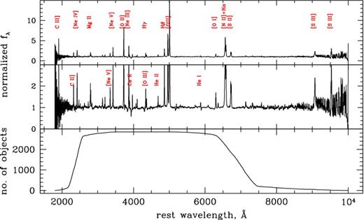
The composite spectrum of all BOSS type 2 quasars normalized by an approximate continuum obtained by spline-interpolating between relatively line-free regions. The top spectrum shows the brightest emission lines, the middle panel shows a zoom in on the same data, and the bottom panel shows the number of objects contributing at each wavelength. Only a small subset of all detected lines are marked, following line identifications by Vanden Berk et al. (2001).

Open in new tabDownload slide

4 CONCLUSIONS

In this paper, we present a sample of 2758 type 2 (obscured) quasars at z ≲ 1 selected from the SDSS-III/BOSS spectroscopic data base. We aim to select sources with high equivalent width emission lines, REW([O iii]λ5007 Å) > 100 Å. At low redshifts (z < 0.52), we use standard emission-line diagnostic diagrams to separate type 2 candidates from star-forming galaxies. At higher redshifts (z > 0.52), when Hα and other diagnostics move out of the BOSS spectral coverage, we require a detection of [Ne v]λ3426 Å which requires ionization by an AGN and narrow Hβ to separate type 2 quasars from type 1 quasars.

An interesting subsample of 508 objects has erroneous or uncertain redshifts in the SDSS data base. We select such sources by assuming that [O iii] – one of the strongest lines in the type 2 quasar spectra – is mistaken for another strong line, either Lyα or Hα, by the pipeline. Additionally, we examine sources with high REW of [O iii] and with redshifts flagged by the SDSS data base pipeline as uncertain. These sources tend to have strongly kinematically disturbed emission lines and they are therefore poorly matched against the standard templates. Because our selection algorithms for such sources are not exhaustive, small numbers of interesting type 2 quasars with broad [O iii] could remain unidentified in the SDSS spectroscopic data base.

While in low-luminosity AGNs, the kinematics of the forbidden emission lines tend to trace the potential of the AGN host galaxy, in powerful quasars [O iii] profile shapes appear to be strongly related to quasar-driven winds. We conduct multi-Gaussian decomposition of [O iii] for all objects in this sample and calculate all commonly used non-parametric measures of [O iii] profile shape. We release complete kinematic decomposition information for both the new catalogue of BOSS type 2 quasars and for our previous kinematic analysis of 568 luminous (L[O iii] > 1.2 × 10⁴² erg s⁻¹) type 2 quasars selected from SDSS I/II (Reyes et al. 2008; Zakamska & Greene 2014). We also identify 654 candidate objects with double-peaked [O iii] profiles which could be interesting for studies of quasar-driven winds or of binary AGNs.

As we determine by matching the sample to the WISE survey, the type 2 quasars presented here have high infrared luminosities, with median νL_ν = 1.7 × 10⁴⁴ erg s⁻¹ at rest frame 5 μm and 4.2 × 10⁴⁴ erg s⁻¹ at rest frame 12 μm. If quasars were isotropic emitters at 12 μm, we could apply a typical bolometric correction at this wavelength of ∼9 (Richards et al. 2006b) to estimate the median bolometric luminosity of our sample to be ∼4 × 10⁴⁵ erg s⁻¹. Intriguingly, despite very high luminosities, fewer than half of the objects in our sample have [3.6 − 4.5] colour red enough for them to be selected using the common infrared colour selection methods used to identify AGNs. Thus, it is likely that type 2 quasars are obscured even at mid-infrared wavelengths, so that hot dust emission from the inner parts of the obscuring material remains largely invisible to the observer (Liu et al. 2013). Therefore, the bolometric corrections are likely higher than those for type 1 quasars, and so then is our estimated median bolometric luminosity.

The demographics of quasars remain an interesting unsolved problem in astronomy, with obscured quasars now thought to play an important role in galaxy evolution. This work, alongside other approaches, makes it clear that different selection methods result in largely different samples of objects. Samples selected by infrared, optical and X-ray methods overlap at the tens of per cent level (Lacy et al. 2013), but none of the selection methods results in a complete sample. The combination of multiwavelength approaches and extensive studies of samples selected at different wavelengths will be required to measure the demographics of quasars and to determine the geometry and the spatial structure of the obscuring material.

Funding for SDSS-III has been provided by the Alfred P. Sloan Foundation, the Participating Institutions, the National Science Foundation and the US Department of Energy Office of Science. The SDSS-III website is http://www.sdss3.org/.

SDSS-III is managed by the Astrophysical Research Consortium for the Participating Institutions of the SDSS-III Collaboration including the University of Arizona, the Brazilian Participation Group, Brookhaven National Laboratory, Carnegie Mellon University, University of Florida, the French Participation Group, the German Participation Group, Harvard University, the Instituto de Astrofisica de Canarias, the Michigan State/Notre Dame/JINA Participation Group, Johns Hopkins University, Lawrence Berkeley National Laboratory, Max Planck Institute for Astrophysics, Max Planck Institute for Extraterrestrial Physics, New Mexico State University, New York University, Ohio State University, Pennsylvania State University, University of Portsmouth, Princeton University, the Spanish Participation Group, University of Tokyo, University of Utah, Vanderbilt University, University of Virginia, University of Washington, and Yale University.

REFERENCES

SUPPORTING INFORMATION

Additional Supporting Information may be found in the online version of this article:

Reyes_kinematics.fits

Type2s.fits

Type2s_composite.fits

Type2s_kinematics.fits

(Supplementary Data).

Please note: Oxford University Press is not responsible for the content or functionality of any supporting materials supplied by the authors. Any queries (other than missing material) should be directed to the corresponding author for the article.