


Abstract
In diffuse molecular clouds, possible precursors of star-forming clouds, the effect of the magnetic field is unclear. In this work, we compare the orientations of filamentary structures in the Polaris Flare, as seen through dust emission by Herschel, to the plane-of-the-sky magnetic field orientation (Bpos) as revealed by stellar optical polarimetry with RoboPol. Dust structures in this translucent cloud show a strong preference for alignment with Bpos. Of the field orientations, 70 per cent are consistent with those of the filaments (within 30°). We explore the spatial variation of the relative orientations and find it to be uncorrelated with the dust emission intensity and correlated to the dispersion of polarization angles. Concentrating on the area around the highest column density filament, and on the region with the most uniform field, we infer the Bpos strength to be 24–120 μG. Assuming that the magnetic field can be decomposed into a turbulent and an ordered component, we find a turbulent-to-ordered ratio of 0.2–0.8, implying that the magnetic field is dynamically important, at least in these two areas. We discuss implications for three-dimensional field properties, as well as for the distance estimate of the cloud.
1 INTRODUCTION
The structure of interstellar clouds is highly complex, characterized by the existence of elongations, or filaments, of various scales (e.g. Myers 2009). The Gould Belt Survey conducted by the Herschel space observatory captured the morphologies of the nearby molecular clouds with unprecedented sensitivity and detail, allowing the study of filamentary structures to advance (e.g. André et al. 2010). A better understanding of filament properties and their relation to their environments could provide clues as to how clouds proceed to form stars.
To this end, important questions to answer are whether the magnetic field interacts with filaments and how this interaction takes place. Its role in the various stages and environments of star formation is hotly debated. In simulations of super-Alfvénic turbulence, magnetic fields are tangled due to the gas flow (e.g. Ostriker, Stone & Gammie 2001; Falceta-Gonçalves, Lazarian & Kowal 2008). In such models, filaments are formed by shock interactions (Heitsch et al. 2001; Padoan et al. 2001) and the magnetic field within them is found to lie along their spines (Heitsch et al. 2001; Ostriker et al. 2001; Falceta-Gonçalves et al. 2008). In studies of sub/trans-Alfvénic turbulence, where the magnetic field is dynamically important, filament orientations with respect to the large-scale ordered field depend on whether gravity is important. In simulations where gravity is not taken into account (e.g. Falceta-Gonçalves et al. 2008) or structures are gravitationally unbound (Soler et al. 2013), filaments are parallel to the magnetic field. However, self-gravitating elongated structures are perpendicular to the magnetic field (Mouschovias 1976; Nakamura & Li 2008; Soler et al. 2013). Both configurations are the result of the magnetic force facilitating flows along field lines. Finally, if the magnetic field surrounding a filament has a helical configuration (Fiege & Pudritz 2002), then the relative orientation of the two as projected on to the plane of the sky can have any value, depending on projection, curvature and whether the field is mostly poloidal or toroidal (Matthews, Wilson & Fiege 2001).
The relation between cloud structure and the magnetic field was highlighted early on by observational studies (e.g. in the Pleiades; Hall 1955). On cloud scales, Li et al. (2013) found that the distribution of relative orientations of elongated clouds and the magnetic field (both projected on to the plane of the sky) is bimodal: clouds either tend to be parallel or perpendicular (in projection) to the magnetic field. In a series of papers, the Planck collaboration compared the magnetic field to the interstellar medium (ISM) structure across a range of hydrogen column densities (NH). Planck Collaboration XXXII (2016a) considered the orientation of structures in the diffuse ISM in the range of NH ∼ 1020–1022 and found significant alignment with the plane-of-the-sky magnetic field (Bpos). Planck Collaboration XXXV (2016b) found that, in their sample of 10 nearby clouds, substructure at high column density tends to be perpendicular to the magnetic field, whereas at low column density there is a tendency for alignment.
Studies of optical and near-infrared (NIR) polarization, tracing Bpos in cloud envelopes, show that dense filaments within star-forming molecular clouds tend to be perpendicular to the magnetic field (Pereyra & Magalhães 2004; Alves, Franco & Girart 2008; Chapman et al. 2011; Sugitani et al. 2011). However, there are diffuse linear structures, called striations, that share a common smoothly varying orientation and are situated either in the outskirts of clouds (Goldsmith et al. 2008; Alves de Oliveira et al. 2014) or near dense filaments (Palmeirim et al. 2013). These structures show alignment with Bpos (van den Bergh 1956; Chapman et al. 2011; Palmeirim et al. 2013; Alves de Oliveira et al. 2014; Malinen et al. 2016). The extremely well-sampled data of Franco & Alves (2015) in Lupus I show that Bpos is perpendicular to the cloud's main axis but parallel to neighbouring diffuse gas. There are, however, exceptions to this trend (e.g. L1506 in Taurus; Goodman et al. 1990).
While the large-scale magnetic field has been mapped in many dense molecular clouds, little is known about the field in translucent molecular clouds. In this paper, we investigate the relation of the magnetic field to the gas in the Polaris Flare, a high-latitude diffuse cloud. This molecular cloud extends above the galactic plane and is at an estimated distance between 140 and 240 pc, although this is debated (e.g. Zagury, Boulanger & Banchet 1999; Schlafly et al. 2014). It is a translucent region (AV ≲ 1 mag; Cambrésy et al. 2001) devoid of star formation activity (André et al. 2010; Men'shchikov et al. 2010; Ward-Thompson et al. 2010), except for the existence of possibly pre-stellar core(s) in the densest part of the cloud MCLD 123.5+24.9 (MCLD123; Ward-Thompson et al. 2010; Wagle et al. 2015). Signatures of intense velocity shear have been identified in this region and have been linked to the dissipation of supersonic (but trans-Alfvénic) turbulence (Hily-Blant & Falgarone 2009, and references therein).
The dust emission in ∼16 deg2 of the Polaris Flare has been mapped by Herschel (Pilbratt et al. 2010) as part of the Herschel Gould Belt Survey (André et al. 2010; Miville-Deschênes et al. 2010; Men'shchikov et al. 2010; Ward-Thompson et al. 2010). The Planck space observatory has provided the first map of the plane-of-the-sky magnetic field in the area at a resolution of tens of arcmin (Planck Collaboration XIX 2015a; Planck Collaboration XX 2015b). In Panopoulou et al. (2015, hereafter Paper I), we presented a map of the plane-of-the-sky magnetic field in the same area, measured by stellar optical polarimetry with RoboPol. The resolution of optical polarimetry (pencil beams) and coverage of our data allow for a detailed comparison between the magnetic field and cloud structure. The goal of this work is to compare the magnetic field orientation to that of the linear structures in the Polaris Flare and to estimate the plane-of-the-sky component of the field in various regions of the cloud. In Section 2.1, we present the distribution of relative orientations of filaments and Bpos throughout the mapped region. We compare properties such as the relative orientations and polarization angle dispersion across the map in Section 2.2 and we present the distribution of filament widths in Section 2.3. We analyse two regions of interest separately in Section 2.4 and estimate the Bpos strength in these regions in Section 2.5. Finally, we discuss implications of our findings in Section 3 and summarize our results in Section 4.
2 RESULTS
2.1 Relative orientations of |$\boldsymbol {B_{\rm pos}}$| and dust filaments
We use the Herschel-SPIRE 250-μm map1 in our analysis of cloud structure. Filamentary structures are evident throughout the Herschel image of this translucent cloud. We compare the orientations of these structures to the optical polarization data presented2 in Paper I, shown as line segments on the 250-μm dust emission image in Fig. 1. The segment length is proportional to the (debiased) fractional linear polarization, pd. A line showing a pd of 2 per cent is located in the bottom-left corner and a line of 1 pc length is located in the top left. We adopt a distance of 150 pc to be consistent with the analysis of Herschel data in the literature (based on Heithausen 1999). The rectangles highlight regions of interest that are referred to in the following analysis. The panels on the right show enlarged versions of both regions. A preliminary inspection of the map shows that the orientation of Bpos revealed from optical polarimetry seems to correlate well with the apparent orientations of filaments in most of the map. This correlation can be quantified by measuring the relative orientation of the two.
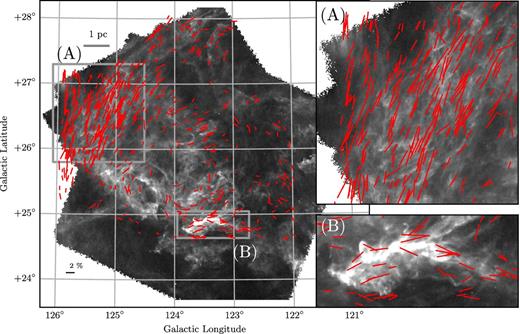
Herschel 250-μm image of the Polaris Flare (grey-scale). Segments are the optical polarization data from Paper I. Regions A (striations) and B (MCLD123), indicated by the rectangles in the full map, are shown in the top-right and bottom-right panels for detail. Scales of 1 pc and pd = 2 per cent are shown in the top-left and bottom-left corners of the full map.
An excellent tool for determining the orientation of linear structures, irrespective of their brightness, is the rolling Hough transform (RHT; Clark, Peek & Putman 2014). It was introduced in the study of diffuse H i and has also been used in analyses of molecular clouds (Koch & Rosolowsky 2015; Malinen et al. 2016). The RHT quantifies the linearity of cloud structure for every image pixel. It does so by measuring the intensity along any given direction within a disc region surrounding each pixel. The RHT returns the probability that a pixel is part of a linear structure as a function of angle. Integrating for all angles results in a visualization of linear features in the image (RHT backprojection).
We have applied the RHT to the Herschel 250-μm image and we present the RHT backprojection in Fig. 2. The darkest pixels in the image belong to well-defined linear structures in intensity (filaments and striations). Apart from these structures, the RHT backprojection contains some spurious features (e.g. in the bottom part of the map where dust emission is very faint or absent). These features seem correlated with the Herschel scanning direction. Because neither cloud structure nor magnetic field orientation coincide with this direction, the effect of these features on the distribution of relative orientations will be to randomize a very small number (if any) of values, introducing misalignment.

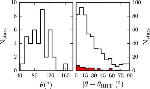
The polarization segments tracing the orientation of Bpos are overplotted on the backprojection in Fig. 2. At the position of each polarization measurement, we calculate the mean RHT angle (θRHT, defined as in Clark et al. 2014), within a circle of diameter 0.17 pc (corresponding to an angular diameter of 4 arcmin). We then compare θRHT to the orientation of each polarization segment, θ, by taking the absolute value of their difference,3 |θ − θRHT|. There are 39 polarization measurements that extend outside the dust emission image and are not included in the comparison to cloud structures. The distribution of the relative orientations for the 570 remaining measurements is plotted in Fig. 3. There is a strong preference in alignment: 70 per cent of polarization measurements are within 30° of the orientation of linear features in their surrounding gas. A Monte Carlo run showed that the probability of obtaining this correlation by chance is less than 10−6. Only 8 per cent are within 30° of being perpendicular to their surrounding gas. We explored the effect of changing the parameters of the RHT, as well as the area around each star used in calculating θRHT, and found no significant variation for a large portion of the parameter space.
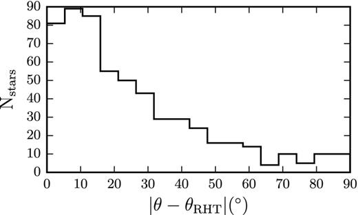
Distribution of the absolute difference between the angle of each polarization segment and the RHT angle in its vicinity (|θ − θRHT|). The distribution contains all 570 polarization measurements that lie in the Herschel image.
2.2 Variation across the field
The results presented above on the alignment of filaments and Bpos concerned the entire map. However, both field and cloud structure are not homogeneous across the cloud. For example, there is a low column density area of striations, marked by the rectangle as region A in Fig. 1, where Bpos exhibits ordered structure. Adjacent to this area, towards lower latitude and longitude, in a significant portion of the map, measurements are sparse and polarization angles show substantial dispersion.
The various trends existing in the measured cloud properties can be better visualized by constructing maps of average (smoothed) quantities across the sky. The maps are constructed by creating a grid (5-arcmin squares) of the field. The value at each grid centre is calculated by averaging the values of star measurements within 10 arcmin of it. The final map is smoothed using a boxcar filter of 5 arcmin width. Fig. 4 shows such maps of various quantities: (a) number of significant stellar polarization measurements (pd/σp ≥ 2.5); (b) Herschel 250-μm intensity; (c) polarization angle, θ; (d) scatter of θ; (e) |θ − θRHT|; (f) pd. Only bins with at least five measurements were used to produce the maps (reducing this number to three did not make a qualitative difference).
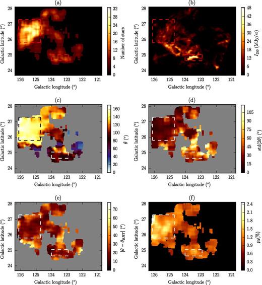
Quantities smoothed on a 5 × 5 arcmin2 grid: (a) number of stellar polarization measurements; (b) Herschel 250-μm intensity; (c) polarization angle; (d) polarization angle scatter; (e) relative orientation of Bpos and filaments; (f) fractional linear polarization. Rectangles outline regions A and B.
The number of significant stellar polarization measurements is highest in region A, which is the bright part in the upper left of the map in panel (a). The number density (per 5-arcmin bin) in this area is more than twice that in the rest of the map. Smaller local maxima are found: (i) in region B; (ii) in the centre of the map (123| $_{.}^{\circ}$|5, +26| $_{.}^{\circ}$|3); (iii) above the striations at (124| $_{.}^{\circ}$|5, +27| $_{.}^{\circ}$|5). As noted in Paper I, this variation in the number of measurements is not due to variations in stellar density across the field, or due to systematics such as observing conditions. Panel (b) shows the Herschel 250-μm image smoothed with a boxcar filter of 5-arcmin width. The MCLD123 filament (region B) stands out as a maximum of intensity. By comparing the number density of significant stellar polarization measurements to the dust emission intensity (panels a and b), we find that the overall structure of the two maps is significantly different. Therefore, the variation of the density of significant polarization measurements cannot be attributed to variations in the column density.
The relative orientation of Bpos and the filamentary structures in the cloud, shown in panel (e), are very similar to the std(2θ) map. Regions characterized by a large polarization angle dispersion appear to coincide with regions where filaments are perpendicular to Bpos. The preference in alignment throughout the map, seen in Fig. 3, is evident, as regions with |θ − θRHT| ≲ 20° (dark) occupy most of the map area.
The highest values of pd (panel f) are in the region of the striations. The Planck polarized intensity peak coincides with the brightest part of this map at (126°, +27°) (see figure A.1 in Planck Collaboration XX 2015b). The second, but lower, local maximum in pd is in region B. The spatial variation of pd resembles that of Nstars. This correlation is evident in Fig. 5 (top left), where the average value of Nstars is plotted for each (equally populated with pixels) pd bin. This correlation is natural, as the polarization measurements were selected in Paper I to satisfy pd/σp ≥ 2.5. Because the observational errors σp are uniform across the field (Paper I), it is more likely that a larger number of significant measurements will be obtained in regions of higher pd.
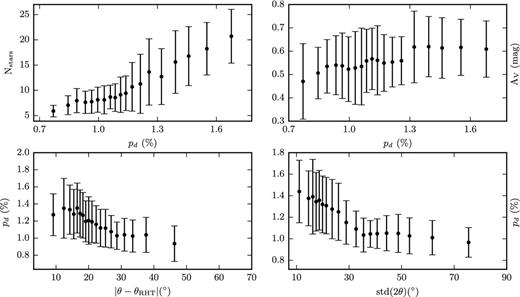
Binned pixel-to-pixel comparison of maps from Fig. 4: top left, Nstars versus pd; top right, extinction AV versus pd; bottom left, pd versus |θ − θRHT|; bottom right, pd versus std(θ). Error bars show the ±1σ from the mean in each bin. Bins contain the same number of pixels.
Additional support for the fact that the variation in the number of significant polarization measurements is uncorrelated with the column density is given by the plot in the top-right panel of Fig. 5, where the visual extinction AV (from the map of Cambrésy et al. 2001) is plotted against pd (from panel f of Fig. 4). One possibility that explains the observed variation of Nstars is that the three-dimensional (3D) orientation of the magnetic field varies significantly throughout the sky. If this were true, then we would expect more significant polarization to be detected in regions where the field is mostly on the plane of the sky. In these regions, pd should be higher and this is consistent with the correlation of pd and Nstars that we find. Also, if the field strength is more significant than turbulent gas motions, which tend to randomize its orientation (see Section 2.5), regions where Bpos is stronger (high pd, Nstars) should have a small angle scatter. This is indeed the case, as can be seen in the bottom-right panel of Fig. 5. However, a significant contribution to this trend is likely to be coming from the larger measurement error of lower-significance measurements (near the cut of pd/σp ≥ 2.5).
If the assumption of a strong magnetic field holds, then diffuse, non-self-gravitating filaments such as the ones in this cloud are expected to be mostly parallel to the 3D field orientation. So, if the field lies mostly on the plane of the sky, the alignment of the projected field and filaments will be easily detected. However, if the field is mostly along the line of sight, then filaments and field can be observed as having any relative orientation. A hint of such a trend may exist in the bottom-left panel of Fig. 5. Planck Collaboration XXXII (2016a) find this exact trend (their fig. 13) and attribute it to the same effect: the projection of the 3D field on the sky. The anticorrelation of pd with std(θ) is also observed (fig. 21 of Planck Collaboration XIX 2015a).
Planck Collaboration XXXII (2016a) also find that the degree of alignment decreases with column density in the range NH = [1020, 1022] cm−2. In contrast to this, it is evident even visually that panels (b) and (e) in Fig. 4 are uncorrelated – we see no sign of such a trend. It is possible that the range of column densities in the Polaris Flare is significantly different than that in Planck Collaboration XXXII (2016a). To investigate whether this is the case, we convert the range of AV in the Polaris Flare to NH using the standard relation of Bohlin, Savage & Drake (1978): NH = 1.9 × 10²¹AV (cm−2 mag−1). From the AV map of Cambrésy et al. (2001), values in the cloud vary within AV = [0.2, 1.2] mag ⇒ NH = [0.4, 2.3] × 1021 cm−2. Because the Cambrésy et al. (2001) data have a low resolution (8 arcmin), this range might be underestimated. Indeed, the cores in MCLD123 have NH ∼ 1022 cm−2. Therefore, the range of NH in the cloud is comparable to that of Planck Collaboration XXXII (2016a), who infer that the anticorrelation of alignment with column density is most likely due to the existence of molecular cloud structures that are perpendicular to the magnetic field. The only available explanation for this observation is that matter in magnetically dominated self-gravitating clouds collapses preferentially along field lines, producing structures that are elongated and perpendicular to the field. If we accept this reasoning, then it should not come as a surprise that we do not find such a trend in the gravitationally unbound Polaris Flare.
In summary, the above correlations seem to indicate the presence of a strong magnetic field in the cloud, which might change orientation from being mostly parallel to the plane-of-the-sky in region A to being more inclined in other areas.
2.3 Filament widths
An important morphological characteristic of filaments is their width. We use the Filament Trait-Evaluated Reconstruction (filter) method4 (Panopoulou et al. 2014) to construct the width distribution of filaments in the Herschel image. filter takes as input the skeleton of an image and finds the width of the elongated structures. For this purpose, a Gaussian is fit to the radial profile at every point along the filament axis, and the resulting FWHM is deconvolved by the beam size. The skeleton is produced by disperse (Sousbie 2011), which is a topological code that can extract the filamentary structures of an image. It is designed to connect local maxima (cores). This property renders the construction of a representative skeleton difficult, because a significant part of the Polaris Flare does not contain bright cores. As seen in Fig. 2, the RHT produces a visualization of filamentary structures irrespective of brightness. This enables us to apply disperse to the RHT backprojection image and to obtain a representative skeleton of the Herschel image to use as input to filter.
The distribution of filament widths in the Herschel image is shown in Fig. 6. The distribution has a peak at 0.06 pc and a spread of σw = 0.04, twice as much as the typical error in the width determination (σfit) in our implementation of the code. The intrinsic spread of the distribution is |$\sigma _{\rm int} = (\sigma _{\rm w}^2 - \sigma _{\rm fit}^2)^{1/2} = 0.035$| pc. Although lower than the characteristic width of 0.1 pc (e.g. Arzoumanian et al. 2011; Koch & Rosolowsky 2015), the peak value found here falls within the spread of the distributions from these works.
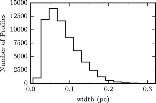
Distribution of widths along filaments in the Herschel image.
We investigate whether there are trends in the distribution of widths across the cloud, by constructing a smoothed map of the widths found by filter (Fig. 7). We use a boxcar filter of the same size as the maps in Fig. 4 (5 arcmin, or 0.2 pc) to allow for a better visual comparison. The map shows fluctuations in the width of filaments that do not appear to have any large-scale systematic trend. This remains the case for maps with smaller smoothing kernels. However, when comparing the distribution of widths within region A (Fig. 8, left, dotted red line) to that of the rest of the map (solid black line), we find that the former is slightly shifted towards lower values. A Kolmogorov–Smirnov (KS) test rejects the hypothesis that the two originate from the same parent distribution at the 0.001 level. In constructing the distributions, we discard structures with lengths less than 0.2 pc, as these have aspect ratios that are too small to be considered filamentary. There is an indication that the shift towards lower widths becomes more pronounced as we raise this threshold to 0.4 pc.
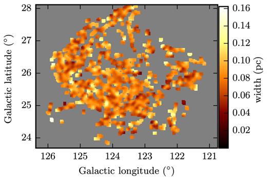
Map of filament widths found with filter, smoothed with a 5-arcmin boxcar filter.
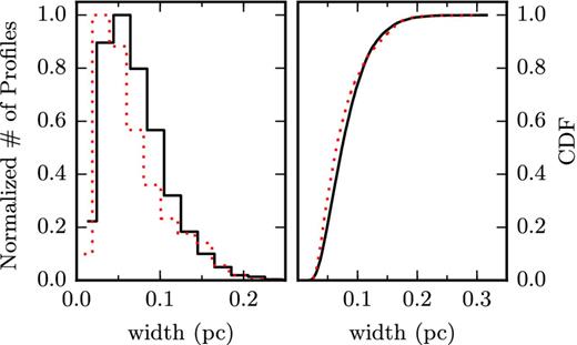
Left: normalized distribution of widths found with filter in the entire map (solid black) and in region A (dotted red) for all structures longer than 0.2 pc. Right: CDF of the same distributions.
2.4 Analysis of regions A (striations) and B (MCLD123)
Having explored the various observed properties of the cloud and their variation across the map, we now focus on the two regions of interest defined in Fig. 1.
2.4.1 Region A (striations)
Region A contains striking features both in dust emission (see the appendix of Miville-Deschênes et al. 2010) and in polarization (Fig. 1). Both Bpos and striation orientations throughout the area are ordered. This is apparent in the distribution of polarization angles shown in panel (a) of Fig. 9. The distribution of θ resembles a normal distribution with a mean at −20° and a standard deviation of δθobs = 11°. The mean observational error (panel b) is 7| $_{.}^{\circ}$|6, while the 80th percentile of the distribution is 10°. Therefore, a significant contribution to the observed spread is due to the measurement error.
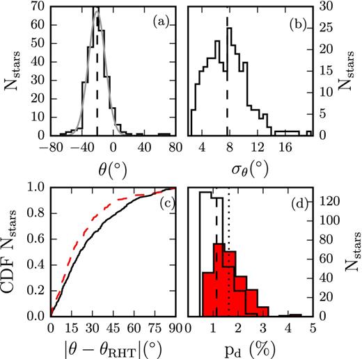
(a) Polarization angle distribution in region A (black solid), Gaussian fit (grey), average (dashed). (b) Distribution of polarization angle measurement errors in region A (solid) and mean (dashed). (c) Normalized CDFs of relative orientations of polarization measurements and dust striations in region A (dashed red) and the rest of the map (solid black). (d) Distributions of pd in region A (filled red) and the rest of the map (empty black); dashed and dotted lines are their average values.
In addition to this uniformity, the mean directions of the field and dust structures appear to be aligned and this occurs to a greater extent than in the rest of the map. This is supported by the comparison of the normalized cumulative distribution functions (CDFs) of |θ − θRHT| shown in Fig. 9, panel (c). Inside the region (dashed red line) 75 per cent of the differences |θ − θRHT| lie in the range [0°, 30°], whereas outside (solid black) only 63 per cent are in the same range.
Another characteristic of region A is that it exhibits a higher fractional linear polarization than the rest of the map, as seen in panel (f) of Fig. 4. We compare the distribution of pd in region A (filled red) and in the rest of the map (black empty) in panel (d) of Fig. 9. It is clear that pd in the region extends to higher values than out of the area, and that the mean pd (dashed line, out; dotted line, in) is lower outside the region.
2.4.2 Region B (MCLD123)
Region B shows a different picture than region A. In this area, which is the densest part of the cloud, the plane-of-the-sky field seems to bend along the MCLD123 filament. The left panel of Fig. 10 shows the distribution of θ for this region while the right panel shows the distribution of relative orientations, |θ − θRHT|, for region B (filled red) and the rest of the map (empty black). The mean of the distribution of θ is 90°, and the standard deviation is 25°. The spread is partly due to the large-scale curvature of Bpos in the vicinity and on the MCLD123 filament. The values of |θ − θRHT| show a slight preference for alignment, although they extend to angles consistent with orthogonality.
Left: distribution of polarization angles in region B. Right: distribution of |θ − θRHT| for region B (filled red) and the rest of the map (empty black).
2.5 Magnetic field strength and comparison to turbulence
The role of the magnetic field in the two regions discussed above can be investigated further by estimating the strength of the plane-of-the-sky magnetic field and by comparing the magnetic energy to that of turbulent motions.
2.5.1 Turbulent-to-ordered field ratio
We implement the method of Hildebrand et al. (2009) and Houde et al. (2009) – hereafter the H09 method – in regions A and B. We calculate the dispersion function 〈Δθ2(l)〉tot, as explained above, we correct it to obtain the left side of equation (6) and we fit the function on the right side of equation (6) to these values with respect to l2. The fit takes into account the error of 〈Δθ2(l)〉tot. In Fig. 11, we plot |$\langle \Delta \theta ^2(l) \rangle _{\rm tot}- \sigma ^2_{\rm M}$| with distance l, for each region (black solid lines). The black dots in Fig. 11 show the values used for the fit. The fits |$p(l) = m^2l^2 + b^2(1-e^{-l^2/2\delta ^2})$| are shown with red dashed lines. The distances are shown on a logarithmic scale (the bins used for fitting were linear). The bin size in region B (1.5 arcmin) was chosen so that there were more than 10 points per bin (in the fitting range). The bin size (1.7 arcmin) for region A was the minimum that produced a positive value of |$\langle \Delta \theta ^2(l) \rangle _{\rm tot} - \sigma ^2_{\rm M}$| for the first bin. A choice of bin size larger by up to 38 per cent in region A, and 33 per cent in region B, produces values of b and δ within the error of the fit. The fits were done considering only distances smaller than the scale at which Bpos varies (l < d). In region A, we performed the fits up to l ≈ 20 arcmin. In region B, we fit the data up to l ≈ 13 arcmin. The choice of d is that which permits the maximum number of bins to be used in the fit while providing a fit that traces the exponential cut-off as well as possible. In region A, both b and δ remain within the error of the fit for a choice of d in the range 8–25 arcmin. The same holds for region B in the range 9–13 arcmin.
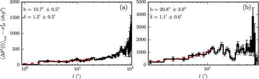
The dispersion function (corrected for measurement errors) versus angular distance, l, for regions A (left) and B (right). The red dashed line shows the best-fitting function of the form |$\langle \Delta \theta ^2(l) \rangle _{\rm tot} -\sigma _{\rm M}^2 = m^2l^2+ b^2(1-e^{-l^2/2\delta ^2})$|. The black dots show the data points that were used in the fits. The fit results for b and δ are shown in the top left.
The results of the fits are shown in the top left of the panels in Fig. 11. The correlation length of Bt is not well constrained, as it is only in the first bin of region A that the effect of the exponential decay in equation (8) is apparent. The values for δ obtained for both regions are consistent within the errors of the fits. Inserting the values for b and δ from the fits into equation (8) we obtain estimates for the ratio |$\langle B^2_{\rm t} \rangle ^{1/2}/B_0$|: 0.2–0.5 for region A and 0.3–0.8 for region B. The line-of-sight depth of each region used for these estimates is presented and discussed in the next section.
2.5.2 Strength of the ordered component
Having inferred the value of δθ from the H09 method, we now move on to find the values of the remaining quantities that enter into equation (3) and we use them to obtain an estimate for Bpos in both regions. Table 1 presents the values used in obtaining these estimates.
Values used for estimation of Bpos in regions A and B: ΔV, FWHM of CO (J = 1–0) line; AV, average visual extinction (Cambrésy et al. 2001); NH, hydrogen column density; slos, line-of-sight dimension; nH, hydrogen number density; δθH09, polarization angle dispersion from the H09 method (equation 4); δθ, polarization angle dispersion from Section 2.4.1 (corrected for measurement error according to equation 11); |$\langle B^2_{\rm t} \rangle ^{1/2}/B_0$|, turbulent-to-ordered field ratio from the H09 method; |$B^{\rm H09}_{\rm pos}$|, plane-of-sky magnetic field using δθH09 and equation (3); |$B^{\rm mDCF}_{\rm pos}$|, plane-of-sky magnetic field using δθ and the modified equation (3) as explained in the text.
| Region | ΔV | AV | NH | slos | nH | δθH09 | δθ | |${\sqrt{\langle B^2_{\rm t}\rangle }}/{B_0}$| | |$B^{\rm H09}_{\rm pos}$| | |$B^{\rm mDCF}_{\rm pos}$| |
|---|---|---|---|---|---|---|---|---|---|---|
| (km s−1) | (mag) | 1020 (cm−2) | (pc) | (cm−3) | (°) | (°) | (μG) | (μG) | ||
| A | 3.1 | 0.6 | 12 | 0.4–1.3 | 300–1000 | 10°–29° | 8 | 0.2–0.5 | 24–120 | 43–81 |
| B | 2.6 | 0.7 | 24 | 0.25–0.5 | 1500–3100 | 17°–44° | 0.3–0.8 | 30–111 |
The gas mass density is equal to ρ = μmHnH, where mH is the mass of the hydrogen atom, μ = 1.36 is a factor that accounts for the fraction of helium and nH is the total hydrogen number density. The total nH must be used and not |$n_{{\rm H}_{2}}$| because even though the cloud is molecular, the fraction of gas that is in atomic form might be important (|$N_{{\rm H}\,\scriptscriptstyle {\rm I}} \sim N_{{\rm H}_{2}}$|; Hily-Blant & Falgarone 2007). To estimate the density in region B, we assume that MCLD123 has a cylindrical geometry. This implies a line-of-sight dimension of ∼0.25–0.5 pc, where the lower bound is twice the observed extent of the dense part of the filament and the upper bound is found to include the more diffuse parts. The average |$N_{{\rm H}_{2}}$| from the map of André et al. (2010) is 8 × 1020 cm−2, corresponding to NH ∼ 2.4 × 1021 cm−2. Dividing by the assumed line-of-sight dimension gives nH ≃ 1500–3100 cm−3 (see also Grossmann et al. 1990).
We can obtain a loose constraint on the mean density of region A by arguing that it is likely to be less than that of region B (as the latter contains cores). An upper bound would therefore be |$n_{\rm H}^{\rm A} < n_{\rm H}^{\rm B}$|. A lower limit on the density can be estimated by considering existing measurements of nH from ultraviolet data of stars in diffuse sightlines. A set of measurements from various works has been collected by Goldsmith (2013) who shows that most sightlines with NH ≳ 1021 cm−2 ⇒ |$N_{\rm H_2} \gtrsim 3 \times 10^{20}$| cm−2 have measured densities: 300 ≳ nH ≳ 60 cm−3 (assuming |$N_{{\rm H}\,\scriptscriptstyle {\rm I}} \simeq N_{\rm H_2}$|). The column density in region A is estimated5 by |$N_{\rm H}^{\rm A} \simeq N_{\rm H}^{\rm B} \, I_{250}^{\rm A}/I_{250}^{\rm B} \simeq 1.2 \times 10^{21}$| cm−2, where we have assumed that the temperature distribution is quasi-uniform throughout the cloud (Men'shchikov et al. 2010; Schneider et al. 2013) so that intensity (I250) variations in the Herschel image are mostly caused by NH fluctuations. Because the Polaris Flare is a molecular cloud, we reason that |$n_{\rm H}^{\rm A} > 300$| cm−3 (the upper limit from the aforementioned sightlines) is an appropriate approximation. The line-of-sight dimension of region A is then (|$s_{\rm los} = n^{\rm A}_{\rm H}/N^{\rm A}_{\rm H}$|) 1.3 ≳ slos ≳ 0.2 pc. The upper limit is approximately one-third of the size of the region as projected on the sky, while the lower limit is similar to the assumed slos in region B. We expect that the true slos lies mostly near the lower limit of this range because, as a result of the translucent nature of the cloud, the line-of-sight dimension should not be very large. Studies of cirrus clouds in general find a high likelihood of them being sheet-like (e.g. Gillmon & Shull 2006). Along with the fact that regions A and B have similar mean AV (Table 1), this implies that slos in the two regions should not vary by orders of magnitude.
To estimate the velocity dispersion δv, we use the 12CO (J = 1–0) data from the survey of Dame, Hartmann & Thaddeus (2001).6 The data, first presented by Heithausen et al. (1993), cover 134 deg2 including the Herschel-mapped area. The angular resolution is 8.7 arcmin and the spectral resolution is 0.65 km s−1. We fit a Gaussian to the mean spectrum of each region and relate its FWHM (ΔV) to the velocity dispersion (δv) with |$\delta v = \Delta V/(2 \sqrt{2\ln 2})$|. Complications can arise when 12CO (J = 1–0) is used to estimate the velocity dispersion if the line is optically thick. However, Hily-Blant & Falgarone (2007) found that the 12CO (J = 1–0) line is optically thin in diffuse gas within the MCLD123 filament with column density derived from the scaling of CO to 13CO velocity-integrated line temperatures: |$N_{\rm H_2} \sim 10^{20}$| cm−2. Because the mean column density in region A is |$N_{\rm H_2} \approx 4 \times 10^{20}$| cm−2 (|$N_{{\rm H}\,\scriptscriptstyle {\rm I}} \approx N_{\rm H_2}$|) this indicates that the line might also be optically thin within region A. The line is most likely optically thick in the densest parts of region B; however, these occupy a very small fraction of the area considered.
The results that follow from equation (3) are presented in Table 1. We show the entire range of values, given the possible variation in the estimated quantities. The range arises from two factors: the error on δ and the estimate of slos, which enters both in the estimation of the density ρ and in the dispersion of polarization angles from the H09 method. The Bpos estimates between regions A and B are very similar.
Hily-Blant & Falgarone (2007) obtained an estimate of B ≃ 15 μG for a smaller part of region B, using the angle dispersion of filaments seen in 12CO. This value is 50 per cent that of the lowest bound of our estimate.
2.5.3 Bpos with alternative estimate of δθ
We can obtain an alternative estimate of Bpos by using the observed angular dispersion δθobs found in Section 2.4.1 from the Gaussian fit to the distribution of polarization angles (see, for example, section 4.2.3 of Barnes et al. 2015). Ostriker et al. (2001) applied the method of Davis (1951) and Chandrasekhar & Fermi (1953) to numerical simulations of MHD turbulence using this type of angle dispersion calculation and found that the method provides a good estimate of Bpos when δθ ≲ 25°. They introduced a factor f in equation (3) to correct for line-of-sight averaging: |${B_{\rm pos}} = f \sqrt{4\pi \rho } \,\delta v/\delta \theta$| and proposed f ≈ 0.5.
The values for the magnetic field strength are shown in the last column of Table 1. They lie within the range of values found using the angle dispersion from H09 and the original equation (3).
3 DISCUSSION
3.1 Properties of the three-dimensional magnetic field
increased alignment efficiency (e.g. more background radiation, a larger amount of asymmetric dust grains, larger grain sizes), that is, higher factors p0 and/or R;
more uniform magnetic field along the line of sight, that is, higher F;
increased Bpos (inclination of B is larger with respect to the line of sight), that is, higher cos γ.
Several pieces of evidence challenge the validity of case (i). First, if the radiation illuminating region A were very different in intensity or direction, then the dust temperature of the area would have to be qualitatively different (higher) than in other regions of the cloud. As mentioned in Section 2.5, the results from Men'shchikov et al. (2010) imply that temperature and density variations are subtle across the field. Indeed, the temperature probability distribution function presented by Schneider et al. (2013) is narrow. Also, the most likely candidate for providing illumination to the cloud, because of its likely proximity, is Polaris (the star). By studying optical and 100-μm light from MCLD123, Zagury et al. (1999) concluded that the star cannot be the primary source of dust heating. Additionally, larger amounts of (aligned) grains would imply larger column densities (or AV) than the rest of the cloud, which is not a characteristic of region A. To the best of our knowledge, there is no evidence for significant variation of grain size within the same cloud between regions of such similar AV.
Finally, if the 3D orientation of the magnetic field is mostly in the plane of the sky in region A and less so in other parts of the cloud, this could also explain the increased measurement density in this region. We can estimate the change in angle that is needed to obtain the difference in pd between regions A and B, from equation (12). Taking all factors equal between the two regions except the inclination angle, the ratio of pd is |$p_{\rm d}^{\rm A}/p_{\rm d}^{\rm B} = 1.63/1.3 = \cos ^2\gamma _{\rm A}/\cos ^2\gamma _{\rm B}$|. This ratio could arise either from a pair of large γA, γB with a small difference or from small angles having a large difference. This ambiguity can be avoided by considering the expected polarization angle dispersions for different inclinations of the magnetic field, studied with MHD simulations by Falceta-Gonçalves et al. (2008). In their work, these authors found that in the range 0°–60° the predicted polarization angle dispersions are below 35° for their model with a strong magnetic field (Alfvén Mach number 0.7). Because the angle dispersions in the two regions are significantly lower than this value, it is safe to assume that 0° < γA, γB < 60°. For this range, we find that the observed ratio of pd can be explained by inclination differences most likely in the range γB − γA = 6°–30°. In order to explain the difference in pd between region A and the lowest mean-pd region in the map (Fig. 4, panel f, approximately at the centre of the map) which has a pd ∼ 0.7 per cent, the difference in inclination angle needs to be 20°–50°.
With the existing set of measurements, we are not able to conclude whether the variations in polarization fraction are mostly due to change in inclination or due to differences in the uniformity of the field along the line of sight. However, we have provided bounds on the areas of the parameter space in which these differences are likely to occur.
3.2 Cloud distance
In the literature, there is no definitive consensus on the cloud's distance. The existing estimates are shown in Table 2 along with the method that was used to obtain each one.
Heithausen & Thaddeus (1990) base their distance estimate on reddening estimates of stars in the field from Keenan & Babcock (1941), who found reddened stars from distances as close as 100 pc and found that all stars farther than 300 pc were reddened. Knowing that Polaris (the star) showed dust-induced polarization, and that the then existing distance estimates to the star were 109–240 pc, they placed the cloud at a distance d < 240 pc. This distance fits with the smooth merging of the cloud at lower latitudes with the Cepheus Flare, at 250 pc.
Zagury et al. (1999) compared IRAS 100-μm emission with optical images of MCLD123 and found that the brightness ratios are consistent with Polaris (the star) being the illuminating source of the cloud in the optical. They placed the cloud at a distance 6–25 pc in front of the star (105 < d < 125 pc from the Sun) so that its contribution in dust heating would be minimal compared to the interstellar radiation field.
Brunt et al. (2003) used principal component analysis (PCA) of spectral imaging data to infer distances based on the universality of the size–linewidth relation for molecular clouds. Their estimate is consistent with both the above estimates.
Schlafly et al. (2014) used accurate photometry measurements of the Panoramic Survey Telescope and Rapid Response System 1 (Pan-STARRS1) and calculated distances to most known molecular clouds. Their estimate for the distance of the Polaris Flare (390 pc), was obtained for lines of sight in the outskirts of the cloud (outside our observed field).
In Fig. 12 (top), we zoom in on the region surrounding the North Star and overplot the polarization data (red) and the measurement of the North Star (white) from the Heiles (2000) catalogue on the Herschel image. The lengths of the segments are proportional to their pd, and the length of the Heiles measurement has been enhanced 10 times. The position of the North Star is marked with a blue star. The star happens to be projected on an area of very little dust emission, hence the low pd. Magnetic field orientations in the area show a strong peak around 110°, with a few measurements (which happen to fall towards the right and bottom of the area) clustering around 40°. This can be seen in the distribution of angles in the area shown in Fig. 12 (bottom). The polarization angle of the North Star (Heiles 2000) is shown with the dark grey vertical line and the light grey band shows the 1σ error. The stars that are nearest to Polaris, in projection, belong to the peak at 100°. The fact that the orientation of the North Star's polarization is consistent with this peak is intriguing. It could add to the evidence supporting that Polaris is behind the Flare, constraining its distance to the Zagury et al. (1999) estimate. However, because the orientation of stellar polarization shifts by a substantial amount (60°) in ∼20 arcmin, denser sampling of the area is needed in order to ascertain this indication.
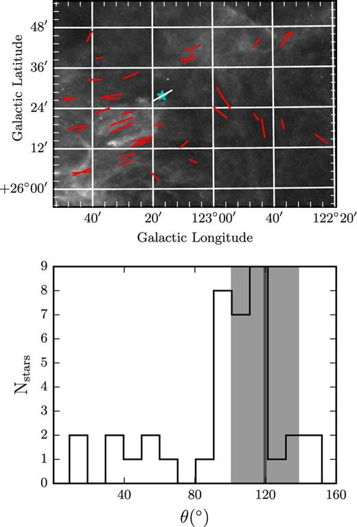
Top: polarization angle of the star Polaris (Heiles 2000), white segment, compared to our data, red segments. The pd of Polaris is 0.1 per cent, but has been enhanced 10 times. Its position is marked with a star. Bottom: distribution of θ in the area shown in the top panel. The dark grey line shows the θ of Polaris while the grey band is the 1σ error. Bin size is 10°.
4 SUMMARY
We have combined RoboPol optical polarization measurements and Herschel dust emission data to infer the magnetic field properties of the Polaris Flare. We have found that linear dust structures (filaments and striations) are preferentially aligned with the projected magnetic field. This alignment is more prominent in regions where the fractional linear polarization is highest (and the number of significant polarization measurements is largest). This correlation supports the idea that variations in the alignment are partly caused by the projection of the 3D magnetic field. We investigated the possibility of important spatial variations in the filament widths and found only a slight indication of such an effect. Using the Davis (1951), Chandrasekhar & Fermi (1953) and Hildebrand et al. (2009) methods, we estimated the strength of the plane-of-the-sky field and the ratio of turbulent-to-ordered field components in two regions of the cloud: one containing diffuse striations, and the other harbouring the highest column density filament. Our results indicate that the magnetic field is dynamically important in both regions. Combining our results, we find that differences of 6°–30° in the magnetic field inclination between two cloud regions can explain the observed polarization fraction differences. This difference can also be explained by a difference in the line-of-sight dispersion of the field of 10°–25°. Finally, we find that the polarization angles of the North Star (Heiles 2000) and of RoboPol data in the surrounding area favour the scenario of the cloud being in front of the star.
The authors thank L. Cambrésy for providing the extinction map and S. Clark and E. Koch for helpful advice on their codes. We also thank D. Blinov, J. Liodakis, R. Skalidis, A. Tritsis and E. Palaiologou for their help throughout the duration of this project. We are grateful to M. Houde for his comments on the manuscript and to P. F. Goldsmith and D. Clemens for useful scientific discussions. Finally, we thank the anonymous reviewer for insightful comments that helped to significantly improve the manuscript. GVP and KT acknowledge support by FP7 through the Marie Curie Career Integration Grant PCIG-GA-2011-293531 ‘SFOnset’ and partial support from the EU FP7 Grant PIRSES-GA-2012-31578 ‘EuroCal’. This research has used data from the Herschel Gould Belt Survey (HGBS) project (http://gouldbelt-herschel.cea.fr). The HGBS is a Herschel Key Programme jointly carried out by SPIRE Specialist Astronomy Group 3 (SAG 3), scientists of several institutes in the PACS Consortium (CEA Saclay, INAF-IFSI Rome and INAF- Arcetri, KU Leuven, MPIA Heidelberg), and scientists of the Herschel Science Center (HSC).
Formerly, Institute for Plasma Physics.
The map is part of the preliminary data available at the Herschel Gould Belt Survey archive.
Following the publication of the catalogue of 609 measurements in Paper I, we discovered an error in the conversion from the polarization angle with respect to the North Celestial Pole to the angle with respect to the North Galactic Pole. This error affected the orientation of 77 segments in the top of the published map. We have corrected the formula used for the conversion and have updated the values of the galactic angle in the published catalogue. This updated version is used in this work and can be found at http://cds.u-strasbg.fr/. No other changes have been made to the original release.
All angles are defined with respect to the North and increase towards the East, according to the International Astronomical Union (IAU) convention.
The code is available at https://bitbucket.org/ginpan/filter.
Survey online archive can be found at https://www.cfa.harvard.edu/rtdc/CO/IndividualSurveys/.
REFERENCES
