


Abstract
We present an analysis of the gas-phase oxygen abundances of a sample of 28 galaxies in the local Universe (z < 0.02) hosting Type Ia supernovae (SNe Ia). The data were obtained with the 4.2 m William Herschel Telescope. We derive local oxygen abundances for the regions where the SNe Ia exploded by calculating oxygen gradients through each galaxy (when possible) or assuming the oxygen abundance of the closest H ii region. The sample selection only considered galaxies for which distances not based on the SN Ia method are available. Then, we use a principal component analysis to study the dependence of the absolute magnitudes on the colour of the SN Ia, the oxygen abundances of the region where they exploded and the stretch of the SN light curve. We demonstrate that our previous result suggesting a metallicity dependence on the SN Ia luminosity for non-reddened SNe Ia can be extended to our whole sample. These results reinforce the need of including a metallicity proxy, such as the oxygen abundance of the host galaxy, to minimize the systematic effect induced by the metallicity dependence of the SN Ia luminosity in future studies of SNe Ia at cosmological distances.
1 INTRODUCTION
Type Ia supernovae (SNe Ia) are claimed to be thermonuclear explosions of carbon–oxygen white dwarfs (CO WDs; Hoyle & Fowler 1960). Their origin is not well established, since there is still an open discussion about the different possible progenitor scenarios. The single-degenerate scenario (Whelan & Iben 1973; Nomoto 1982) occurs when a WD in a binary system accretes mass from its non-degenerate companion until the Chandrasekhar mass limit (∼1.44 M⊙) is reached. At that moment, the degenerate-electron pressure is not longer supported, and the thermonuclear explosion occurs. On the other hand, the double-degenerate scenario (Iben & Tutukov 1984; Webbink 1984) consists of two CO WDs gravitationally bounded that lose angular momentum and merge (Tutukov & Iungelson 1976; Tutukov & Yungelson 1979). At that moment, the SN explodes resulting no fossil but the SN remnant (González Hernández et al. 2012). SNe Ia are very bright (MB ∼−19.4 mag at peak), and show very low intrinsic luminosity dispersion (around 0.36 mag; Branch & Miller 1993) so they are considered extraordinary tools for measuring distances in cosmological scales. Although SNe Ia are called standard candles, they are not pure standard, but standardizable.
Phillips (1993), Hamuy et al. (1996a,b) and Phillips et al. (1999) found a correlation between the absolute magnitude at maximum brightness and the luminosity decline after maximum, lately parametrized as the light-curve (LC) width. Riess, Press & Kirshner (1996) also found a relation between the peak magnitude and the SN colour.
In this way, the distance to these objects can be estimated from their distance modulus μ = mB − MB (where mB is the apparent magnitude and MB the absolute magnitude, both in band B) by just studying SNe Ia multiwavelength LCs. These calibrations allowed to reduce the scatter of distances in the Hubble diagram (HD), in which μ is represented as a function of redshift, z.
However after this method, there still exists a certain inhomogeneity in SNe Ia at peak. A plausible source of inhomogeneity is a dependence of the properties of the SN Ia on the characteristics of its environment. Since the average properties of host galaxies evolve with redshift, any such dependence not included in the standardization techniques will impact on the cosmological parameter determination. Many recent studies have indeed analysed the dependence of SNe Ia properties on global characteristics of their hosts (Sullivan et al. 2006, 2010; Gallagher et al. 2008; Hicken et al. 2009; Howell et al. 2009; Kelly et al. 2010; Lampeitl et al. 2010; D'Andrea et al. 2011; Gupta et al. 2011; Nordin et al. 2011; Galbany et al. 2012; Childress et al. 2013; Johansson et al. 2013; Betoule et al. 2014; Pan et al. 2014). In summary, all found that SNe Ia are systematically brighter in more massive galaxies than in less massive ones after LC shape and colour corrections. Through the mass–metallicity relation (Sullivan et al. 2010), this would lead to a correlation between SNe Ia magnitudes and the metallicities of their host galaxies: more metal-rich galaxies would host brighter SNe Ia after corrections. However, the cause of these correlations is not well understood. In addition, due to the metal enrichment of galaxies with time, a change in chemical abundances with redshift (Erb et al. 2006; Lara-López et al. 2009) is expected. All these SNe Ia calibrations are based on local objects mostly having around solar abundances.1 Therefore, a standard calibration between the LC shape and the MB of SNe Ia might not be completely valid for objects with chemical abundances which are different from those for which the calibration was made. Therefore, the metallicity may be one source of systematic errors when using these techniques.
The dependence of SNe Ia luminosity on metallicity was studied by Gallagher et al. (2005), who estimated elemental abundances using emission lines from host galaxy spectra following the Kewley & Dopita (2002) method. They found that most metal-rich galaxies have the faintest SNe Ia. Gallagher et al. (2008) analysed the spectral absorption indices in early-type galaxies, also finding a correlation between magnitudes and the metal abundance of their galaxies, in agreement with the above trend observed for late-type galaxies reported. These results are however not precise enough: Gallagher et al. (2005) based their conclusion on the analysis of the Hubble residuals (see their fig. 15a), which implies the use of the own SN Ia LC to extract the information, while Gallagher et al. (2008) used theoretical evolutive synthesis models which still have many caveats, since predictions are very dependent on the code used and input spectra, with the extra bias included by the well-known age–metallicity degeneracy in theoretical evolutive synthesis models.
Since the number of SNe Ia detections will extraordinarily increase in the forthcoming surveys, statistical errors will decrease while systematic errors will dominate, limiting the precision of SNe Ia as indicators of extragalactic distances. Hence the importance of characterizing a possible dependence of the SN Ia luminosity on the metallicity.
The final purpose of this project is to seek if a dependence between the SNe Ia maximum luminosity and the metallicity of its host galaxy (provided by the gas-phase oxygen abundance) does exist. For this, we perform a careful analysis of a sample of galaxies of the local Universe hosting SNe Ia to estimate the oxygen abundances in the regions where those SNe Ia exploded. Our aim is to perform this analysis in a very basic way, just searching for a simple dependence of the magnitude MB of the SNe Ia in their LC maximum with the oxygen abundance without using any standardization technique. Therefore, we build our sample considering local SNe Ia host galaxies that have distances well determined by methods which are different from those following SNe Ia techniques. This way we estimate the absolute peak magnitude for each SN Ia using the classic equation: MB = mB − 5log D + 5, eliminating possible problems coming from the use of cosmological techniques. On the other hand, since galaxies are nearby enough, gas-phase abundances may be estimated in several H ii regions across the galaxies, and at different galactocentric distances (GCDs), thus allowing us to derive, in many cases, metallicity gradients. We then use the corresponding value of the oxygen abundance at the same GCD the SN Ia exploded as a proxy of its metallicity. This method has been already used in Stanishev et al. (2012) and Galbany et al. (2016b), who also studied galaxies hosting SNe Ia and estimated the oxygen abundances in the regions where the explosions took place, using radial gradients. The technique is different, though. They use the PPAK/PMAS Integral Field Spectrograph (IFS) mounted in the 3.5 m telescope at the Calar Alto Observatory, as part of the CALIFA collaboration project. They obtained oxygen abundances at every position along the galaxy disc of each galaxy. It also allows one to obtain azimuthal averaged values and estimate the oxygen abundance at each SN Ia location. We have three galaxies in our sample that are in common with (NGC 0105, UGC 04195 and NGC 3982), and we use these data to check and improve the accuracy of our results. In Moreno-Raya et al. (2016), we presented our results obtained for non-reddened SNe Ia (z ≤ 0.02), thus eliminating possible dependences of luminosities on the colour of the objects, and found that this dependence on metallicity seems to exist. Our data show a trend, with an 80 per cent of chance not being due to random fluctuation, between SNe Ia absolute magnitudes and the oxygen abundances of the host galaxies, in the sense that luminosities tend to be higher for galaxies with lower metallicities. Our result agrees with the theoretical expectations and with other findings suggested in previous works.
In this paper, we present all the details about the analysis of the oxygen abundances derived for our low-redshift SN Ia host galaxies. Section 2 discusses the sample selection and the data reduction process. The analysis of the spectra and the determination of oxygen abundances and absolute magnitudes for the SN Ia are described in Section 3. Section 4 presents our results, which are discussed in Section 5. For this, we are taking into consideration the SNe Ia colour and stretch parameters used in the classic SN cosmology, performing a principal component analysis (PCA) to seek dependences among observed parameters, including the oxygen abundance. Our conclusions are given in Section 6.
2 GALAXY SAMPLE AND DATA REDUCTION
2.1 Sample selection and distance measurement
Our sample is selected from Neill et al. (2009) which lists a large sample of 168 galaxies hosting SNe Ia. We chose those with z ≤0.02 and observable from the Observatorio del Roque de los Muchachos (La Palma, Spain), and for which accurate distances not based on SN Ia methods are available. We obtained intermediate-resolution long-slit spectroscopy of a total of 28 galaxies which follow our requested criteria. The key issue here is that we choose galaxies with distances that are well measured using methods which are different from those using SNe Ia. That is, the distances to our sample galaxies are totally independent from SNe Ia, because they are not assuming a fixed absolute magnitude. We have exhaustive searched in the NASA Extragalactic Database (NED2) and adopted one distance for each galaxy considering the following criteria.
The galaxy has as many independent measurements as possible, including Tully–Fisher, Cepheids, planetary nebula luminosity functions, etc.
If one distance measurement does not agree with the others significantly, we neglect this value (e.g. measurements in the early 1970s and 1980s which have been improved in the present).
When possible, we take into consideration measurements from different distance indicators.
The distance we finally adopt for each galaxy is given by the mean of all the considered measurements, within its standard deviation. For those galaxies having distance measurements from Tully–Fisher and from Cepheids, we have checked there is not a bias depending on the chosen distance indicator. Fig. 1 shows that it is equivalent to choose either Tully–Fisher or Cepheids distances.
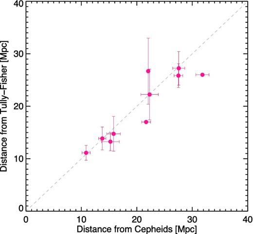
Distances to galaxies having both Tully–Fisher and Cepheids distances. Grey dashed line represents identity. When both measurements are available, a mean distance is calculated considering as many values as possible.
It is crucial that we do not select distances obtained from the SNe Ia studies. As is shown in Moreno-Raya et al. (2016), a discrepancy appears when distances obtained using independent and dependent indicators from SNe Ia are compared. SN Ia techniques provide overestimated distances compared with other methods, and the effect becomes more important at greater distances.
Table 1 shows the sample, sorted by the name of the host galaxies. This table lists the galaxies’ morphology, their redshifts, parallactic angle and semi-axis ratio, introduces as well the SN Ia they host and shows their positions within the galaxies. Distance indicators and distances are also provided.
Galaxies observed at 4.2 m WHT, with their morphology in column 2. Redshifts are given in column 3. Columns 4 and 5 show parallactic angles and ratios between major and minor axis. SNe Ia names are shown in column 6; and their positions, in terms of RA, Dec. offsets and distance in arcsecs from galactic centres, are in columns 7, 8 and 9. PA, b/a and offsets from Asiago SN catalogue. Distance indicators, number of measurements and distance values are shown in columns 10, 11 and 12. Henceforth, data are shown this same order.
| Host galaxy | Morphology | z | PA | b/a | SN Ia | RA offset | Dec. offset | Separation | Distance | Number of | Distance |
|---|---|---|---|---|---|---|---|---|---|---|---|
| (deg) | (arcsec) | (arcsec) | (arcsec) | indicator | measures | (Mpc) | |||||
| M82 | I0 | 0.000 677 | 155 | 0.37 | 2014J | − 54.0 | − 21.0 | 57.9 | PNLF | 6 | 3.8 ± 0.7 |
| MCG-02-16-02 | Sb? | 0.007 388 | 15 | 0.19 | 2003kf | +9.2 | − 14.3 | 17.0 | T-F | 2 | 22.6 ± 0.8 |
| NGC 0105 | Sab: | 0.017 646 | 77 | 0.64 | 1997cw | +7.6 | +4.2 | 8.7 | SN Ia | 6 | 64.2 ± 5.9 |
| NGC 1275 | S0 | 0.017 559 | 20 | 0.64 | 2005mz | +19.2 | − 23.6 | 30.4 | T-F | 2 | 61.4 ± 7.5 |
| NGC 1309 | Sbc: | 0.007 125 | 135 | 0.93 | 2002fk | − 12.0 | − 3.5 | 12.5 | Ceph & T-F | 5 | 29.3 ± 0.9 |
| NGC 2935 | SBb | 0.007 575 | 90 | 0.73 | 1996Z | +0.0 | − 70.0 | 70.0 | T-F | 12 | 28.2 ± 3.2 |
| NGC 3021 | Sbc | 0.005 140 | 20 | 0.56 | 1995al | − 15.0 | +2.9 | 15.3 | Ceph & T-F | 11 | 26.3 ± 1.9 |
| NGC 3147 | Sbc | 0.009 346 | 65 | 0.86 | 1997bq | +50.0 | − 60.0 | 78.1 | T-F | 1 | 40.9 ± 4.1 |
| NGC 3169 | Sa | 0.004 130 | 135 | 0.50 | 2003cg | +14.0 | +5.0 | 14.9 | T-F | 3 | 17.1 ± 2.9 |
| NGC 3368 | Sab | 0.002 992 | 95 | 0.69 | 1998bu | +4.3 | +55.3 | 55.5 | Ceph & T-F | 27 | 11.0 ± 1.0 |
| NGC 3370 | Sc | 0.004 266 | 58 | 0.56 | 1994ae | − 30.3 | +6.1 | 30.9 | Ceph & T-F | 24 | 27.4 ± 1.9 |
| NGC 3672 | Sc | 0.006 211 | 98 | 0.47 | 2007bm | − 2.4 | − 10.8 | 11.1 | T-F | 3 | 22.8 ± 1.8 |
| NGC 3982 | Sb: | 0.003 699 | 90 | 0.87 | 1998aq | − 18.0 | +7.0 | 19.3 | Ceph & T-F | 25 | 21.5 ± 0.8 |
| NGC 4321 | SBbc | 0.005 240 | 120 | 0.81 | 2006X | − 12.0 | − 48.0 | 49.5 | Ceph & T-F | 35 | 15.5 ± 1.9 |
| NGC 4501 | Sb | 0.007 609 | 50 | 0.53 | 1999cl | − 46.0 | +23.0 | 51.4 | T-F | 12 | 20.7 ± 3.2 |
| NGC 4527 | SBbc | 0.005 791 | 157 | 0.33 | 1991T | +26.0 | +45.0 | 52.0 | Ceph & T-F | 21 | 13.8 ± 1.4 |
| NGC 4536 | SBbc | 0.006 031 | 40 | 0.39 | 1981B | +41.0 | +41.0 | 58.0 | Ceph & T-F | 53 | 14.8 ± 1.6 |
| NGC 4639 | SBbc | 0.003 395 | 33 | 0.66 | 1990N | +63.2 | − 1.8 | 63.2 | Ceph & T-F | 44 | 22.3 ± 2.1 |
| NGC 5005 | Sbc | 0.003 156 | 155 | 0.48 | 1996ai | +24.0 | +4.0 | 24.3 | T-F | 4 | 23.2 ± 2.1 |
| NGC 5468 | Scd | 0.009 480 | 15 | 0.91 | 1999cp | − 52.0 | +23.0 | 56.9 | T-F | 1 | 41.5 ± 4.2 |
| NGC 5584 | Scd | 0.005 464 | 50 | 0.72 | 2007af | − 40.0 | − 22.0 | 45.7 | Ceph & T-F | 10 | 24.3 ± 1.3 |
| UGC 00272 | Sd | 0.012 993 | 40 | 0.42 | 2005hk | +17.2 | +6.9 | 18.5 | T-F | 2 | 60.5 ± 3.7 |
| UGC 03218 | Sb | 0.017 432 | 55 | 0.37 | 2006le | − 12.4 | +40.1 | 42.0 | T-F | 4 | 59.0 ± 6.0 |
| UGC 03576 | SBb | 0.019 900 | 38 | 0.54 | 1998ec | − 8.7 | +19.5 | 21.4 | T-F | 5 | 87.4 ± 8.2 |
| UGC 03845 | SBbc | 0.010 120 | 86 | 0.67 | 1997do | − 2.6 | − 3.8 | 4.6 | T-F | 1 | 38.5 ± 3.9 |
| UGC 04195 | SBb | 0.016 305 | 110 | 0.50 | 2000ce | +15.1 | +17.3 | 23.0 | T-F | 4 | 78.8 ± 2.2 |
| UGC 09391 | SBdm | 0.006 384 | 110 | 0.59 | 2003du | − 8.8 | − 13.5 | 16.1 | T-F | 1 | 31.8 ± 3.2 |
| UGCA 017 | Scd: | 0.006 535 | 111 | 0.16 | 1998dm | − 13.8 | − 37.0 | 39.5 | T-F | 13 | 26.3 ± 4.4 |
2.2 Observations
We obtained intermediate-resolution long-slit spectroscopy for all our sample of local SN Ia host galaxies. For this, we used the 4.2 m William Herschel Telescope (WHT), located at the Roque de los Muchachos Observatory (ORM, La Palma, Canary Islands, Spain). We completed two observation runs in 2011 December and 2014 January. In both cases, the double-arm ISIS (Intermediate dispersion Spectrograph and Imaging System) instrument located at the Cassegrain focus was used. The dichroic used to separate the blue and red beams was set at 5400 Å. The slit was 3.7 arcmin long and 1 arcsec wide. As an example, Fig. 2 shows the slit positions over three galaxies. Blue zones correspond to regions with extracted useful spectra, while the location of the SN Ia is represented with a yellow circle. Appendix B provides the same figures for all our sample galaxies.
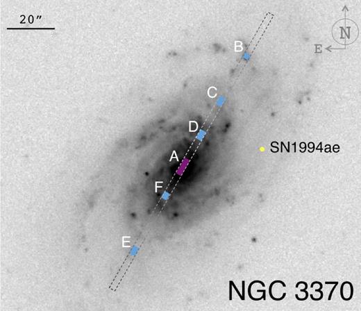
R-band images for NGC 3370 hosting SN1994ae. Slit size is not to scale. Blue zones correspond to regions in which we have obtained spectra, whereas purple zones represent regions without emission lines. SNe Ia positions are marked with a yellow dot. All figures can be seen in Appendix B.
The observational details of each observing run are as follows.
2011 December. We were granted with two observation nights, December 22 and 23, in which we observed 12 galaxies following this set-up:
Blue arm. An EVV CCD with a 4096 × 2048 pixel array and 13.5 μm size was used with a spatial scale of 0.20 arcsec pixel−1. The grating used was the R600B, giving a dispersion of 33 Å mm−1 (0.45 Å pixel−1).
Red arm. We used a REDPLUS CCD with a configuration of 4096 × 2048 pixels of 24 μm pixel size, having a spatial scale of 0.22 arcsec pixel−1. We used the grating R600R, which has a dispersion of 33 Å mm−1 (0.49 Å pixel−1).
Table 2 compiles the different central wavelengths used among these two nights due to the redshift range of the sample, in order to cover the emission lines for the subsequent analysis.
(ii) 2014 January. 16 galaxies were observed during the four nights of this run: from January 23 to 26. We used the same instrumental set-up that for the 2011 December run. However, in this case only one pair of central wavelengths was enough to cover the whole spectral range. The central wavelengths of this configuration and other details are also compiled in Table 2.
Central wavelengths for both the blue and red ISIS arms for the four configurations used in our observations. Identifications z0, z1 and z2 refer to the 2011 December run. z2014 refers to those used for the 2014 January run.
| Configuration | Central λ (Å) | Spectral range λ (Å) | ||
|---|---|---|---|---|
| Blue arm | Red arm | Blue arm | Red arm | |
| z0 | 4368 | 6720 | 3560–5186 | 5892–7538 |
| z1 | 4452 | 6950 | 3652–5284 | 6122–7768 |
| z2 | 4549 | 7023 | 3749–5385 | 6195–7841 |
| z2014 | 4438 | 6783 | 3630–5266 | 5995–7601 |
Arc lamps were used for the wavelength calibration of the spectra. Specifically, the lamps used were ‘CuAr’ for the blue arm, and ‘CuAr+CuNe’ for the red arm. The absolute flux calibration was achieved by observing the standard stars Hiltner 600, HD 19445 and HD 84937 (Stone 1977; Oke & Gunn 1983). Between two and four individual exposures were obtained for each slit position in order to get a good signal-to-noise ratio (SNR) and achieve a proper cosmic ray removal. Table 3 compiles all the intermediate-resolution long-slit spectroscopy observations performed for the 28 SN Ia host galaxies included in this paper.
Instrument specifications for the observations taken at the 4.2 m WHT in both runs. Galaxies are sorted as in Table 1.
| Host galaxy | SN Ia | Date | Exp. time | Spatial R. | Grism | PA | Airmass |
|---|---|---|---|---|---|---|---|
| (s) | (arcsec pixel−1) | (°) | |||||
| M82 | 2014J | 24-Jan-2014 | 3×600 | 0.20 | R600B | 248 | 1.699 358 |
| 24-Jan-2014 | 4×300 | 0.22 | R600R | 248 | 1.703 212 | ||
| MCG-02-16-02 | 2003kf | 24-Jan-2014 | 2×1800 | 0.20 | R600B | 290 | 1.415 056 |
| 24-Jan-2014 | 2×1800 | 0.22 | R600R | 290 | 1.414 584 | ||
| NGC 0105 | 1997cw | 26-Jan-2014 | 2×1800 | 0.20 | R600B | − 6 | 1.358 633 |
| 26-Jan-2014 | 2×1800 | 0.22 | R600R | − 6 | 1.433 069 | ||
| NGC 1275 | 2005mz | 26-Jan-2014 | 2×1800 | 0.20 | R600B | 62 | 1.196 434 |
| 26-Jan-2014 | 2×1800 | 0.22 | R600R | 62 | 1.196 645 | ||
| NGC 1309 | 2002fk | 26-Jan-2014 | 2×1800 | 0.20 | R600B | 28 | 1.487 035 |
| 26-Jan-2014 | 2×1800 | 0.22 | R600R | 28 | 1.487 479 | ||
| NGC 2935 | 1996Z | 25-Jan-2014 | 2×1800 | 0.20 | R600B | 329 | 1.753 246 |
| 25-Jan-2014 | 2×1800 | 0.22 | R600R | 329 | 1.689 944 | ||
| NGC 3021 | 1995al | 22-Dec-2011 | 2×1200 | 0.20 | R600B | 93 | 1.285 784 |
| 22-Dec-2011 | 2×1200 | 0.22 | R600R | 93 | 1.285 847 | ||
| NGC 3147 | 1997bq | 22-Dec-2011 | 2×1200 | 0.20 | R600B | 320 | 1.509 696 |
| 22-Dec-2011 | 2×1200 | 0.22 | R600R | 320 | 1.542 244 | ||
| NGC 3169 | 2003cg | 23-Dec-2011 | 2×1200 | 0.20 | R600B | 172 | 1.262 523 |
| 23-Dec-2011 | 2×1200 | 0.22 | R600R | 172 | 1.295 006 | ||
| NGC 3368 | 1998bu | 24-Jan-2014 | 2×1800 | 0.20 | R600B | 298 | 1.306 252 |
| 24-Jan-2014 | 2×1800 | 0.22 | R600R | 298 | 1.307 326 | ||
| NGC 3370 | 1994ae | 22-Dec-2011 | 2×1800 | 0.20 | R600B | 330 | 1.160 587 |
| 22-Dec-2011 | 2×1800 | 0.22 | R600R | 330 | 1.125 012 | ||
| NGC 3672 | 2007bm | 25-Jan-2014 | 2×1800 | 0.20 | R600B | 364 | 1.497 680 |
| 25-Jan-2014 | 2×1800 | 0.22 | R600R | 364 | 1.498 453 | ||
| NGC 3982 | 1998aq | 24-Jan-2014 | 2×1800 | 0.20 | R600B | 335 | 1.154 017 |
| 24-Jan-2014 | 2×1800 | 0.22 | R600R | 335 | 1.140 907 | ||
| NGC 4321 | 2006X | 22-Dec-2011 | 2×1800 | 0.20 | R600B | 340 | 1.134 375 |
| 22-Dec-2011 | 2×1800 | 0.22 | R600R | 340 | 1.171 063 | ||
| NGC 4501 | 1999cl | 25-Jan-2014 | 2×1800 | 0.20 | R600B | 322 | 1.145 303 |
| 25-Jan-2014 | 3×1800 | 0.22 | R600R | 322 | 1.145 677 | ||
| NGC 5005 | 1996ai | 22-Dec-2011 | 2×1200 | 0.20 | R600B | 250 | 1.080 511 |
| 22-Dec-2011 | 2×1200 | 0.22 | R600R | 250 | 1.096 719 | ||
| NGC 4527 | 1991T | 24-Jan-2014 | 2×1800 | 0.20 | R600B | 64 | 1.266 297 |
| 24-Jan-2014 | 2×1800 | 0.22 | R600R | 64 | 1.317 050 | ||
| NGC 4536 | 1981B | 24-Jan-2014 | 2×1800 | 0.20 | R600B | 265 | 1.663 660 |
| 24-Jan-2014 | 2×1800 | 0.22 | R600R | 265 | 1.666 170 | ||
| NGC 4639 | 1990N | 24-Jan-2014 | 2×1800 | 0.20 | R600B | 335 | 1.060 286 |
| 24-Jan-2014 | 2×1800 | 0.22 | R600R | 335 | 1.077 132 | ||
| NGC 5468 | 1999cp | 26-Jan-2014 | 2×1800 | 0.20 | R600B | 7 | 2.028 415 |
| 26-Jan-2014 | 2×1800 | 0.22 | R600R | 7 | 2.030 882 | ||
| NGC 5584 | 2007af | 25-Jan-2014 | 2×1800 | 0.20 | R600B | 308 | 1.439 699 |
| 25-Jan-2014 | 2×1800 | 0.22 | R600R | 308 | 1.438 900 | ||
| UGC 00272 | 2005hk | 22-Dec-2011 | 4×600 | 0.20 | R600B | 126 | 1.160 984 |
| 22-Dec-2011 | 4×600 | 0.22 | R600R | 126 | 1.158 374 | ||
| UGC 03218 | 2006le | 25-Jan-2014 | 2×1800 | 0.20 | R600B | 142 | 1.200 891 |
| 25-Jan-2014 | 2×1800 | 0.22 | R600R | 142 | 1.200 936 | ||
| UGC 03576 | 1998ec | 25-Jan-2014 | 2×1800 | 0.20 | R600B | 130 | 1.073 760 |
| 25-Jan-2014 | 2×1800 | 0.22 | R600R | 130 | 1.073 590 | ||
| UGC 03845 | 1997do | 26-Jan-2014 | 2×1800 | 0.20 | R600B | 214 | 1.055 408 |
| 26-Jan-2014 | 2×1800 | 0.22 | R600R | 214 | 1.055 376 | ||
| UGC 04195 | 2000ce | 26-Jan-2014 | 2×1800 | 0.20 | R600B | 188 | 1.268 553 |
| 26-Jan-2014 | 2×1800 | 0.22 | R600R | 188 | 1.268 342 | ||
| UGC 09391 | 2003du | 23-Dec-2011 | 3×900 | 0.20 | R600B | 190 | 1.765 348 |
| 23-Dec-2011 | 3×900 | 0.22 | R600R | 190 | 1.810 054 | ||
| UGCA 017 | 1998dm | 23-Dec-2011 | 3×1200 | 0.20 | R600B | 202 | 1.584 673 |
| 23-Dec-2011 | 3×1200 | 0.22 | R600R | 202 | 1.529 884 |
The slit position was fixed independently for each galaxy by looking at the acquisition image. Usually, the slit was orientated following the direction that allowed us to observe the highest number of H ii regions. This orientation does not coincide with the SNe Ia positions, as the SNe Ia neighbourhood usually lacked measurable star formation activity. Hence, we prioritized that position angle (PA) that provides the largest number of H ii regions in order that we could use their data to derive a metallicity gradient for the galaxy.
2.3 Reduction of the spectra
iraf3 software was used to reduce the CCD frames (debiasing, flat-fielding, cosmic ray rejection, wavelength and flux calibration, sky subtraction) and to extract the one-dimensional spectra. Correction for atmospheric extinction was performed using an average curve for the continuous atmospheric extinction at ORM. For each two-dimensional spectrum, several apertures were defined along the spatial direction to extract the final one-dimensional spectra of each galaxy or emission knot. The apertures were centred at the brightest point of each aperture and the width was fixed to obtain a good SNR in each spectrum. In this case, we have the optical spectrum separated in two different wavelength intervals with different spatial resolutions, so it was essential to be precise in order to get identical apertures in both spectral ranges. For the blue arm, Hβ was the reference line to extract these apertures, while in the red arm, Hα was the used line.
Fig. 3 shows a set of spectra for NGC 3370. The main emission line features are identified with labels. The 1D spectra usually have a high SNR for all the lines (e.g. ∼22, and always over 6 for Hβ).
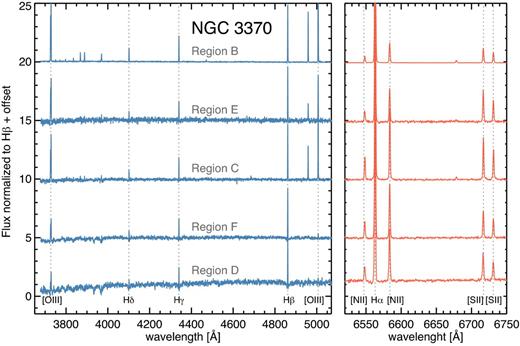
Spectra obtained for the five H ii regions analysed in NGC 3370, as labelled in the top panel of Fig. 2. The main emission lines are identified. Note that the GCD of the H ii regions decreases from top (region B) to bottom (region D).
3 ANALYSIS
3.1 Line measurements
For the 28 galaxies, a total of 102 apertures have been extracted. 13 of these apertures lack measurable emission lines, and hence these have not been included in the subsequent analysis. For the remaining 89 regions, we tried to measure all the emission lines we are interested in. In most of the spectra, we have measured eight emission lines: three hydrogen Balmer lines (Hα, Hβ, Hγ) and the brightest collisional excited lines of metallic elements: [O ii] λλ3726,29 (blended), [O iii] λ5007, [N ii] λ6583, [S ii] λλ6716, 6731. If a line is measured and its SNR ≤ 3, we do not consider it. Line intensities and equivalent widths were measured integrating all the emission between the limits of the line and over a local adjacent continuum. All these measurements were made with the SPLOT routine of iraf. However, due to the faintness of some of the detected emission lines, a detailed inspection of the spectra was needed to get a proper estimation of the adjacent continuum and the line flux in these cases. Uncertainties in the line fluxes were estimated for each line considering both the rms of the continuum and the width of each emission line.
3.2 Correction for reddening
Typical analysis of star-forming regions always consider that the theoretical I(Hα)/I(Hβ) ratio is 2.86, following the case B recombination for an electron temperature of Te = 10 000 K and electron density of ne = 100 cm−2. However, the theoretical H ii Balmer ratios also depend – although weakly – on the electron temperature (Storey & Hummer 1995). Objects with Te ∼ 15 000 K have I(Hα)/I(Hβ) = 2.86, whereas objects with Te ∼ 5000 K have I(Hα)/I(Hβ) = 3.01. These values are also related to the oxygen abundance of the ionized gas, in the sense that objects with higher (lower) electron temperature have lower (higher) oxygen abundances. We have used the prescriptions given by López-Sánchez et al. (2015) – see their appendix B – to consider the electron temperature dependence of the theoretical H i Balmer line ratios assuming the best value to the oxygen abundance provided by the empirical calibrations (see the next subsection).
Appendix A provides the line intensities for the regions which make up the sample. Reddening coefficient is also shown here.
3.3 Nature of the emission
We first check the nature of the ionization of the gas within the regions observed in our sample galaxy. For this, we use the so-called diagnostic or BPT diagrams, first proposed by Baldwin, Phillips & Terlevich (1981) and Veilleux & Osterbrock (1987). These diagrams are excellent tools for distinguishing between active galactic nucleus (AGN) or low-ionization narrow emission-line region (LINER) activity and pure star-forming regions since H ii regions and starburst galaxies lie within a narrow band. Fig. 4 shows the typical BPT diagrams considering [O iii] λ5007/Hβ versus [N ii] λ6583/Hα (top) and [O iii] λ5007/Hβ versus ([S ii] λ6716+λ6731)/Hα (bottom).
![BPT diagrams comparing the observational flux ratio [O iii] λ5007/Hβ (y-axis) with the [N ii] λ6583/Hα (top) and ([S ii] λ6716+λ6731)/Hα (bottom) flux ratios (x-axis) obtained for our galaxy sample. The theoretical line proposed by Kewley et al. (2001) is plotted using a purple continuous line, while the empirical line obtained by Kauffmann et al. (2003) is shown with a pink dashed line. Red circles indicate galaxies classified as AGN, orange circles are the galaxies with composite nature, while blue circles represent pure star-forming galaxies.](https://oup.silverchair-cdn.com/oup/backfile/Content_public/Journal/mnras/462/2/10.1093_mnras_stw1706/2/m_stw1706fig4.jpeg?Expires=1750391858&Signature=E~1uDaPb7kKoilRD5ZfCcfwCuhyaBB0NCcwIjH~a4oLSjk~UmVeYYs~VOSk1KedMWAn0FW2ce1LdWr0lYZLC5e9594FmqRzA7GHsmS~G~xujJ6FReyZgnQkTY4ZFhKOUt1RBwQTSwspmZ1JGSVW6OlnDgQ9S0FSSWeAxRMC3Xp1zN4fH6l6ubfR0gYQbytPnKoETbgjgPmoFFBmOUpjVgXR9YRnnDXp6tM96yNJZGiHjpe7SGLmgTVQjtOugOBycY7nCv-taW486gooe6-66U0X1Z5N0rrheMMLMNSbduWRVL-hTtGRISR5V7SLYSuizNEiBiZSlShzrgiY-YrabUw__&Key-Pair-Id=APKAIE5G5CRDK6RD3PGA)
BPT diagrams comparing the observational flux ratio [O iii] λ5007/Hβ (y-axis) with the [N ii] λ6583/Hα (top) and ([S ii] λ6716+λ6731)/Hα (bottom) flux ratios (x-axis) obtained for our galaxy sample. The theoretical line proposed by Kewley et al. (2001) is plotted using a purple continuous line, while the empirical line obtained by Kauffmann et al. (2003) is shown with a pink dashed line. Red circles indicate galaxies classified as AGN, orange circles are the galaxies with composite nature, while blue circles represent pure star-forming galaxies.
63 of the observed spectra have all the emission lines needed for classifying their nature following BPT diagram; their data points are included in Fig. 4. For the remaining 26 spectra, the [O iii] λ5007/Hβ flux radio was not available, and hence these regions could not be classified following the BPT method. Fig. 4 also includes the analytic relations given by Kewley et al. (2001) – continuous purple line – which were derived for starburst galaxies and which represent an upper envelope of positions of star-forming galaxies.
For regions where the gas is excited by shocks, accretion discs or cooling flows (as is in the case of AGNs or LINERs), their position in these diagnostic diagrams is away from the locus of H ii regions, and usually well above the theoretical Kewley et al. (2001) curves. Hence, the nature of the ionization of the gas within these areas is not due to massive stars, and therefore they cannot be classified as star-forming regions. Data points not classified as H ii regions are coloured in red in Fig. 4 and are not further considered in our analysis. We find only three of these regions, which are therefore classified as AGN. Thus, we have finally classified 60 spectra as coming from star-forming regions.
The top panel of Fig. 4 includes the empirical relation between the [O iii] λ5007/Hβ and the [N ii] λ6583/Hα provided by Kauffmann et al. (2003) – dashed pink line – after analysing a large data sample of star-forming galaxies from Sloan Digital Sky Survey (SDSS) data is also drawn. All galaxies lying below this curve are considered to be pure star-forming objects, and hence are plotted using blue colour in the figure.
Kewley et al. (2006) suggested that those objects between the theoretical line computed by Kewley et al. (2001) and the empirical line found by Kauffmann et al. (2003) may be ionized by both massive stars and shocks, i.e. have a composite nature, although Pérez-Montero & Contini (2009) showed that objects located in this area may also be pure star-forming galaxies with high [N ii] intensities due to a high N content. In these cases, we use orange colour to distinguish these regions, which will also be analysed in our work. All regions classified as AGN in the top panel of Fig. 4 lie above the theoretical curve shown in the bottom panel, too. Similarly, both star-forming and composite objects lie below this curve in the bottom panel, within the errors.
The 26 regions lacking [O iii] λ5007/Hβ could not, obviously, be classified on the basis of these two BPT diagrams. However, we may use the information coming from [N ii]/Hα. The top panel of Fig. 5 shows the distribution of [N ii]/Hα for the 63 regions classified by the diagnostic diagrams. The distribution is split into star-forming (blue), composite (orange) and AGNs (red). Fig. 5 includes the distribution of unclassified regions (purple). All the 26 unclassified regions lie left to the limit defined by our AGNs, and they follow distribution which is equivalent to that observed for the star-forming regions. Besides that, we may look at the spectra: if a region lacks [O iii] λ5007 with Hβ being present, then the ratio log[O iii]/Hβ will be always negative, so its position will be at the bottom part of Fig. 4 and at the left of the minimum value of [N ii]/Hα of our AGNs. In other words: combining the information of the distribution of log([N ii]/Hβ) seen in Fig. 5 and the experience at examining spectra we may consider that these unclassified spectra are actually coming from star-forming regions. Adding these 26 regions to the 60 regions already classified as star-forming, we finally get a sample of 86 pure star-forming regions to be analysed in our study.

N2 and S2 parameter distributions in the measured regions. Dotted line represents an upper limit to differentiate between AGN and SF regions. As all unclassified regions lie above the upper limit, we consider them as SF (composite at least), and we include them in the subsequent analysis.
4 RESULTS
4.1 Chemical abundances using strong emission lines methods
These two indices present some advantages with respect to using other parameters.
Both N2 and O3N2 are not affected by reddening, since the lines involved are so close in wavelength that this effect is cancelled. The reddening correction is important, for example, when considering the R23 or N2O2 parameters (see López-Sánchez & Esteban 2010, for more details)
As the intensity of oxygen lines does not monotonically increase with metallicity, parameters involving oxygen ratios (i.e. R23) are actually bivalued. Again, this does not affect either the N2 nor O3N2 indices. In the case of the R23 parameter, different calibrations must be given for the low – 12 + log(O/H)≲ 8.0 – and the high – 12 + log(O/H)≳ 8.4 – metallicity regimes.
Therefore, it is very convenient to rely on well-behaved parameters, such as N2 or O3N2, to derive the oxygen abundance of the ionized gas in galaxies when auroral lines are not detected, as they do not suffer the problems of the reddening correction nor are bi-valuated. This has been extensively used in the literature in the last decade, although some precautions should still be taken into account when using these parameters (see López-Sánchez et al. 2012). For what refers to those indices used in this work, N2 saturates at high metallicities – 12 + log(O/H)≳8.6 – while O3N2 is not valid in the low-metallicity regime – 12 + log(O/H)≲8.1.
Therefore, we use the above expression to derive OHO3N2 from OHN2 in the 26 regions lacking O3N2 values.
4.2 Radial oxygen abundance distributions
Once the values for OHO3N2 in the 86 H ii regions within our 28 sample galaxies are obtained, we derive the radial distributions of the oxygen abundances and their corresponding radial metallicity gradients for each galaxy. Next we assign a local value of the oxygen abundance at the position of each SN Ia. We proceed as follows.
When several regions within a galaxy have been measured, we derive an abundance radial gradient using a linear fit. If this radial gradient is appropriate (i.e. a good correlation between GCDs and metallicities is measured), we use it to compute the metallicity value for the location of the SN Ia.
If this is not the case, we adopt as metallicity of the SN Ia the oxygen abundance derived in the closest H ii region. This may be caused by two reasons. First, there are not enough points to derive a gradient (usually only one region has been observed within the galaxy, or when only two very nearby regions are observed). Secondly, the dispersion of the data is so high that the derived metallicity gradient does not seem to be real, or it seems highly inaccurate, e.g. when an inverted metallicity gradient (that is considered to be non-realistic in a normal galaxy) is found.
We note that we use the deprojected radial distances for this, a critical measure if we want to assign a proper oxygen abundance value for each region in which the SN is. Deprojecting a galaxy requires two parameters: the PA, which is the angle between the line of nodes of the projected image and the north, and the ratio between the galaxy's axis (b/a) (both parameters are shown in Table 1). If the galaxy is seen face-on, b/a will be 0. Once the deprojected GCD is obtained, we have the metallicity gradient of each galaxy from all observed H ii regions and, this way, we estimate a local abundance for the SNe Ia regions. For that, we assume that both all measured H ii regions and all the SNe Ia are located in the galactic plane.
It is important to remark that we are assuming a unique metallicity radial gradient for each galaxy. In other words, the orientation of the slit does not matter, because the gradient is assumed to be the same in every radial direction. There are not many studies of possible azimuthal variations (but see Sánchez et al. 2015), besides in some few cases when galaxy interactions are observed (e.g. López-Sánchez & Esteban 2009; Bresolin, Kennicutt & Ryan-Weber 2012; López-Sánchez et al. 2015). Azimuthal variations in metallicity could be due to the spiral wave effect or the bar role which may move the gas in a non-asymmetric way and create zones with different elemental abundances even being located at the same GCD. This interesting subject is being studied now with data coming from the on-going Integral Field Spectroscopy (IFS) surveys (Sánchez et al. 2014; Sánchez-Blázquez et al. 2014), as they allow this type of analysis, but it is out of the scope of our work.
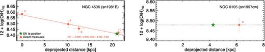
The left-hand panel of Fig. 6 shows a typical abundance radial distribution, where the radial gradient is well determined and have enough points to be sure of the reliability of its slope. Filled points are the values obtained directly with the O3N2 parameter, while open points represent those values of OHO3N2 which have been derived from equation (11). The (red) star marks the position of the SN Ia with the derived value of oxygen abundance. The right-hand panel of Fig. 6 represents a case for which the radial gradient is undefined (in some cases it may be not reliable enough) and for which the value adopted for the SN Ia corresponds to that given by its closest H ii region.
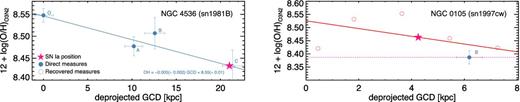
Left: metallicity gradient for NGC 4536. Filled points represent metallicities derived using the O3N2 parameter directly, while open points are those for which the OHO3N2 value was recovered from N2 parameter following equation (11). The blue solid line traces the metallicity gradient, while the pink star represents the SN Ia location with its derived metallicity. Right: for the galaxy NGC 0105, only one H ii region is available (blue circle). We adopt the value (pink star) given by the data from Galbany et al. (2016b, red circles).
To check the consistency of these fits, we also derive all oxygen abundances using the N2 parameter. Fig. 7 shows the abundance radial distributions for the same two galaxies shown in Fig. 6. As we see, the disagreement between both fits is minimal, being identical within the uncertainties. This is further evidence of the robustness of our metallicity values.
Left-hand panel: metallicity gradient for NGC 4536. Red circles represent metallicities derived using the N2 parameter. The orange solid line traces the metallicity gradient, while the green star represents the SN Ia location with its derived metallicity. Right-hand panel: the red circle represents the value of the only H ii region observed in NGC 0105, which is assumed to be the same as all the galaxy (dotted green line). The differences with respect to OHO3N2 are below 0.10 dex.
Appendix B compiles all radial distributions derived for our galaxy sample. We derive accurate metallicity gradients for 21 galaxies, which we use to provide the metallicity of the SN Ia. For the remaining seven galaxies, we use the oxygen abundance value of the closest H ii region as that of the SN Ia. When the distance between the SN Ia and the observed H ii region is larger than 3 kpc, the metallicity of the SN Ia will actually be an upper or a lower limit (depending on the location of the SN Ia with respect to the H ii region). We briefly describe the situation in these seven cases in Appendix B.
Table 4 lists the oxygen abundances for all SN Ia indicating for each case the given value from the radial gradient (if it does exist), the value of the closest region and the final adopted value. We note that values from the closest region and from the gradient are in agreement. A linear fit to the data, which has a correlation coefficient of r = 0.8947, provides a slope of 0.915 ± 0.054 (i.e. very near to 1).
Derived abundances for the environment regions of SNe Ia.
| Host galaxy | SN Ia | OHgradient | OHclosest | OHfinal |
| M82 | 2014J | 8.59 ± 0.15 | 8.58 ± 0.01 | 8.59 ± 0.15 |
| MCG-02-16-02 | 2003kf | 8.38 ± 0.14 | 8.44 ± 0.06 | 8.38 ± 0.14 |
| NGC 0105 | 1997cw | 8.46 ± 0.08a | 8.38 ± 0.02 | 8.46 ± 0.08 |
| NGC 1275 | 2005mz | – | 8.54 ± 0.01 | 8.54 ± 0.01 |
| NGC 1309 | 2002fk | 8.41 ± 0.19 | 8.42 ± 0.04 | 8.41 ± 0.19 |
| NGC 2935 | 1996Z | – | 8.62 ± 0.05 | 8.62 ± 0.05 |
| NGC 3021 | 1995al | 8.57 ± 0.05 | 8.55 ± 0.01 | 8.57 ± 0.05 |
| NGC 3147 | 1997bq | – | 8.66 ± 0.02 | 8.66 ± 0.02 |
| NGC 3169 | 2003cg | 8.75 ± 0.06 | 8.66 ± 0.02 | 8.75 ± 0.06 |
| NGC 3368 | 1998bu | – | 8.51 ± 0.03 | 8.51 ± 0.03 |
| NGC 3370 | 1994ae | 8.30 ± 0.08 | 8.23 ± 0.02 | 8.30 ± 0.08 |
| NGC 3672 | 2007bm | 8.63 ± 0.07 | 8.65 ± 0.05 | 8.63 ± 0.07 |
| NGC 3982 | 1998aq | 8.54 ± 0.05a | 8.58 ± 0.05 | 8.54 ± 0.05 |
| NGC 4321 | 2006X | 8.60 ± 0.12 | 8.59 ± 0.01 | 8.60 ± 0.12 |
| NGC 4501 | 1999cl | 8.43 ± 0.22 | 8.43 ± 0.03 | 8.43 ± 0.22 |
| NGC 4527 | 1991T | 8.50 ± 0.08 | 8.54 ± 0.05 | 8.50 ± 0.08 |
| NGC 4536 | 1981B | 8.43 ± 0.06 | 8.43 ± 0.06 | 8.43 ± 0.06 |
| NGC 4639 | 1990N | 8.16 ± 0.20 | 8.40 ± 0.03 | 8.16 ± 0.20 |
| NGC 5005 | 1996ai | 8.60 ± 0.08 | 8.60 ± 0.01 | 8.60 ± 0.08 |
| NGC 5468 | 1999cp | 8.23 ± 0.08 | 8.32 ± 0.02 | 8.23 ± 0.08 |
| NGC 5584 | 2007af | 8.34 ± 0.08 | 8.47 ± 0.02 | 8.34 ± 0.08 |
| UGC 00272 | 2005hk | 8.25 ± 0.12 | 8.30 ± 0.04 | 8.25 ± 0.12 |
| UGC 03218 | 2006le | 8.59 ± 0.09 | 8.59 ± 0.05 | 8.59 ± 0.09 |
| UGC 03576 | 1998ec | 8.57 ± 0.16 | 8.58 ± 0.06 | 8.57 ± 0.16 |
| UGC 03845 | 1997do | 8.49 ± 0.04 | 8.54 ± 0.01 | 8.49 ± 0.04 |
| UGC 04195 | 2000ce | 8.46 ± 0.05a | 8.57 ± 0.02 | 8.46 ± 0.05 |
| UGC 09391 | 2003du | 8.27 ± 0.10 | 8.31 ± 0.07 | 8.27 ± 0.10 |
| UGCA 017 | 1998dm | 8.32 ± 0.07 | 8.29 ± 0.04 | 8.32 ± 0.07 |
aGradients obtained from Galbany et al. (2016b).
It is important to take into account potential biases introduced by the difference between SN Ia progenitor metallicity (ZIa) at the time of its formation and the metallicity of the host galaxy (ZHOST) measured after the explosion. Bravo & Badenes (2011) presented a theoretical study concluding that SN Ia progenitor metallicity can be reasonably estimated by the host galaxy metallicity, and that is better represented by the gas-phase than the stellar host metallicity. In addition, quoting these authors: ‘for active galaxies, the dispersion of ZIa is quite small, meaning that ZHOST is a quite good estimator of the SN metallicity, while passive galaxies present a larger dispersion’. On the other hand, Galbany et al. (2016b) found that the gas-phase metallicity at the locations of a sample of SNe Ia observed with IFS is on average 0.03 dex higher than the total galaxy metallicity in the MAR13 scale. The differences between local and global stellar metallicities are not significant for SNe Ia, and this enables the use of the environmental metallicity as a proxy for the SN Ia progenitor metallicity.
4.3 Comparing with other results
The metallicities of two galaxies of our sample, NGC 4321 and NGC 4501, were studied by Pilyugin et al. (2002) using the R2 and R23 parameters and the empirical calibration provided by Pilyugin (2001). Fig. 8 compares the gradients for both galaxies derived by these authors with those found in this work. As we can see, the abundances derived by Pilyugin et al. (2002) are systematically higher than those derived here. Such a difference is mainly due to the use of different empirical calibrations. Indeed, the new empirical calibrations derived by MAR13 make it very difficult to get 12 + log (O/H) ≥ 8.69, values which are easily reached by the empirical calibration derived by Pilyugin (2001). As a second cross-check, we have gathered data from McCall, Rybski & Shields (1985), Shields, Skillman & Kennicutt (1991) and Skillman et al. (1996) to get the original emission line fluxes for these two galaxies and we have applied MAR13 calibrations. Fig. 8 also shows in red the gradients obtained with MAR13 calibration. They are in agreement with our results. That stresses the discrepancy between calibrations.
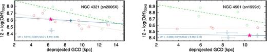
Metallicity gradients for NGC 4321(left) and NGC 4501(right). Symbols are the same as in Fig. 6, except for the open green circles, which represent values from Pilyugin et al. (2002) and the dashed green line, being the gradient that these authors derived from these points. Red points correspond to abundances obtained applying MAR13 calibration to the original data gathered from McCall et al. (1985), Shields et al. (1991) and Skillman et al. (1996), and the red dotted line is the linear fit to the data.
On the other hand, three galaxies for which we have not derived a metallicity gradient (NGC 0105, NGC 3982 and UGC 04195) have been recently observed as part of an extended CALIFA programme. The analysis of these data, presented in Galbany et al. (2016b), provides a metallicity gradient for each of these galaxies which is made up of approximately ∼1000 spectra. For these three galaxies, we were not able to obtain metallicity gradients, so we took the values given in Galbany et al. (2016b), which help us to improve the quality of the data (see Table 4 and Appendix B for more details).
4.4 SN Ia LC parameters
We have gathered LC data for these SNe Ia from different sources (listed in Table 5). These data have been fitted with SiFTO (Conley et al. 2008) to obtain both the LC stretch and the colour. SiFTO is a powerful and versatile LC fitter that manipulates spectral templates to simultaneously match the multi-band photometric data of a particular SN with heliocentric redshift zhel. A stretch parametrization is used to describe the shape of the LC. The SiFTO colour, C, is obtained adjusting the spectral energy distribution to observed colours corrected for Milky Way (MW) extinction with values from Schlafly & Finkbeiner (2011). See González-Gaitán et al. (2014) for a detailed procedure of how we obtain s and C. The LC stretch is defined in the B band.
SNe Ia parameters. From columns 3 to 6: apparent magnitude corrected for MW extinction, colour, stretch and derived absolute magnitudes, respectively. Column 7 shows environment oxygen abundances. SN Ia classes are shown in column 8: 1 for normal SNe Ia, 2 for reddened SNe Ia and 3 for subluminous SNe Ia. Sources for SNe Ia parameters are listed in column 9.
| Host galaxy | SN Ia | mB | C | s | MB | OH | Class | Source |
| M82 | 2014J | 11.332 ± 0.056 | 1.167 ± 0.0090 | 1.070 ± 0.004 | − 16.567 ± 0.056 | 8.59 ± 0.07 | 2 | Marion et al. (2015); Foley et al. (2014); Tsvetkov et al. (2014) |
| MCG-02-16-02 | 2003kf | 13.238 ± 0.132 | − 0.027 ± 0.0490 | 1.055 ± 0.013 | − 18.528 ± 0.132 | 8.44 ± 0.13 | 1 | Hicken et al. (2009) |
| NGC 0105 | 1997cw | 15.939 ± 0.057 | 0.348 ± 0.0240 | 1.105 ± 0.031 | − 18.099 ± 0.057 | 8.39 ± 0.03 | 2 | Jha et al. (2006) |
| NGC 1275 | 2005mz | 16.434 ± 0.067 | 0.325 ± 0.0180 | 0.644 ± 0.006 | − 17.507 ± 0.067 | 8.55 ± 0.03 | 3 | Hicken et al. (2009) |
| NGC 1309 | 2002fk | 13.147 ± 0.018 | − 0.175 ± 0.0200 | 1.013 ± 0.005 | − 19.186 ± 0.018 | 8.38 ± 0.11 | 1 | Hicken et al. (2009) |
| NGC 2935 | 1996Z | 14.348 ± 0.095 | 0.315 ± 0.0230 | 0.915 ± 0.085 | − 17.903 ± 0.095 | 8.62 ± 0.05 | 2 | Riess et al. (1999) |
| NGC 3021 | 1995al | 13.310 ± 0.017 | 0.097 ± 0.0200 | 1.074 ± 0.025 | − 18.789 ± 0.017 | 8.58 ± 0.06 | 1 | Riess et al. (1999) |
| NGC 3147 | 1997bq | 14.388 ± 0.024 | 0.080 ± 0.0180 | 0.917 ± 0.010 | − 18.671 ± 0.024 | 8.66 ± 0.02 | 1 | Jha et al. (2006) |
| NGC 3169 | 2003cg | 15.798 ± 0.014 | 1.154 ± 0.0100 | 0.983 ± 0.004 | − 15.363 ± 0.014 | 8.75 ± 0.06 | 2 | Elias-Rosa et al. (2006); Ganeshalingam et al. (2010); Hicken et al. (2009) |
| NGC 3368 | 1998bu | 12.106 ± 0.013 | 0.267 ± 0.0090 | 0.973 ± 0.009 | − 18.091 ± 0.013 | 8.51 ± 0.03 | 2 | Suntzeff et al. (1999) |
| NGC 3370 | 1994ae | 12.948 ± 0.019 | − 0.079 ± 0.0130 | 1.054 ± 0.008 | − 19.244 ± 0.019 | 8.30 ± 0.08 | 1 | Altavilla et al. (2004); Riess et al. (2005) |
| NGC 3672 | 2007bm | 14.411 ± 0.210 | 0.474 ± 0.0130 | 0.938 ± 0.005 | − 17.379 ± 0.210 | 8.64 ± 0.08 | 2 | Hicken et al. (2009); Stritzinger et al. (2011) |
| NGC 3982 | 1998aq | 12.320 ± 0.009 | − 0.133 ± 0.0080 | 0.986 ± 0.005 | − 19.340 ± 0.009 | 8.59 ± 0.06 | 1 | Riess et al. (2005) |
| NGC 4321 | 2006X | 15.373 ± 0.016 | 1.393 ± 0.0170 | 1.000 ± 0.003 | − 15.572 ± 0.016 | 8.61 ± 0.06 | 2 | Ganeshalingam et al. (2010) |
| NGC 4501 | 1999cl | 14.891 ± 0.017 | 1.129 ± 0.0100 | 0.939 ± 0.008 | − 16.687 ± 0.017 | 8.44 ± 0.12 | 2 | Ganeshalingam et al. (2010); Jha et al. (2006); Krisciunas et al. (2006) |
| NGC 4527 | 1991T | 11.491 ± 0.023 | 0.050 ± 0.0210 | 1.068 ± 0.011 | − 19.210 ± 0.023 | 8.50 ± 0.08 | 1 | Altavilla et al. (2004); Ford et al. (1993); Lira et al. (1998) |
| NGC 4536 | 1981B | – | – | – | – | 8.43 ± 0.06 | 1 | – |
| NGC 4639 | 1990N | 12.675 ± 0.015 | 0.020 ± 0.0110 | 1.064 ± 0.008 | − 19.066 ± 0.015 | 8.17 ± 0.08 | 1 | Lira et al. (1998) |
| NGC 5005 | 1996ai | 16.892 ± 0.012 | 1.676 ± 0.0140 | 1.097 ± 0.024 | − 14.931 ± 0.012 | 8.60 ± 0.09 | 2 | Riess et al. (1999) |
| NGC 5468 | 1999cp | 13.933 ± 0.011 | − 0.047 ± 0.0070 | 0.994 ± 0.006 | − 19.157 ± 0.011 | 8.23 ± 0.08 | 1 | Ganeshalingam et al. (2010); Krisciunas et al. (2000) |
| NGC 5584 | 2007af | 13.156 ± 0.087 | 0.058 ± 0.0130 | 0.970 ± 0.003 | − 18.976 ± 0.087 | 8.34 ± 0.09 | 1 | Hicken et al. (2009); Stritzinger et al. (2011) |
| UGC 00272 | 2005hk | 15.891 ± 0.011 | 0.293 ± 0.0180 | 0.867 ± 0.003 | − 18.018 ± 0.011 | 8.26 ± 0.10 | 3 | Hicken et al. (2009); McCully et al. (2014); Phillips et al. (2007) |
| UGC 03218 | 2006le | 14.751 ± 0.168 | − 0.133 ± 0.0440 | 1.074 ± 0.005 | − 19.104 ± 0.168 | 8.60 ± 0.07 | 1 | Hicken et al. (2009) |
| UGC 03576 | 1998ec | 16.189 ± 0.053 | 0.176 ± 0.0220 | 0.997 ± 0.033 | − 18.518 ± 0.053 | 8.57 ± 0.08 | 1 | Ganeshalingam et al. (2010); Jha et al. (2006) |
| UGC 03845 | 1997do | 14.288 ± 0.037 | 0.019 ± 0.0200 | 0.975 ± 0.020 | − 18.639 ± 0.037 | 8.50 ± 0.04 | 1 | Jha et al. (2006) |
| UGC 04195 | 2000ce | 17.038 ± 0.038 | 0.495 ± 0.0170 | 1.038 ± 0.026 | − 17.445 ± 0.038 | 8.57 ± 0.02 | 2 | Jha et al. (2006); Krisciunas et al. (2001) |
| UGC 09391 | 2003du | 13.462 ± 0.007 | − 0.145 ± 0.0140 | 1.023 ± 0.004 | − 19.050 ± 0.007 | 8.28 ± 0.11 | 1 | Anupama, Sahu & Jose (2005), Hicken et al. (2009); Leonard et al. (2005) |
| UGCA 017 | 1998dm | 14.663 ± 0.020 | 0.264 ± 0.0090 | 1.044 ± 0.006 | − 17.434 ± 0.020 | 8.33 ± 0.08 | 3 | Ganeshalingam et al. (2010); Jha et al. (2006) |
We classify SNe Ia regarding their colour (C) in this way: if C < 0.2, we label them normal SNe; if C > 0.2, we consider they are reddened SNe Ia. Those SNe Ia that have C < 0.2 and a extremely low luminosity (considering that the SN Ia is no reddened) are labelled as subluminous SNe Ia. For the subsequent analysis, subluminous SNe Ia are no longer considered in our study, since their behaviour cannot be explained as the rest of normal SNe Ia.
4.5 Absolute magnitudes
We note that the mB determined by SiFTO is already corrected by the MW extinction, and any contribution of the extinction of the host galaxy as well as intrinsic colour variations is retained in the C SiFTO parameter. Correcting for SN host galaxy extinction is a complicated issue highly debated specially in SN cosmological studies, due to the difficulty to estimate its magnitude. Many assumptions have to be done in order to get proper estimations, including extinction laws, different RV than the standard 3.1 in the MW, etc. However, if the SN Ia is located in the outer parts of the host galaxy, the extinction of its host galaxy seems to be negligible (Galbany et al. 2012), meaning that correcting for MW extinction is enough for our purposes. This can be checked by looking at the colour of the SNe Ia.
Table 5 provides a summary of the measurements presented in this subsection. Column 1 lists the name of the galaxy, while the identification of each SN Ia is shown in column 2. The next three columns list the parameters given by SiFTO (SN peak apparent magnitude, colour C and stretch s). In column 4, we give MB, computed considering only SN Ia independent distance indicators (see Section 2.1). Column 5 compiles the oxygen abundance we derived for each SN Ia location. Column 7 lists the sources for each SN LC photometry.
5 DISCUSSION
In this section, we analyse the absolute magnitudes of SNe Ia in their maximum of the LC, MB and their relation with the oxygen abundances. We also analyse these results in the context of the SNe Ia parameters as their colours and their LC shape.
5.1 Covariance matrix: MB − C − OH − s
In some traditional methods, only two parameters have been considered for reducing the systematics in the SNe Ia distance modulus, i.e. SN colour and LC stretch. They have been used to correct MB, which is considered fixed for all SNe Ia. Here we want to check if the environmental properties of the host galaxies may affect the SNe Ia luminosities. One such property is the metallicity, using the gas-phase oxygen abundance as its proxy. Our first analysis of this study was already presented in Moreno-Raya et al. (2016), where we discussed the metallicity dependence of the MB of the SN Ia for non-reddened objects, i.e. those with C < 0.2, to avoid possible biases with the SN Ia colour. We found that, for those non-reddened SNe Ia, a metallicity dependence does appear when plotting MB as a function of OHO3N2, in the sense that metal-rich galaxies host less luminous SNe Ia than metal-poor galaxies, which host brightest SN Ia. We now want to check if this metallicity dependence is still found when the whole galaxy sample is considered. Hence, we seek to find the relationship between all these parameters. To do this, we perform a PCA, calculating the covariance matrix involving these four parameters following this order: the SNe Ia absolute magnitude (MB), the SNe Ia colour (C), the SNe Ia environment metallicity (OH) and the SNe Ia LC stretch (s).
The elements on the principal diagonal represent the correlation of each parameter with itself, which is always equal to 1. The crossed terms in the covariance matrix indicate how well two parameters are correlated, and have values ranging from 1 to −1. We label the matrix elements in equation (13) as an, m, being n the row in the matrix and m the column. Hence, element, i.e. a4, 3, corresponds to the element placed in the fourth row and the third column, which relates s with OH.
The first row, corresponding to MB, gives us that colour (in the second column) is the most influential parameter, as a1, 2 = 0.9749 [as a2, 1, not shown in equation (13) since the matrix is symmetric]. The terms a1, 3 = 0.5464 and a1, 4 = −0.0222 relate MB with OH and s, respectively. Negative values imply that the parameters are inversely correlated. One can see that none of these terms are negligible. In addition, metallicity correlates with MB almost twice than the LC stretch does. The non-zero values of a1, 3 let us consider to quantify this effect with metallicity.
The value a1, 4 = −0.0222 gives information about the low dispersion of s within the sample. In fact, in our sample, s goes from 0.9 to 1.1, which is a narrow range compared to the reported values in the literature (between 0.4 and 1.6). Thus, the low correlation between MB and s must be taken with caution. On the other hand, 70 per cent of the total SNe Ia population is within this short range (Sullivan et al. 2006). Therefore, a no correlation between s and OH within this range and a possible correlation between them for a wider range of s values may be interesting and significant by itself, although we let this study for a next work.
5.2 MB versus colour
As we discussed in Moreno-Raya et al. (2016), we found that metal-rich galaxies host fainter SNe Ia than those exploding in metal-poor galaxies. This metallicity dependence of the SN Ia luminosity could be attributed to the colour correction, a term already included in the cosmological methods to estimate the distance modulus (and implicitly in the determination of the MB of each SN Ia). Actually, the colour of SNe Ia shows a dependence on the oxygen abundance (as it is seen in covariance matrix). And our data show a good correlation between SNe Ia magnitudes and their colours, as we show in Fig. 9.
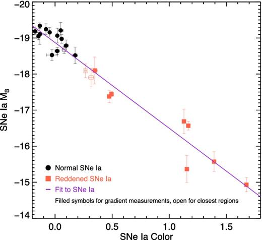
SNe Ia absolute magnitudes, MB, as a function of SNe Ia colour C. Black circles are ‘normal’ SNe Ia and red squares are reddened SNe Ia. The purple line represents a linear fit to all SNe Ia. Open symbols indicate objects for which their metallicities were adopted from a proper gradient estimation, whereas open symbols show objects for which the metallicity was assumed to be the same as the nearest H ii region.
Both fitting parameters, MB = −18.87 and β = 2.38, are in agreement with those reported by Betoule et al. (2014). We note that the dispersion in MB without the colour effect (that should be MB − βC, being β the slope in equation 14) is reduced when it is compared with that shown by the distribution of MB.
5.3 Relation between metallicity and colour
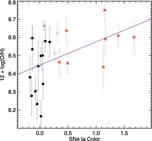
Oxygen abundance as a function of SNe Ia colour. Symbols are the same as in Fig. 9.
As we do not want to consider twice the colour dependence, we create a linear combination between colour and OH which is orthogonal to C. The new orthogonal parameter is OHpure = OH − δ × C, where δ is the slope in equation (15). The correlation coefficient between C and OHpure is r = 0.00641.
5.4 MB − βC versus metallicity
Since a1, 3 is non-zero in the covariance matrix, we should expect that a metallicity dependence does exist. Fig. 11 compares MB − βC (y-axis) with the oxygen abundance (OHpure on the x-axis), showing that, indeed, MB − βC becomes fainter when the metallicity increases. This result agrees with the trend we reported in Moreno-Raya et al. (2016), which claims that metal-rich galaxies host fainter SNe Ia than those observed in metal-poor galaxies.
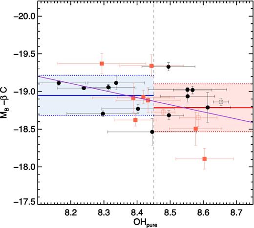
SNe Ia absolute magnitude MB without the colour effect (MB − βC) as a function of oxygen abundance OHO3N2. Symbols are the same as in Fig. 9. The blue and red horizontal solid lines provide the averaged value in the low- and high-metallicity regimes, respectively, with their 1σ uncertainty shown with the pale blue and red areas.
We divide the abundances into low-metallicity, OHO3N2 < 8.45 with MB = −18.95 ± 0.27 mag, and high-metallicity, OHO3N2 > 8.45 with MB = −18.78 ± 0.32 mag, regimes (blue and red horizontal lines in Fig. 11) resulting in a shift of ∼0.17 mag. This result agrees with the shift of 0.14 mag in MB for unreddened SNe Ia found in Moreno-Raya et al. (2016), with high- (low-) metallicity galaxies hosting less (more) luminous SNe Ia. This result depends in part on the faintest object in Fig. 11, SN2003cg (around −18 mag). The two brightest reddened SNe Ia (around −19.4 in the same figure) have also an effect. These three SNe Ia are reddened objects; however, we have already demonstrated that the non-reddened SNe Ia show a significant correlation between MB and OH. In addition, one can see at first glance in this figure that taking only the reddened SNe Ia, a correlation with OH already exists. Therefore, even with caution, we think that dependence on OH is clear, without any reason to discard one or more points.
5.5 MB − βC − γ(OHpure − 8.45) versus stretch
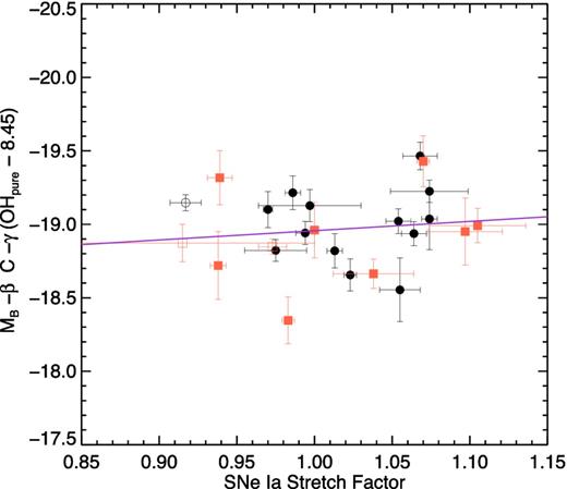
SNe Ia absolute magnitude as a function of LC stretch, as s − 1. Symbols are the same as in Fig. 9.
With this last step, we have decreased further the dispersion of the data. Fig. 13 shows the distribution of magnitudes having been subtracted from traditional parameters (grey filled distribution) compared to the distribution obtained after eliminating the three dependences (colour, LC stretch and metallicity – blue distribution).
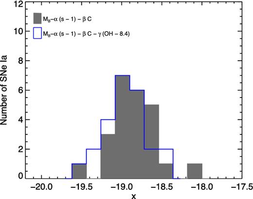
Histogram showing the distribution for MB, labelled as x in the horizontal axis, with C and s dependence subtraction (grey) and removing as well metallicity dependence (blue).
The standard deviation in our sample in the latter case is now reduced by a factor of 5.1 per cent when compared with the standard deviation computed when only the two traditional parameters (colour and LC stretch) are considered. Therefore, including the metallicity dependence in the analysis eliminates a small, but measurable, luminosity scatter. This result implies a possible improvement in reducing the Hubble residuals when using SN Ia techniques.
We have proven how independent measurements of MB depend on these three parameters: C, s and OHpure. A forthcoming paper will include a proper cosmological analysis taking into account all these parameters at the same time.
6 CONCLUSIONS
We present an analysis of the gas-phase oxygen abundances for 28 galaxies that have experienced a SN Ia event. We used intermediate-resolution long-slit spectroscopy obtained at the 4.2 m WHT to derive reliable oxygen abundances of H ii regions within the host galaxies. SNe Ia absolute magnitudes have been calculated with parameters given by modern techniques, such SALT2. We seek for a possible dependence of the SNe Ia luminosities on the metallicity of the regions where exploded. Below we summarize the main conclusions found in our analysis.
We applied the most recent empirical calibrations by MAR13, which involve the N2 and O3N2 indices and are appropriate for measuring oxygen abundances in well-defined H ii regions, to obtain consistent abundance radial distributions and their corresponding gradient, with which proper oxygen abundances for the locations within their host galaxies where SNe Ia exploded are estimated. This is important, since we have obtained local values of oxygen abundance for each SN Ia, instead of what in the literature has been done before, assuming a global metallicity from a unique spectrum (which means a centre region abundance estimate) or, even worst, through the use of a mass–metallicity relation. Our technique improves by ∼0.2 dex the accuracy of the oxygen abundances determined in SN Ia host galaxies.
In our analysis, we consider both normal and reddened SNe Ia, and analysed the colour effect over the MB. That is an improvement of the results found in Moreno-Raya et al. (2016), where we only used normal (i.e. non-reddened) SNe Ia.
We demonstrate that the effect of the metallicity cannot be neglected in SN Ia studies that use their magnitudes, MB, or distance moduli, μ, since its dependence on the oxygen abundance does not have a zero value in the covariance matrix. This correction appears as a second-order correction after the colour correction, since, for our sample, the dependence on LC stretch is low.
Our conclusions agree with those presented in Moreno-Raya et al. (2016), where fainter SNe Ia are found to exist in metal-rich galaxies, whereas brightest SNe Ia occur in galaxies with a poor content in metals when a subsample of non-reddened objects was used. Hubble residuals measured using the common SNe Ia standardization technique (colour and stretch corrections) are found to be correlated to the metal abundance of their host galaxies, in the direction of SNe Ia where metal-rich galaxies are brighter, implying an overcorrection on those objects. Our results show that this overcorrection may be interpreted as a metallicity dependence which has not been taken into account in the standardization.
We strongly claim, for our local sample, that including the oxygen abundance dependence the dispersion in MB is reduced to around 5 per cent. Therefore, we agree with Campbell, Fraser & Gilmore (2016) that using the metallicity as a third parameter might help to reduce the systematic dispersion in cosmological studies of SNe Ia. This possibility will be checked in a future work (Moreno-Raya et al., in preparation) extending the redshift range of the galaxy sample from the local Universe presented here.
This is a step forward compared to the existing studies so far. In a near future, it will be possible to perform more detailed analysis using IFS data (Galbany et al. 2014, 2016a,b).
The metallicity dependence found in this paper may well be important for present and future SN cosmology surveys, helping to minimize the scatter on the SN HD. This could be achieved by considering extra parameters in the LC fitting or distance modulus calculations.
We acknowledge the anonymous referee for his/her helpful comments. We thank Miguel Cárdenas-Montes, Santiago González-Gaitán, Inma Domínguez and Brad Gibson for their inestimable comments and help. Based on observations made with the 4.2 m WHT operated on the islands of La Palma by the Isaac Newton Group of Telescopes in the Spanish observatory of Roque de Los Muchachos of the Instituto de Astrofísica de Canarias. MEMR thanks the hospitality of the staff at both the Australian Astronomical Observatory (Australia) and Departamento de Astronomía of the Universidad de Chile (Chile) during his stay in 2013 and 2014, respectively. ARL-S thanks the support of the ‘Study of Emission-Line Galaxies with Integral-Field Spectroscopy’ (SELGIFS) programme, funded by the EU (FP7-PEOPLE-2013-IRSES-612701). This work has been partially supported by MINECO-FEDER grant AYA2010-21887-C04-02 and AYA2013-47742-C4-4-P. Support for LG is provided by the Ministry of Economy, Development, and Tourism's Millennium Science Initiative through grant IC120009 awarded to the Millennium Institute of Astrophysics (MAS), and CONICYT through FONDECYT grant 3140566. ACR acknowledges financial support provided by the PAPDRJ CAPE/FAPERJ Fellowship. This research has made use of the NASA/IPAC Extragalactic Database (NED) which is operated by the Jet Propulsion Laboratory, California Institute of Technology, under contract with the National Aeronautics and Space Administration.
Here we use the terms metallicity, total abundance in metals, Z (being X + Y + Z = 1 in mass) and oxygen abundances indistinctly, assuming that log (Z/Z⊙) = log (O/H) − log (O/H)⊙, 12 + log (O/H)⊙ = 8.69 and Z⊙ = 0.019 being the solar values (Asplund et al. 2009).
Image Reduction Analysis Facility, distributed by the National Optical Astronomy Observatories (NOAO), which is operated by AURA Inc., under cooperative agreement with NSF.
It is important to note that a distinction has to be made when deriving oxygen abundances from resolved H ii regions and from galaxies (i.e. spectra from the SDSS or the Galaxy And Mass Assembly survey). Each situation requires the proper empirical calibration, since integrated galaxy spectra do not consider only the pure H ii regions but the whole galaxy. In those cases, some aperture corrections must be taken into account (Iglesias-Páramo et al. 2013).
REFERENCES
APPENDIX A: LINE INTENSITIES
This appendix provides Table A1, which gives line intensities for the sample spectra. All intensities are given over I(Hβ) except those labelled with a, in which spectra there were no Hβ emission lines measurable. In these cases, the provided intensities are over I(Hα).
Extinction coefficients and de-reddened intensities for the sample. All intensities are over I(Hβ). For those regions where I(Hβ) was not available, intensities are over I(Hα).
| Galaxy | Region | c(Hβ) | I([O ii]) | I(Hγ) | I(Hβ) | I([O iii]) | I(Hα) | I([N ii]) | I([S ii]) | I([S ii]) |
|---|---|---|---|---|---|---|---|---|---|---|
| λ3727 | λ4340 | λ4861 | λ5007 | λ6563 | λ6584 | λ6717 | λ6731 | |||
| M82 | A | 1.93 ± 0.01 | – | 0.67 ± 0.01 | 1.00 ± 0.01 | 0.31 ± 0.01 | 2.86 ± 0.02 | 1.52 ± 0.01 | 0.29 ± 0.03 | 0.33 ± 0.03 |
| M82 | B | 2.22 ± 0.01 | – | 0.67 ± 0.03 | 1.00 ± 0.01 | 0.27 ± 0.01 | 2.86 ± 0.05 | 1.53 ± 0.03 | 0.28 ± 0.01 | 0.31 ± 0.01 |
| MCG-02-16-02 | B | 0.60 ± 0.16 | – | – | 1.00 ± 0.16 | 2.05 ± 0.50 | 2.86 ± 0.67 | 0.28 ± 0.07 | 0.31 ± 0.08 | 0.22 ± 0.06 |
| MCG-02-16-02 | C | 0.58 ± 0.12 | – | – | 1.00 ± 0.14 | 2.51 ± 0.50 | 2.86 ± 0.03 | 0.21 ± 0.02 | 0.18 ± 0.03 | 0.09 ± 0.06 |
| NGC 0105 | A | 0.52 ± 0.14 | – | – | 1.00 ± 0.14 | 9.03 ± 1.77 | 2.86 ± 0.56 | 3.98 ± 0.78 | 0.87 ± 0.18 | 0.85 ± 0.18 |
| NGC 0105 | B | 0.34 ± 0.02 | – | 0.28 ± 0.03 | 1.00 ± 0.02 | 1.27 ± 0.04 | 2.86 ± 0.09 | 0.77 ± 0.02 | 0.47 ± 0.02 | 0.31 ± 0.01 |
| NGC 0105 | C | 0.94 ± 0.06 | – | – | 1.00 ± 0.06 | 4.25 ± 0.39 | 2.86 ± 0.26 | 0.15 ± 0.02 | 0.29 ± 0.03 | 0.22 ± 0.02 |
| NGC 1275 | C | 0.02 ± 0.04 | – | 0.34 ± 0.04 | 1.00 ± 0.04 | 0.65 ± 0.04 | 2.86 ± 0.15 | 2.19 ± 0.11 | 0.51 ± 0.03 | 0.32 ± 0.02 |
| NGC 1309 | B | 0.17 ± 0.01 | 2.38 ± 0.04 | 0.43 ± 0.01 | 1.00 ± 0.01 | 0.73 ± 0.01 | 2.86 ± 0.03 | 0.66 ± 0.01 | 0.51 ± 0.01 | 0.36 ± 0.03 |
| NGC 1309 | B+C | 0.35 ± 0.01 | 2.23 ± 0.04 | 0.44 ± 0.01 | 1.00 ± 0.01 | 0.78 ± 0.01 | 2.86 ± 0.02 | 0.63 ± 0.01 | 0.48 ± 0.03 | 0.35 ± 0.03 |
| NGC 1309 | C | 0.34 ± 0.01 | 1.56 ± 0.04 | 0.44 ± 0.01 | 1.00 ± 0.01 | 0.89 ± 0.01 | 2.86 ± 0.03 | 0.56 ± 0.01 | 0.42 ± 0.03 | 0.28 ± 0.03 |
| NGC 1309 | D | 0.23 ± 0.04 | 2.28 ± 0.25 | 0.50 ± 0.07 | 1.00 ± 0.04 | 0.57 ± 0.05 | 2.86 ± 0.18 | 0.85 ± 0.05 | 0.63 ± 0.04 | 0.48 ± 0.03 |
| NGC 2935 | A | 1.15 ± 0.10 | – | – | 1.00 ± 0.10 | 2.43 ± 0.38 | 2.86 ± 0.42 | 2.76 ± 0.40 | 0.76 ± 0.11 | 0.75 ± 0.11 |
| NGC 2935a | C | – | – | – | – | – | 1.00 ± 0.02 | 0.37 ± 0.06 | – | – |
| NGC 2935a | D | – | – | – | – | – | 1.00 ± 0.08 | 0.45 ± 0.11 | 0.29 ± 0.24 | – |
| NGC 2935a | E | – | – | – | – | – | 1.00 ± 0.04 | 0.46 ± 0.08 | – | – |
| NGC 3021 | B | 0.53 ± 0.01 | 0.96 ± 0.08 | 0.50 ± 0.02 | 1.00 ± 0.01 | 0.16 ± 0.02 | 2.86 ± 0.06 | 1.07 ± 0.02 | 0.40 ± 0.01 | 0.30 ± 0.01 |
| NGC 3021 | C | 0.54 ± 0.02 | 1.34 ± 0.05 | 0.56 ± 0.03 | 1.00 ± 0.02 | 0.26 ± 0.02 | 2.86 ± 0.07 | 1.07 ± 0.03 | 0.46 ± 0.01 | 0.33 ± 0.01 |
| NGC 3021 | D | 0.00 ± 0.01 | 0.62 ± 0.05 | 0.35 ± 0.02 | 1.00 ± 0.01 | 0.29 ± 0.02 | 2.86 ± 0.06 | 1.01 ± 0.02 | 0.50 ± 0.01 | 0.35 ± 0.01 |
| NGC 3021 | E | 0.68 ± 0.03 | 1.80 ± 0.28 | 0.35 ± 0.06 | 1.00 ± 0.03 | 0.19 ± 0.03 | 2.86 ± 0.13 | 1.02 ± 0.05 | 0.45 ± 0.03 | 0.33 ± 0.02 |
| NGC 3147 | B | 0.25 ± 0.03 | – | 0.45 ± 0.03 | 1.00 ± 0.03 | 0.06 ± 0.02 | 2.86 ± 0.10 | 0.76 ± 0.03 | 0.27 ± 0.01 | 0.19 ± 0.01 |
| NGC 3147 | C | 0.55 ± 0.06 | – | – | 1.00 ± 0.06 | 0.16 ± 0.02 | 2.86 ± 0.24 | 0.74 ± 0.07 | 0.18 ± 0.04 | 0.23 ± 0.05 |
| NGC 3147 | D | 1.03 ± 0.16 | – | – | 1.00 ± 0.16 | – | 2.86 ± 0.65 | 1.03 ± 0.24 | 0.29 ± 0.08 | 0.23 ± 0.06 |
| NGC 3147 | E | 0.65 ± 0.05 | – | – | 1.00 ± 0.05 | – | 2.86 ± 0.21 | 0.59 ± 0.05 | 0.17 ± 0.03 | 0.13 ± 0.03 |
| NGC 3169 | E | 0.00 ± 0.02 | 2.22 ± 0.06 | 0.41 ± 0.02 | 1.00 ± 0.02 | 1.31 ± 0.04 | 2.86 ± 0.07 | 0.85 ± 0.02 | 0.44 ± 0.01 | 0.31 ± 0.01 |
| NGC 3169 | G | 0.34 ± 0.08 | – | – | 1.00 ± 0.08 | 0.09 ± 0.03 | 2.86 ± 0.33 | 1.13 ± 0.13 | 0.48 ± 0.06 | 0.36 ± 0.06 |
| NGC 3368 | B | 0.32 ± 0.01 | – | 0.45 ± 0.02 | 1.00 ± 0.01 | 0.14 ± 0.01 | 2.86 ± 0.06 | 1.00 ± 0.02 | 0.46 ± 0.01 | 0.32 ± 0.01 |
| NGC 3368 | C | 0.52 ± 0.12 | – | – | 1.00 ± 0.12 | – | 2.86 ± 0.48 | 0.80 ± 0.14 | 0.50 ± 0.08 | 0.32 ± 0.06 |
| NGC 3370 | B | 0.17 ± 0.03 | 2.03 ± 0.02 | 0.49 ± 0.03 | 1.00 ± 0.03 | 2.59 ± 0.01 | 2.86 ± 0.01 | 0.29 ± 0.03 | 0.22 ± 0.03 | 0.16 ± 0.03 |
| NGC 3370 | C | 0.46 ± 0.01 | 1.97 ± 0.08 | 0.42 ± 0.01 | 1.00 ± 0.01 | 1.67 ± 0.03 | 2.86 ± 0.04 | 0.81 ± 0.01 | 0.51 ± 0.01 | 0.39 ± 0.01 |
| NGC 3370 | D | 0.21 ± 0.03 | – | 0.43 ± 0.03 | 1.00 ± 0.03 | 0.18 ± 0.05 | 2.86 ± 0.11 | 0.95 ± 0.04 | 0.47 ± 0.02 | 0.35 ± 0.02 |
| NGC 3370 | E | 0.07 ± 0.02 | 1.67 ± 0.09 | 0.39 ± 0.02 | 1.00 ± 0.02 | 0.87 ± 0.03 | 2.86 ± 0.09 | 0.62 ± 0.02 | 0.55 ± 0.02 | 0.36 ± 0.01 |
| NGC 3370 | F | 0.41 ± 0.01 | 0.96 ± 0.11 | 0.49 ± 0.02 | 1.00 ± 0.01 | 0.11 ± 0.02 | 2.86 ± 0.05 | 0.78 ± 0.02 | 0.39 ± 0.01 | 0.28 ± 0.01 |
| NGC 3672 | A | 0.84 ± 0.03 | – | 0.72 ± 0.07 | 1.00 ± 0.03 | 0.16 ± 0.03 | 2.86 ± 0.11 | 0.90 ± 0.04 | 0.35 ± 0.01 | 0.27 ± 0.01 |
| NGC 3672 | O | 1.04 ± 0.14 | – | – | 1.00 ± 0.14 | – | 2.86 ± 0.56 | 1.41 ± 0.29 | 0.46 ± 0.11 | 0.32 ± 0.08 |
| NGC 3672a | B | – | – | – | – | – | 1.00 ± 0.01 | 0.37 ± 0.02 | 0.17 ± 0.04 | 0.12 ± 0.06 |
| NGC 3982 | A | 0.95 ± 0.05 | – | – | 1.00 ± 0.05 | 17.38 ± 1.30 | 2.86 ± 0.21 | 3.33 ± 0.25 | 0.78 ± 0.06 | 1.10 ± 0.08 |
| NGC 3982 | B | 0.41 ± 0.02 | – | 0.34 ± 0.03 | 1.00 ± 0.02 | 0.12 ± 0.02 | 2.86 ± 0.07 | 0.95 ± 0.02 | 0.20 ± 0.01 | 0.15 ± 0.01 |
| NGC 3982 | C | 0.34 ± 0.02 | – | 0.37 ± 0.02 | 1.00 ± 0.02 | 0.09 ± 0.01 | 2.86 ± 0.08 | 1.03 ± 0.03 | 0.41 ± 0.01 | 0.29 ± 0.01 |
| NGC 3982 | D | 0.45 ± 0.01 | – | 0.48 ± 0.02 | 1.00 ± 0.01 | 0.23 ± 0.04 | 2.86 ± 0.05 | 0.84 ± 0.02 | 0.39 ± 0.01 | 0.29 ± 0.01 |
| NGC 3982a | E | – | – | – | – | – | 1.00 ± 0.03 | 0.38 ± 0.01 | 0.13 ± 0.01 | 0.09 ± 0.02 |
| NGC 4321 | B | 0.43 ± 0.01 | 0.51 ± 0.07 | 0.42 ± 0.02 | 1.00 ± 0.01 | 0.14 ± 0.02 | 2.86 ± 0.04 | 0.75 ± 0.01 | 0.35 ± 0.01 | 0.26 ± 0.01 |
| NGC 4321 | C | 0.36 ± 0.03 | – | 0.47 ± 0.05 | 1.00 ± 0.03 | – | 2.86 ± 0.13 | 0.61 ± 0.03 | 0.20 ± 0.02 | 0.15 ± 0.02 |
| NGC 4321 | E | 1.05 ± 0.04 | – | 0.64 ± 0.07 | 1.00 ± 0.04 | – | 2.86 ± 0.15 | 0.97 ± 0.05 | 0.31 ± 0.02 | 0.23 ± 0.02 |
| NGC 4501 | B | 0.97 ± 0.12 | – | – | 1.00 ± 0.12 | – | 2.86 ± 0.47 | 0.50 ± 0.09 | 0.18 ± 0.04 | 0.16 ± 0.03 |
| NGC 4501 | C | 0.94 ± 0.10 | – | – | 1.00 ± 0.10 | – | 2.86 ± 0.42 | 0.69 ± 0.10 | 0.21 ± 0.04 | 0.18 ± 0.04 |
| NGC 4501a | A | – | – | – | – | – | 1.00 ± 0.01 | 0.21 ± 0.05 | 0.06 ± 0.16 | 0.07 ± 0.20 |
| NGC 4527 | A | 1.13 ± 0.07 | – | – | 1.00 ± 0.07 | 0.41 ± 0.12 | 2.86 ± 0.28 | 1.01 ± 0.10 | 0.45 ± 0.05 | 0.32 ± 0.03 |
| NGC 4527 | B | 0.72 ± 0.06 | – | – | 1.00 ± 0.06 | 0.26 ± 0.08 | 2.86 ± 0.24 | 1.04 ± 0.09 | 0.45 ± 0.05 | 0.38 ± 0.04 |
| NGC 4527 | D | 1.08 ± 0.06 | – | – | 1.00 ± 0.06 | – | 2.86 ± 0.22 | 0.96 ± 0.08 | 0.32 ± 0.03 | 0.25 ± 0.02 |
| NGC 4527 | E | 0.89 ± 0.15 | – | – | 1.00 ± 0.15 | – | 2.86 ± 0.62 | 0.85 ± 0.19 | 0.39 ± 0.09 | 0.24 ± 0.05 |
| NGC 4527a | F | – | – | – | – | – | 1.00 ± 0.02 | 0.32 ± 0.06 | – | – |
| NGC 4527a | O | – | – | – | – | – | 1.00 ± 0.03 | 0.53 ± 0.01 | 0.17 ± 0.03 | 0.13 ± 0.03 |
| NGC 4536 | A | 0.60 ± 0.04 | – | 0.49 ± 0.07 | 1.00 ± 0.04 | 0.51 ± 0.05 | 2.86 ± 0.18 | 0.83 ± 0.05 | 0.51 ± 0.03 | 0.36 ± 0.02 |
| NGC 4536 | B | 0.33 ± 0.07 | – | – | 1.00 ± 0.07 | 0.31 ± 0.20 | 2.86 ± 0.29 | 0.69 ± 0.08 | 0.54 ± 0.07 | 0.36 ± 0.05 |
| NGC 4536 | O | 1.33 ± 0.02 | – | 0.56 ± 0.03 | 1.00 ± 0.02 | 0.35 ± 0.02 | 2.86 ± 0.06 | 1.27 ± 0.03 | 0.55 ± 0.01 | 0.45 ± 0.01 |
| NGC 4536a | C | – | – | – | – | – | 1.00 ± 0.02 | 0.20 ± 0.05 | 0.22 ± 0.07 | 0.17 ± 0.11 |
| NGC 4639 | A | 0.23 ± 0.02 | – | 0.45 ± 0.02 | 1.00 ± 0.02 | 0.20 ± 0.02 | 2.86 ± 0.06 | 0.94 ± 0.02 | 0.41 ± 0.04 | 0.30 ± 0.01 |
| NGC 4639 | B | 0.21 ± 0.06 | – | – | 1.00 ± 0.05 | 0.27 ± 0.08 | 2.86 ± 0.23 | 1.04 ± 0.09 | 0.30 ± 0.05 | 0.24 ± 0.04 |
| NGC 4639 | C | 0.45 ± 0.07 | – | – | 1.00 ± 0.07 | 1.18 ± 0.16 | 2.86 ± 0.28 | 0.90 ± 0.10 | – | – |
| NGC 5005 | A | 0.46 ± 0.01 | 0.51 ± 0.07 | 0.44 ± 0.02 | 1.00 ± 0.01 | 0.10 ± 0.03 | 2.86 ± 0.05 | 0.75 ± 0.02 | 0.32 ± 0.01 | 0.23 ± 0.01 |
| NGC 5005 | B | 0.78 ± 0.02 | 0.99 ± 0.10 | 0.44 ± 0.03 | 1.00 ± 0.02 | 0.15 ± 0.02 | 2.86 ± 0.06 | 1.00 ± 0.02 | 0.35 ± 0.01 | 0.26 ± 0.01 |
| NGC 5468 | A | 0.04 ± 0.01 | – | 0.37 ± 0.02 | 1.00 ± 0.01 | 0.14 ± 0.02 | 2.86 ± 0.05 | 1.06 ± 0.02 | 0.47 ± 0.01 | 0.38 ± 0.01 |
| NGC 5468 | B | 0.00 ± 0.01 | 1.93 ± 0.03 | 0.43 ± 0.01 | 1.00 ± 0.01 | 2.25 ± 0.03 | 2.86 ± 0.03 | 0.31 ± 0.01 | 0.37 ± 0.01 | 0.26 ± 0.01 |
| NGC 5468 | C | 0.07 ± 0.01 | 1.84 ± 0.05 | 0.45 ± 0.01 | 1.00 ± 0.01 | 1.41 ± 0.02 | 2.86 ± 0.03 | 0.45 ± 0.01 | 0.42 ± 0.01 | 0.29 ± 0.01 |
| NGC 5584 | A | 0.07 ± 0.04 | – | – | 1.00 ± 0.04 | 0.44 ± 0.04 | 2.86 ± 0.16 | 0.69 ± 0.04 | 0.51 ± 0.03 | 0.29 ± 0.02 |
| NGC 5584 | B | 0.24 ± 0.09 | – | – | 1.00 ± 0.09 | 0.46 ± 0.10 | 2.86 ± 0.37 | 0.68 ± 0.09 | – | – |
| NGC 5584 | C | 0.31 ± 0.12 | – | – | 1.00 ± 0.12 | 0.90 ± 0.17 | 2.86 ± 0.48 | 0.57 ± 0.10 | 0.47 ± 0.09 | 0.35 ± 0.07 |
| NGC 5584 | O | 0.15 ± 0.08 | – | – | 1.00 ± 0.08 | 0.19 ± 0.06 | 2.86 ± 0.33 | 0.92 ± 0.11 | 0.56 ± 0.07 | 0.41 ± 0.06 |
| UGC 00272 | A | 0.18 ± 0.04 | – | 0.53 ± 0.08 | 1.00 ± 0.04 | 0.84 ± 0.08 | 2.86 ± 0.18 | 0.88 ± 0.06 | 0.80 ± 0.05 | 0.62 ± 0.04 |
| UGC 00272 | C | 0.04 ± 0.05 | – | – | 1.00 ± 0.05 | 0.69 ± 0.07 | 2.86 ± 0.21 | 0.59 ± 0.06 | 0.71 ± 0.06 | 0.48 ± 0.04 |
| UGC 00272 | D | 1.30 ± 0.13 | – | 0.83 ± 0.23 | 1.00 ± 0.12 | 1.50 ± 0.28 | 2.86 ± 0.51 | 0.50 ± 0.11 | 0.64 ± 0.12 | 0.46 ± 0.09 |
| UGC 00272 | F | 0.00 ± 0.08 | – | – | 1.00 ± 0.07 | 1.50 ± 0.18 | 2.86 ± 0.31 | 0.35 ± 0.06 | 0.60 ± 0.09 | 0.49 ± 0.08 |
| UGC 03218a | A | – | – | – | – | – | 1.00 ± 0.03 | 0.40 ± 0.09 | – | – |
| UGC 03218a | B | – | – | – | – | – | 1.00 ± 0.03 | 0.39 ± 0.06 | 0.30 ± 0.12 | 0.20 ± 0.18 |
| UGC 03218a | O | – | – | – | – | – | 1.00 ± 0.01 | 0.37 ± 0.03 | 0.14 ± 0.05 | 0.09 ± 0.06 |
| UGC 03576a | A | – | – | – | – | – | 1.00 ± 0.02 | 0.39 ± 0.05 | 0.20 ± 0.09 | 0.15 ± 0.10 |
| UGC 03576a | C | – | – | – | – | – | 1.00 ± 0.03 | 0.47 ± 0.03 | – | – |
| UGC 03576a | D | – | – | – | – | – | 1.00 ± 0.04 | 0.39 ± 0.09 | – | – |
| UGC 03845 | A | 0.39 ± 0.04 | – | – | 1.00 ± 0.04 | 0.30 ± 0.05 | 2.86 ± 0.18 | 0.99 ± 0.06 | 0.59 ± 0.04 | 0.45 ± 0.03 |
| UGC 03845 | B | 0.33 ± 0.01 | 3.23 ± 0.10 | 0.03 ± 0.01 | 1.00 ± 0.03 | 0.11 ± 0.02 | 2.86 ± 0.09 | 0.53 ± 0.01 | 0.49 ± 0.01 | 0.36 ± 0.01 |
| UGC 04195 | A | 0.42 ± 0.05 | – | 0.40 ± 0.07 | 1.00 ± 0.05 | 0.34 ± 0.06 | 2.86 ± 0.22 | 1.48 ± 0.11 | 0.40 ± 0.03 | 0.38 ± 0.03 |
| UGC 09391 | A | 0.41 ± 0.03 | 0.72 ± 0.12 | 0.31 ± 0.04 | 1.00 ± 0.03 | 2.55 ± 0.10 | 2.86 ± 0.11 | 0.24 ± 0.01 | 0.41 ± 0.03 | 0.28 ± 0.02 |
| UGC 09391 | B | 0.63 ± 0.09 | 2.23 ± 0.49 | – | 1.00 ± 0.09 | 0.93 ± 0.14 | 2.86 ± 0.36 | 0.32 ± 0.05 | 0.50 ± 0.07 | 0.36 ± 0.05 |
| UGC 09391 | C | 0.37 ± 0.08 | 1.69 ± 0.36 | – | 1.00 ± 0.08 | 1.00 ± 0.13 | 2.86 ± 0.32 | 0.57 ± 0.07 | 0.61 ± 0.07 | 0.44 ± 0.06 |
| UGC 09391 | D | 0.72 ± 0.21 | 9.46 ± 2.96 | – | 1.00 ± 0.21 | 1.52 ± 0.47 | 2.86 ± 0.84 | 0.42 ± 0.13 | 0.75 ± 0.22 | 0.53 ± 0.16 |
| UGCA 017 | A | 0.60 ± 0.07 | – | – | 1.00 ± 0.07 | 2.38 ± 0.24 | 2.86 ± 0.27 | 0.29 ± 0.04 | 0.30 ± 0.04 | 0.21 ± 0.03 |
| UGCA 017 | B | 0.45 ± 0.04 | 1.11 ± 0.21 | 0.30 ± 0.04 | 1.00 ± 0.04 | 1.37 ± 0.09 | 2.86 ± 0.17 | 0.39 ± 0.02 | 0.50 ± 0.03 | 0.36 ± 0.02 |
| UGCA 017 | C | 0.49 ± 0.04 | 2.22 ± 0.49 | 0.39 ± 0.06 | 1.00 ± 0.04 | 1.03 ± 0.07 | 2.86 ± 0.16 | 0.67 ± 0.04 | 0.72 ± 0.04 | 0.53 ± 0.03 |
| UGCA 017 | D | 0.40 ± 0.02 | 1.53 ± 0.12 | 0.36 ± 0.03 | 1.00 ± 0.02 | 0.93 ± 0.03 | 2.86 ± 0.08 | 0.66 ± 0.02 | 0.54 ± 0.02 | 0.38 ± 0.01 |
| UGCA 017 | E | 0.70 ± 0.07 | 5.89 ± 0.65 | – | 1.00 ± 0.07 | 2.04 ± 0.21 | 2.86 ± 0.29 | 0.47 ± 0.05 | 0.60 ± 0.07 | 0.43 ± 0.05 |
aDue to the lack of Hβ, intensities are over I(Hα).
APPENDIX B: GALAXY GRADIENTS
This appendix compiles both the images and the metallicity measurements of all the 28 galaxies included in this paper (Figs B1, B2, B3, B4, B5, B6 and B7). Figures are made up of two panels. The left-hand panels show the R-band image for the galaxy with the slit position (the slit position is not to scale). The position of the SN Ia is marked with a yellow circle. Observed regions are represented within the slit; each one has been identified with a capital letter. The regions are drawn in different colours depending on the nature of the emission: blue for star-forming regions, yellow for composite, red for AGNs and purple for regions without emission lines. The right-hand panels show the oxygen abundance as a function of the GCD. The H ii regions for which oxygen abundances are derived are plotted using blue circles. A pink star marks the position and metallicity for each SN Ia. Metallicity gradients (continuous blue line) are shown when they have been derived. Symbols are the same as in Fig. 6.
Here we describe as well the situation in the seven conflicting cases where a metallicity gradient could not be obtained.
NGC 0105. Only one region is measured at a distance of 2 kpc from the position of the SN Ia. Since there is a proper metallicity gradient given by Galbany et al. (2016b), we adopt that value for the oxygen abundance in the environment of SN1997cw (see the third panel in Fig. B1).
NGC 1275. Only one region is measured at a distance of ∼3.5 kpc from the position of the SN Ia (see the bottom panel in Fig. B1).
UGC 04195. Only one region is measured at a distance of ∼ 8 kpc from the SN Ia position. In this case, there is a proper metallicity gradient available in Galbany et al. (2016b), so we adopt that value for the oxygen abundance in the environment of SN2000ce (see Fig. B7, second panel).
NGC 2935. Three H ii regions are measured in this object, but the gradient is not reliable. All points here have been recovered from N2 parameter. The closest H ii region to the SN Ia is at a distance of ∼ 3 kpc (see the second panel in Fig. B2).
NGC 3147. Data for four H ii regions are available, but the derived metallicity gradient is very steep and inverted. We do not consider this metallicity gradient to be representative, so we adopt the metallicity of the SN Ia as that derived in the closest H ii region, which is located at a distance of 7 kpc. Therefore, the assigned value actually is an upper limit to the real metallicity of the SN Ia, as the latter one is located at a larger galactocentric radius than the measured H ii region (Fig. B2, bottom panel).
(vi)NGC 3368. Data for two H ii regions providing very similar metallicities are available, but they are located at both sides of the galaxy centre and at almost the same GCD, ∼1 kpc, and hence the gradient is not representative. Furthermore, the SN Ia lies very close to one of these H ii regions, so it is easily acceptable that both share the same metallicity (Fig. B3, third panel).
NGC 3982. Data of four H ii regions provide a very steep inverted metallicity gradient, which are not considered to be real. In this case, a proper metallicity gradient is obtained in Galbany et al. (2016b), so that we can adopt that value for the oxygen abundance in the environment of SN1998aq (first panel in Fig. B4).
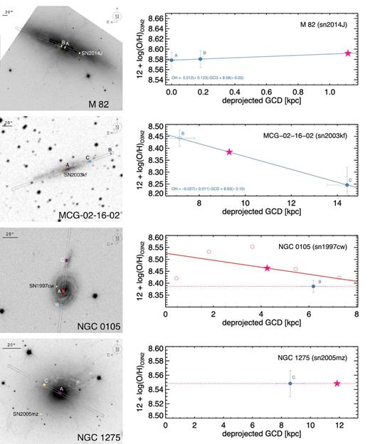
Set of galaxies with extracted regions and derived gradients (or closest regions).
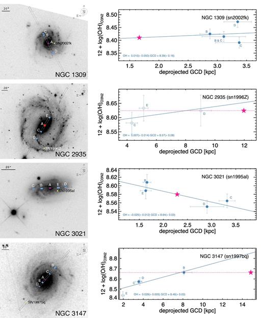
Set of galaxies with extracted regions and derived gradients (or closest regions).
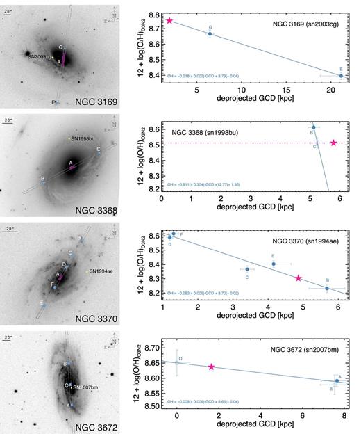
Set of galaxies with extracted regions and derived gradients (or closest regions).
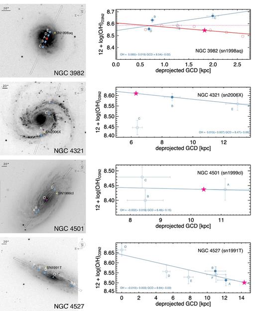
Set of galaxies with extracted regions and derived gradients (or closest regions).
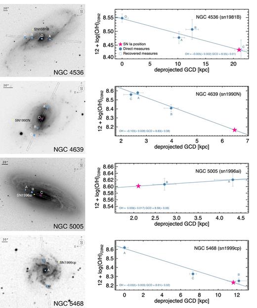
Set of galaxies with extracted regions and derived gradients (or closest regions).
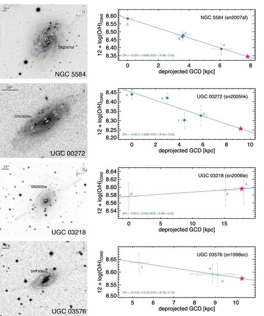
Set of galaxies with extracted regions and derived gradients (or closest regions).
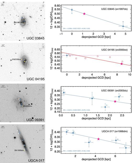
Set of galaxies with extracted regions and derived gradients (or closest regions).
