


Abstract
Galaxies arrive on the red sequences of clusters at high redshift (z > 1) once their star formation is quenched and evolve passively thereafter. However, we have previously found that cluster red sequence galaxies (CRSGs) undergo significant morphological evolution subsequent to the cessation of star formation, at some point in the past 9–10 Gyr. Through a detailed study of a large sample of cluster red sequence galaxies spanning 0.2 < z < 1.4 we elucidate the details of this evolution. Below z ∼ 0.5–0.6 (in the last 5–6 Gyr) there is little or no morphological evolution in the population as a whole, unlike in the previous 4–5 Gyr. Over this earlier time (i) disc-like systems with Sérsic n < 2 progressively disappear, as (ii) the range of their axial ratios similarly decreases, removing the most elongated systems (those consistent with thin discs seen at an appreciable inclination angle) and (iii) radial colour gradients (bluer outwards) decrease in an absolute sense from significant age-related gradients to a residual level consistent with the metallicity-induced gradients seen in low-redshift cluster members. The distribution of their effective radii shows some evidence of evolution, consistent with growth of at most a factor <1.5 between z ∼ 1.4 and ∼0.5, significantly less than for comparable field galaxies, while the distribution of their central (<1 kpc) bulge surface densities shows no evolution at least at z < 1. A simple model involving the fading and thickening of a disc component after comparatively recent quenching (after z ∼ 1.5) around an otherwise passively evolving older spheroid component is consistent with all of these findings.
1 INTRODUCTION
An advantage of studying the cluster galaxy population to test theories of galaxy formation is that, once a galaxy has entered a cluster, it will likely remain within a high-density environment. We can therefore trace a more direct evolutionary connection between high redshift and local systems without needing to appeal to abundance matching to link populations at different epochs (e.g. Guo et al. 2010 et seq.), where the large intrinsic scatter in galaxy growth rates in simulations implies that one cannot unambiguously identify galaxy progenitors and descendants between different observational epochs in the field (Torrey et al. 2015). The homogeneity of cluster samples offers a snapshot of galaxy properties at each epoch, providing a more direct link between galaxy progenitors and descendants. For this reason, cluster galaxies may serve as an important benchmark for models of galaxy formation and evolution, as well as being useful cosmological probes.
The most distinctive and characteristic population of cluster galaxies at z < 1 are the cluster red sequence galaxies (CRSGs). They form such a distinctive population that their colours can be used to search for high-redshift clusters in wide-field images (e.g. Gladders & Yee 2000; Eisenhardt et al. 2008). These predominantly early-type galaxies have little or no ongoing star formation subsequent to forming the bulk of their stellar populations and assembling their stellar masses at high redshift (e.g. Kodama & Arimoto 1997; Stanford, Eisenhardt & Dickinson 1998; De Propris et al. 1999; Mancone et al. 2010; Mei et al. 2012 and references herein). However, while their stellar populations and luminosities evolve passively, their morphologies may not, and may also evolve differently from those of similarly passive field galaxies.
For example, a population of dense and compact quiescent galaxies has been identified in the field at high redshift and appears to be much less common nearer the present epoch (e.g. Taylor et al. 2010; Newman et al. 2012; McLure et al. 2013; Damjanov et al. 2014). Cluster early-type galaxies instead appear to have larger sizes than a similarly massive sample of quiescent field galaxies (Cerulo et al. 2014; Delaye et al. 2014) and to evolve more slowly (Kelkar et al. 2015). Galaxy size evolution may also have significant environmental dependencies (Lani et al. 2013; Damjanov et al. 2015). In our previous study (De Propris, Bremer & Phillipps 2015, hereafter Paper I), we explored the morphologies of a sample of CRSGs drawn from four rich clusters at 1 < z < 1.4 (mean redshift z ∼ 1.25). We used deep archival Hubble Space Telescope (HST) imaging in the rest-frame B- and R-bands (observed frame F850W and F160W). The latter passband probes the evolution of structural parameters in a rest-frame band more representative of the stellar mass distribution (as opposed to earlier studies where the equivalent bandpasses are closer to U or B). Our data implied even weaker size evolution than previously measured (e.g. Cerulo et al. 2014; Delaye et al. 2014) with no significant size growth compared to the Virgo Cluster.
While we confirmed the essentially passive evolution of CRSGs in colour and luminosity, we also observed that a typical CRSG (with a luminosity around L* or fainter) in these z ∼ 1.25 clusters has a considerably more disc-like morphology (lower Sérsic index, more flattened light distribution) than its present-day counterparts, structurally closer to that of field spirals. In agreement with this, Papovich et al. (2012) also measured more oblate shapes for CRSGs in a z = 1.62 cluster partly included within the Cosmic Assembly Near-infrared Deep Extragalactic Legacy Survey (CANDELS) data set, and argued for the presence of increasingly important disc-like components in high-redshift cluster galaxies. In the field, luminous quiescent galaxies also appear to contain significant disc-like components (Bundy et al. 2010; Bruce et al. 2012, 2014; Buitrago et al. 2013), with at least some of these systems showing evidence of being rotationally supported (Buitrago et al. 2014).
One possible clue to the mechanisms that convert these high-redshift ‘discs’ to the more spheroid-dominated population of more local clusters is offered by the existence of significant radial colour gradients. Local early-type galaxies tend to show slightly bluer colours outwards, consistent with the existence of a metal abundance gradient (e.g. Saglia et al. 2000; Tamura & Ohta 2000). Based on the measured colour gradients of La Barbera et al. (2003) it appears that cluster galaxies are already similar to local early-type galaxies in this respect by z = 0.6. Our sample in Paper I showed significantly larger gradients (also bluer outwards) at z = 1.3, more consistent with the existence of age gradients and more similar to the evolution seen by La Barbera et al. (2003) in their sample of discs. Together with the evidence for disc-like components and more flattened shapes (e.g. Papovich et al. 2012; see fig. 7 in Paper I), we argued in Paper I that a population of recently quenched thin discs transforms into the local population of CRSGs (dominated by E/S0 galaxies) largely by mechanisms that do not change stellar mass (given the observed passive evolution of the luminosity function) or overall sizes (as those of our sample were broadly consistent with local values as measured in the Virgo Cluster). Possible mechanisms that give rise to these morphological changes include minor mergers, harassment, fly-bys and tidal effects, among many others.
These objects may also be related to the red spirals found locally in the outskirts of the A901/2 supercluster by Wolf et al. (2009) and in Sloan Digital Sky Survey (SDSS) clusters by Skibba et al. (2009) and Masters et al. (2010). Such ‘anaemic’ spirals with weak spiral structure and low star formation rates were originally identified by van den Bergh (1976) and Koopmann & Kenney (1998) in the Virgo Cluster. These objects may represent the low-redshift counterparts of our high-redshift CRSGs with significant disc components, and would argue that a process of transformation from field-like spirals to cluster E/S0 may have been taking place in a similar fashion across the past 2/3 of the Hubble time. This also suggests that most CRSGs may contain residual discs, a hypothesis supported by earlier photometric work of Michard (1994) and the recent ATLAS3D dynamical work (Emsellem et al. 2007; Krajnovic et al. 2008).
Here we extend this analysis by bridging the intervening redshift range with the full sample of clusters in the Cluster Lensing And Supernova survey with Hubble (CLASH) HST data set (Postman et al. 2012). Thanks to the multiband nature of CLASH, we are able to select our targets in the same way as the targets in Paper I, i.e. by rest-frame R-band luminosity and B − R colour. As before, we also measure structural parameters in (rest frame) R and colour gradients in B − R. We can therefore choose objects over similar magnitude ranges and with very similar stellar populations at all redshifts (tied by the observed passive evolution in both quantities) and measure them in the same fashion as our higher redshift galaxies in Paper I. This yields a comprehensive survey of CRSG structural evolution for objects brighter than ∼ M* + 2 (where M* is the magnitude corresponding to L* in the luminosity function), over the last ∼9–10 Gyr, drawn from a broad sample of clusters, treated in a uniform manner across redshift (as regards to object selection, use of the same passbands and style of analysis).
We discuss the data set and our analysis in the next section. Results including photometry (in AB system, unless otherwise stated), measurements of sizes, Sérsic indices, ellipticities and colour gradients are presented in Section 3. The results are discussed and placed in context via a simple evolutionary model in Section 4. Conclusions are presented in Section 5. Throughout this paper we assume a cosmology based on the latest release of parameters from 9-year Wilkinson Microwave Anisotropy Probe (WMAP9; Hinshaw et al. 2013).
2 DATA SET
The sample of clusters from which all our CRSGs are drawn consists of all available systems targeted in the multiwavelength CLASH Treasury Project1 (Postman et al. 2012). We supplement this with four high-redshift clusters (XMM 1229 – Santos et al. 2009; RDCS 1252 – Rosati et al. 2004; ISCS 1434 – Eisenhardt et al. 2008 and XMM 2235 – Rosati et al. 2009) with suitable archival data at 0.98 < z < 1.40 as already discussed in Paper I. See Table 1 for basic information. The small number of higher redshift objects in our sample is due to the lack (at present) of suitable infrared imaging data sets for z > 0.8 clusters in the HST archive.
Clusters studied in this paper split into the four redshift-dependent groups discussed in the text.
| Cluster | Redshift | |
|---|---|---|
| Abell 383 | 0.187 | Low |
| Abell 209 | 0.206 | |
| Abell 1423 | 0.213 | |
| Abell 2261 | 0.224 | |
| RX 2129+0005 | 0.234 | |
| Abell 611 | 0.288 | |
| MS 2137.3−2353 | 0.313 | |
| RX 1532.9+3021 | 0.345 | |
| RX J2248−4431 | 0.348 | |
| MACS 1115+01 | 0.352 | |
| MACS J1931−26 | 0.352 | |
| MACS J1720+35 | 0.391 | |
| MACS J0416−24 | 0.396 | |
| MACS J0429−02 | 0.399 | |
| MACS J1206−08 | 0.440 | Medium |
| MACS J0329−02 | 0.450 | |
| RX 1347−1145 | 0.451 | |
| MACS J1311−03 | 0.494 | |
| MACS J1149+22 | 0.544 | |
| MACS J1423+24 | 0.545 | |
| MACS J0717+37 | 0.548 | |
| MACS J2129−07 | 0.570 | |
| MACS J0647+70 | 0.584 | |
| MACS J0744+39 | 0.686 | High |
| CL 1226+3332 | 0.890 | |
| XMM 1229+0151 | 0.98 | Very high |
| RDCS 1252−2927 | 1.24 | |
| ISCS 1434+3426 | 1.24 | |
| XMM 2235−2557 | 1.40 |
2.1 Sample of clusters
CLASH clusters were originally selected as representative of the most massive and dynamically relaxed systems at z > 0.2 (as discussed in Postman et al. 2012), with bright and diffuse X-ray emission, and have typical halo masses in excess of 1014 M⊙. The objects studied in Paper I are also massive clusters, already possessing hot X-ray gas atmospheres, and have richness in excess of Abell class 1 at z > 1; they will evolve into very rare (∼10−7 Mpc−3) systems of richness class above 2 in the present-day universe. Unlike previous studies that select for overdensities in wide-field images (e.g. Bundy et al. 2010; Lani et al. 2013), which are too small to identify rich systems, our targets are chosen as massive clusters at their respective redshifts, likely among the most massive systems in the Universe at their epoch, tracing the highest peaks of the dark matter distribution. For comparison, the largest structure studied by Lani et al. (2013), corresponding to the system identified by Papovich et al. (2012), only has a velocity dispersion of ∼250 km s−1 (Tran et al. 2015) and does not possess extended X-ray emission (Tanaka et al. 2013), indicating a far lower environmental density than any cluster in our sample.
2.2 Photometry and cluster membership
Photometry is carried out exactly as in Paper I, running SExtractor (Bertin & Arnouts 1996) on the individual images with a set of parameters that were determined from previous experience (e.g. De Propris, Phillipps & Bremer 2013; Paper I) to be optimal for galaxy detection and photometry. For each cluster we select the CLASH observations that best match the rest-frame B and R at the respective redshift, as in Paper I, i.e. the choice of bands depends on redshift. This strategy allows us to directly compare sizes, Sérsic indices, axial ratios and colour gradients, while minimizing uncertainties due to k- and e-corrections which often affect field studies where structural parameters are determined in several different rest-frame bands (cf. the discussion in Cassata et al. 2013 and Vika et al. 2014 on the dependence of structural parameters on bandpass). All data were retrieved as fully drizzled frames from the Hubble Legacy Archive. All calibrations are on the AB system using the appropriate zero-points from the Space Telescope Science Institute (STScI) server. All detections were visually inspected to check for defects, arcs, spurious objects (e.g. fragmented bright galaxies) and other contaminants (such as diffraction spikes). Stars were removed using their constant light concentration as a function of luminosity. Images in CLASH are already registered to a common frame, but galaxies in the higher redshift sample (Paper I) were position matched to within 0.3 arcsec in the Advanced Camera for Surveys (ACS) and Wide Field Camera 3 (WFC3) images.
Within each data set we observe a prominent red sequence, due to the passively evolving population of massive galaxies in the clusters targeted, reaching to the photometric limit of the data and showing no apparent deficit of galaxies at low luminosities. As with all clusters out to even high redshifts, we observe the expected thin and well-defined red sequences (e.g. the z = 1.8 cluster by Newman et al. 2014). These are well separated from their surroundings in colour–magnitude space and therefore serve to isolate a sample of quiescent cluster members efficiently, especially to the more conservative magnitude limits we adopt for analysis. Fig. 1 shows the derived colour–magnitude diagram in (rest frame) B − R versus R for galaxies in the fields of four CLASH clusters at 0.44 < z < 0.49. For these clusters, the observed bands are rF625W and YF105W (at 〈z〉 ∼ 0.45), equivalent to central wavelengths of 4310 and 7250 Å, respectively, compared with 4400 and 6900 Å for the rest-frame B and R bands, respectively. Data for the highest redshift clusters are shown in Paper I (e.g. RDCS 1252−2927 where the red sequence is very prominent), while we show the corresponding colour–magnitude diagrams for all other CLASH clusters as Supplementary Information (on-line only) in the same fashion as Fig. 1.
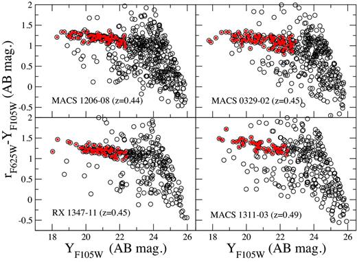
An example composite colour–magnitude diagram for the CLASH fields containing clusters in the 0.44 < z < 0.49 interval, identified in the figure legends. Photometric errors on colour measurements of individual red sequence galaxies vary from <0.01 at Y = 19 to <0.05 at Y = 23. The symbols in this diagram represent all galaxies detected in these fields (irrespective of cluster membership). The prominent red sequence in each diagram is formed by passively evolving galaxies in each target cluster. Solid red symbols identify the CRSGs analysed to determine their structural parameters. See Supplementary Information for other clusters in CLASH and Paper I for the very high redshift sample at z > 1.
We select galaxies within ±0.25 mag of the mean colour–magnitude relation for the red sequence, as determined by fitting a straight line to the data by linear minimum absolute deviation (Beers, Flynn & Gebhardt 1990). In the absence of extensive spectroscopic information, the red sequence selects a sample of cluster members with comparatively minimal contamination by galaxies in the foreground and background (cf. Rozo et al. 2015). While this means that some contamination may be present, to the limits of our analysis its effect is not overly significant. For example, Fig. 1 shows that to Y ∼ 23 (more than 1 mag fainter than our typical analysis limit) the red sequence of a subset of z ∼ 0.45 clusters appears to be well separated from other objects: similar conclusions can be drawn for other clusters (e.g. see the equivalent figure in Paper I). In this and equivalent figures, the galaxies we have eventually studied (for structural analysis) are marked as red dots; a few objects in each cluster (even if they were on the red sequence) could not be modelled or the residuals seemed to indicate a poor fit. As these represent only a small fraction of our sample, we have not considered them further.
The red sequence has been commonly used as an indicator of cluster membership, at least for the dominant quiescent population of (typically) E/S0 galaxies. As a test of this method, two of our clusters have extensive public redshifts from the CLASH-Very Large Telescope (VLT) survey. In MACS 1206, 62 of our 100 galaxies on the red sequence have a redshift measured from Biviano et al. (2013) and Rosati et al. (in preparation). Of these 61 are cluster members. In MACS 0416, 122 of the 158 galaxies we study on the red sequence also have a redshift from Balestra et al. (2016) and of these 118 are cluster members. Therefore, our method selects cluster members with a fidelity exceeding 95 per cent. Of course higher redshift clusters, and fainter galaxies in any clusters, may suffer from somewhat higher contamination, as we have discussed in Paper I. Since the redshift completeness, even for the clusters in CLASH-VLT, is no greater than 60 per cent, and not all CLASH clusters are observable from VLT, we still need to use red sequences to select a sample of cluster members in all our clusters.
By construction, our red bands are chosen to match the rest-frame R band, with a small colour term (e.g. as in the example above in Fig. 2, the central wavelength of the adopted filter is only 5 per cent different from the actual R band). This colour term is however difficult to calculate accurately, as it depends sensitively on the spectral energy distributions of galaxies and their evolution. In order to be able to compare the luminosity distributions at different redshifts, we corrected all magnitudes to the rest frame R at z = 0.22 (the mean redshift of the five closest CLASH clusters) to provide a reference magnitude, denoted as Rz = 0.22. We assume a passively evolving model from Bruzual & Charlot (2003) with zformation = 3, solar metallicity and an e-folding time of 1 Gyr. Previous work has shown that this model yields a good fit to the observed colours of CRSGs across a wide range of redshifts (Mei et al. 2012).
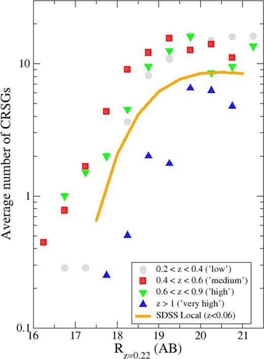
The averaged luminosity distributions of galaxies on the red sequences of CLASH clusters (14 clusters for the low-redshift sample, nine for the medium-redshift and two for the high-redshift group), shifted to z = 0.22 (assuming a passively evolving model as described in the text), and our z > 1 sample (of four clusters) in Paper I (symbols as identified in the legend) compared to the local cluster SDSS r-band red sequence luminosity function as derived by Rudnick et al. (2009), with arbitrary normalization to best show the match in shape.
We group the CLASH clusters into three subsamples: (i) 14 clusters at 0.19 < z < 0.40, the ‘low’ subsample; (ii) nine at 0.44 < z < 0.58, the ‘mid’ subsample; (iii) two at z = 0.69 and 0.89, the ‘high’ sample and combine these with the ‘very high’ 1 < z < 1.4 sample from Paper I (see Table 1). The relatively small size of the ‘high’ sample is due to the paucity of systems observed in the appropriate bands with HST (ACS F814W and WFC3 F125W or F160W). The number of CRSGs in each subsample (identified via the red sequence) is 1037 for ‘low’, 743 for ‘mid’, 136 for ‘high’ and 87 galaxies for ‘very high’ (Paper I) to Rz = 0.22 = 21.
2.3 An R-band limited sample of galaxies
We select galaxies on the red sequence of each cluster and calculate the average number of objects in each of the ‘low’, ‘medium’, ‘high’ and ‘very high’ redshift subsamples, within 0.5 mag bins in Rz = 0.22 down to a magnitude where we believe contamination to be minimal and red sequences are well isolated in the surrounding colour space (see Fig. 1).
We plot the average counts (i.e. divided by the number of clusters in each subsample) in Fig. 2 versus Rz = 0.22, omitting the error bars to avoid confusion (but the errors are Poissonian, since these are simple counts and do not include the clustering contributions from the field). This may be considered as a luminosity distribution rather than a luminosity function as we have not removed possible contamination from fore/background objects (all clusters are studied in different observed bands, not all of which have sufficiently deep, or even any, observations of comparison fields). For comparison, we plot the z = 0.06 r-band luminosity function of cluster red sequence galaxies (corrected to our bandpass and redshift) from the SDSS (Rudnick et al. 2009). The normalization is chosen arbitrarily to best show the differences in the shapes of the red sequence luminosity distribution across the redshift ranges we study and to provide a local comparison (this normalization is usually left to float as it does not have a clear physical meaning for clusters).
The average composite luminosity distributions for the CRSGs drawn from the ‘low’, ‘mid’ and ‘high’ subsamples are consistent with the passively evolved Schechter functions for local and ‘very high’ redshift clusters having |$R^{\ast }_{z=0.22} \sim 19.1$| (the characteristic magnitude M* measured in the R band shifted to z = 0.22 as described above) and α ∼ −1. The mean number of galaxies in the CLASH sample in each magnitude bin is also comparable, suggesting that we are typically observing objects of comparable environmental density. The number counts of galaxies in the high-redshift sample of Paper I are also broadly consistent with those measured for CLASH clusters, suggesting that we are not observing objects with very different properties across the redshift range of interest.
Given this selection, brighter than an evolved Rz = 0.22 of about 21 (approximately MR = −18, or down to about 1/5th the luminosity of the Milky Way) we are studying objects that have broadly the same stellar mass and passively evolving stellar populations at all times out to z ∼ 1.25. The good match to the local luminosity function of Rudnick et al. (2009) and to the results of Paper I confirms the essentially passive evolution of red sequence galaxies in CLASH clusters. While these results are already well known, their recovery confirms that our selection of the photometrically defined red sequence galaxies as cluster members is appropriate for the purposes of this study. Therefore, our sample consists of similar galaxies at all redshifts, linked by the observed passive evolution on the red sequence. To Rz = 0.22 ∼ 21 we have a complete sample where we study galaxies of similar luminosity and colour at all redshifts with relatively little contamination from non-cluster sources.
3 STRUCTURAL PARAMETER EVOLUTION
We determine structural parameters for the CRSGs in the rest-frame B and R using galfit (Peng et al. 2002, 2010) as in our previous analysis of z ∼ 1.25 clusters in Paper I.
For each galaxy we carry out an interactive and iterative process, where we adopt reasonable starting values and proceed to inspect the model and residuals to ascertain the quality of the fit (i.e. we do not run galfit in batch mode, but individually for each object). Where necessary, multiple models are run together, e.g. in the case of close pairs or systems of galaxies. We adopt a single Sérsic profile. This is warranted by the relatively shallow CLASH data and can also be more easily compared to previous work in cluster and field galaxies. For each image and in each band we use the median of several bright, unsaturated and isolated (as possible) stars to derive a point spread function (PSF) reference, with min/max clipping of eventual interlopers in the chosen field. Typical PSF image sizes are 100 times the full width at half-maximum (FWHM) of the PSF (as recommended by the galfit manuals). This procedures ensures that the PSF incorporates all processing steps to which the images of the galaxies have been subjected and is therefore preferable to generating artificial PSFs (e.g. with TinyTim). For each galaxy being considered the sky level is determined locally within the large aperture needed for analysis by galfit (including assessment of eventual gradients by fitting a surface to the sky – see below). The results of this procedure are the effective radii (in rest-frame B and R), the Sérsic indices (also in both bands) and the axial ratio b/a (also in B and R rest frame). From these we derive the colour gradient Δ(B − R)/Δlog r, following the formula given in La Barbera et al. (2002, 2003) using the measured structural parameters in each band.
Particularly for the higher redshift samples, the pixel scale of the images (0.03–0.08 arcsec) is a significant fraction of the effective radius (at z = 1, 1 arcsec corresponds to 8 kpc, with typical galaxies having Reff of 1 kpc, e.g. Gutiérrez et al. 2004) and the PSF FWHM has a size comparable to the effective radius (0.05–0.08 arcsec depending on the bandpass and instrument used). Any 2D profile, e.g. produced with the irafellipse package (Jedrzejewski 1987), will be heavily affected by sampling and by the PSF size. Furthermore, mismatches in the galaxy centroids and the different PSFs in the red and blue bands (often using two different instruments: ACS in the optical and WFC3 in the infrared) will result in spurious colour gradients (e.g. La Barbera et al. 2003). Using fits to structural parameters from galfit modelling of the full image, automatically removes these sources of error. We therefore use our derived parameters in the subsequent analysis rather than attempting more detailed profiling.
It is known that the errors output by galfit can sometimes be significant underestimates in the case of small images. However from the work of Haussler et al. (2007) who simulated HST images very similar to those used here, in terms of magnitude, surface brightness and size, it can be seen that galfit will provide values of Reff accurate to within 5 per cent down to magnitude 22.5, even for steep (n ∼ 4) profiles. Errors in n are ∼0.25 at n ∼ 4 and much less at n ∼ 1, while ellipticity errors are typically 0.04. Errors of this size, for the faintest objects we analyse, are sufficiently small that they do not influence any of our results.
In addition, we have run a series of simple simulations of our own with irafartdata to test our procedures. These introduce idealized galaxies (pure exponentials or pure spheroids obeying the deVaucouleurs law) in ‘clean’ regions of the images. Using galfit on the simulated images confirmed that parameter errors were of the level noted above or smaller (the dispersion in values was consistent with the errors returned by galfit, i.e. within 1 per cent) and that galfit parameters could be used safely down to the faint limit of our analysed data.
We have further introduced artificial sky gradients to simulate the effects of intracluster light and galfit is found to be insensitive to any such smooth gradients, unless they vary rapidly across the galaxies over scales comparable to the effective radius; even then, the result is not incorrect parameters but catastrophic failures of the iteration. When this does not happen, the errors returned are consistent with the galfit output, i.e. ∼1–2 per cent. Since we actually inspect each object (model and residuals) individually, we can rule out the presence of such pathological sky features at any levels that would interfere with the fitting procedure.
4 RESULTS
4.1 Size evolution
Fig. 3 shows the size distribution versus R-band magnitude (shifted to z = 0.22 assuming the concordance cosmology and a passively evolving model as described above) for all galaxies in the CLASH cluster sample and the sample from Paper I. The appearance of the distribution is similar to that found in local systems (e.g. Coma in Gutiérrez et al. 2004), with a cloud of systems at intermediate sizes of 1–2 kpc and a brighter sequence of large, luminous galaxies; these latter objects tend to be high n early-type spheroid-dominated galaxies (classical E/S0). We compare the size distributions of galaxies brighter than Rz = 0.22 = 21 in the right-hand panel of Fig. 3 (including the z > 1 sample in Paper I).
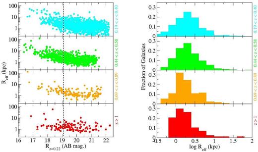
Left: size distribution for galaxies in clusters. We plot the effective radii from single Sérsic profiles versus the R magnitude at z = 0.22 (where this is actually the HST band closest to rest-frame R, accounting for passive evolution and cosmology) for groups of clusters at ‘low’ (0.19 < z < 0.40), ‘mid’ (0.44 < z < 0.58) and ‘high’ (0.69 < z < 0.89) redshifts in the CLASH sample. We also plot the z > 1 (‘very high’) results from Paper I in the bottom panel (as indicated in the figure). The errors returned by galfit on these parameters are typically below 1 per cent and smaller than the size of the points. The grey line shows the M* value derived by Rudnick et al. (2009) for local clusters in the R band, corrected to z = 0.22 with the concordance cosmology and the passive evolution model (i.e. |$R^{\ast }_{z=0.22}$|). Right: size distribution for galaxies in clusters at all redshifts we consider. Each panel corresponds to a redshift interval as indicated in the legend. The bottom panel shows the data from Paper I for the ‘very high’ (z > 1) sample.
In order to take into account both the shape and absolute numbers of objects contributing to each distribution in Fig. 3, each was compared to the others using a standard Kolmogorov–Smirnov (KS) test. The ‘very high’ distribution differed from the ‘low’ and ‘middle’ at the 3σ and 2σ levels (P = 0.02 and 0.06), respectively (assuming a Gaussian distribution), i.e. unlikely to be drawn from the same distribution. Similarly, the ‘high’ distribution differed from the ‘low’ and ‘mid’ distributions at the ∼3σ (P = 0.02 and 0.04) levels, respectively. Below z ∼ 0.6 there appears to be no significant size evolution, while for higher redshifts, we can characterize the change by the typical Reff decreasing by at most a factor ∼1.5 over 0.7 < z < 1.4 given that the peak of the size histogram shifts by at most one bin (0.2 dex) in Fig. 3. The large sizes of some of our brightest cluster galaxies are also consistent with the findings of Stott et al. (2011) and Lidman et al. (2012). Stott et al. (2011) use both a method very similar to ours (with galfit) and also the irafellipse package from sdsdas, finding very similar results, suggesting that the measured sizes are insensitive to the precise modelling technique (Stott, private communication).
The results shown in Fig. 3 are broadly consistent with the form of size evolution identified by Delaye et al. (2014) from ground-based near-infrared (IR) imaging, through a comparison between systems at 0.8 < z < 1.5 and z = 0 (Reff ∝ (1 + z)−0.5) with most, if not all of the evolution, taking place well above z ∼ 0.6 and probably beyond z ∼ 1. Any size evolution in CRSGs in the past ∼9 Gyr appears to be much smaller than that found in field samples of quiescent galaxies of comparable luminosity over the same redshift range (Cerulo et al. 2014; Delaye et al. 2014; Saracco et al. 2014; Paper I). Kelkar et al. (2015) observe that at 0.4 < z < 0.8 early-type galaxies have roughly the same size as local ones, in agreement with our findings for the ‘low’, ‘mid’ and ‘high’ subsamples. Newman et al. (2014) detects no more than a 30 per cent change in the size of red sequence galaxies with stellar masses higher than 109.8 M⊙ between z = 0 and 1.8 (also see a forthcoming paper by Andreon, private communication).
van der Wel et al. (2014) and Huertas-Company et al. (2015), among others, however find that the average field early-type galaxy increases its Reff by a factor of 3 or more, mainly since z ∼ 1.5, with growth continuing all the way to z = 0, unlike this cluster sample. The degree of size evolution appears to depend on environment: Lani et al. (2013) and Damjanov et al. (2015) also find evidence that size evolution is weaker in high-density environments (by as much as 50 per cent in Lani et al. 2013 when looking at their densest systems). However, note that our clusters are considerably more massive than any of the objects studied by Lani et al. (2013) or Damjanov et al. (2015). Given the already known passive evolution in colour and luminosity, the small change in size observed for these galaxies appears to suggest early formation and assembly, with little subsequent evolution, especially by mergers, and most other changes being due to internal processes or more gentle external inputs, a conclusion also reached by Huertas-Company et al. (2015) at least for the more massive spheroidals in the field.
4.2 Sérsic index evolution
As in the previous subsection, we now plot the evolution of rest-frame R-band Sérsic indices (n) as a function of redshift for CRSGs in Fig. 4. The corresponding histograms for the distribution of n values is shown in the right-hand panel of Fig. 4, including the 1 < z < 1.4 data in Paper I.
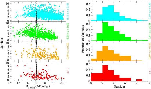
Left: distribution of Sérsic indices for galaxies in clusters. We plot the Sérsic index n versus the R magnitude at z = 0.22 as in the previous Fig. 3, for groups of clusters at ‘low’ (0.19 < z < 0.40), ‘mid’ (0.44 < z < 0.58) and ‘high’ (0.69 < z < 0.89) redshift in the CLASH sample. We also plot the z > 1 results from Paper I (‘very high’) in the bottom panel. Errors returned by galfit are smaller than the size of the points (typically <0.01 in n). Right: Sérsic index distribution for galaxies in clusters as in the previous Fig. 3 and indicated in the legend. There is evidence for an increasing presence of disc-like components among red sequence cluster galaxies as a function of lookback time.
At low redshift (z < 0.6), clusters are dominated by a population of spheroidal galaxies, with n > 2.5 corresponding to classical E/S0 galaxies as expected, with very few objects with n < 2. However, at higher redshifts an increasing fraction of the population have low Sérsic indices consistent with the presence of disc-like components (Fig. 4). Whereas for z < 0.6 about 30 per cent of galaxies are observed to have n < 2.5 and the median n is ∼3.3, this fraction rises slightly (to about 35 per cent) in the 0.6 < z < 0.9 sample and in the highest redshift subsample more than 50 per cent of galaxies have n < 2.5 and the median n is 2.2, with only brighter cluster members tending to be n > 4 spheroids.
Again, KS tests were carried out between each of the subsamples. The Sérsic index distribution of the ‘very high’ subsample differed from each of those of the other three subsamples at more than the 5σ level (P < 0.01). The ‘high’ and ‘mid’ distributions showed no convincing differences from each other, but both differed from that of the ‘low’ subsample at the approximately 2σ (P = 0.04) level, implying ongoing evolution towards the low-redshift distribution to about z ∼ 0.5–0.6. Looking at Fig. 4 any evolution below z ∼ 1 is likely to be more subtle than that at higher redshifts and may only require evolution in a subset of the galaxies to achieve the observed differences.
Inspection of the B-band images confirms this impression. In Paper I (see fig. 7) we saw that most n < 2 galaxies have significant disc-like components, even though they lie on the red sequence. In this paper, we plot similar postage stamps of all such galaxies in CL 1226+3332 (z = 0.89), the highest redshift cluster in the CLASH sample, in Fig. 5, showing that disc-like objects start to become significant at this redshift, including some slightly clumpy systems. Both Rembold & Pastoriza (2012) and Cerulo et al. (2014) also observe numerous faint disc-like galaxies in two z = 1 clusters.
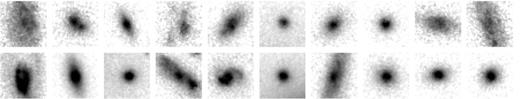
HST/ACS 2 × 2 arcsec2I-band images for 20 red sequence galaxies with n < 2 and magnitudes within ∼1 mag of |$M^{\ast }_R$| from the z = 0.9 cluster CL 1226+3332. Presentation is the same as that for fig. 7 in Paper 1 with the grey-scale stretching between the mean sky level to the square-root of the central surface brightness (so more diffuse, lower surface brightness galaxies appear to have noisier images).
This reinforces our previous finding: red sequence galaxies in high-redshift clusters appear to contain an increasingly important disc-like component at higher lookback times. While local S0 galaxies certainly have discs, their overall Sérsic indices are still typically n ≥ 2.5. Consequently this disc-like component at high redshift must eventually either disappear or evolve by z ∼ 0.6 where the population closely resembles that of present-day clusters. The end-state of these high-redshift CRSGs (with significant discs) must be the S0 and elliptical galaxies that dominate at higher n and lower redshifts. In some respects, this finding resembles the observations by Buitrago et al. (2013) in the general field, where apparently quiescent galaxies exhibited an increasing contribution from disc-like systems at z > 1. Similarly, Huertas-Company et al. (2015) observe bright n ≥ 4 spheroids formed at high redshift, and an increasing proportion of irregular and thin discs at lower luminosities and higher redshifts. In order to ascertain the nature of the disc-like components we next look at the shape of the objects via their axial ratios.
Below z ∼ 0.6 our clusters contain mainly, if not solely, galaxies with effective radii, Sérsic indices and axial ratios (see below) consistent with z = 0 systems. Such objects likely resemble conventional E/S0 galaxies (to the extent that such classification is objective and appropriate, considering the nature of the data). We do not carry out a study of such classifications here, as we are interested in the change in structural parameters and quantifiable measures of evolution.
4.3 Axial ratio evolution
In Fig. 6 we plot the distribution of b/a (axial ratios) versus Rz = 0.22 magnitude for all our clusters in the same fashion as for sizes (Fig. 3) and Sérsic indices (Fig. 4). We also plot the corresponding axial ratio distributions in Fig. 6.
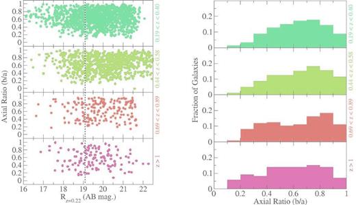
Distribution of axial ratios for galaxies in clusters in the previously defined subsamples. Errors on axial ratios returned by galfit are smaller than the size of the points Right: axial ratio distribution for galaxies in clusters as in Fig. 4 (see legend). There is evidence for an increasing disc fraction (oblateness) among a subset of the CRSGs as a function of lookback time.
At z < 0.6 the axial ratio distributions indicate a population dominated by objects with low apparent ellipticity, either true ellipticals or systems with comparatively thick discs such as S0s. The distribution peaks close to the local (z = 0) values in Ryden, Forbes & Terlevich (2001), i.e. b/a ∼ 0.7–0.8. The axial ratio distributions of the two higher redshift populations instead appear by eye to be flatter, with a significantly higher proportion of systems with projected axial ratios reaching down to ∼0.2. Such distributions are unlike those achievable through a mixture of ellipticals and typical S0 galaxies (Lambas, Maddox & Loveday 1992) and again indicate an additional population with significant disc-like components at z > 0.6 with an axial ratio distribution closer to that of field spirals (Graham & Worley 2008): the mean axial ratio in the highest redshift bin is 0.58, closer to that observed in spiral discs (Ryden 2004). KS tests indicate significant differences between the ‘very high’ and both the ‘mid’ and ‘low’ subsamples at about the 2σ levels (P = 0.05 and 0.09, respectively), but no other significant difference.
Buitrago et al. (2013) also find some evidence for increasing flattening with redshift, implying a more prominent role for disc-like components in galaxies, while Chang et al. (2013) find an increase in the fraction of oblate objects at z > 1. However, unlike their results we have an increasing fraction of flatter galaxies at the lower luminosity end in the higher redshift bins. Papovich et al. (2012) already noted the presence of elongated galaxies on the red sequence for a z = 1.62 cluster, while Holden et al. (2009) have found no change in the shape of cluster galaxies selected as S0 with redshift, which implies that our flattened ‘discs’ might eventually thicken and become rounder, in order to join the population of present-day S0s.
4.4 Colour gradients evolution
A further clue to the evolution of galaxies may be provided by radial colour gradients. These reflect the 2D distribution of stellar populations as well as their kinematics. The existence of colour gradients in nearby ellipticals (e.g. Saglia et al. 2000; Tamura & Ohta 2000) is best explained as being due to a mild metal abundance gradient with radius (richer inward) and its apparent dependence on galaxy luminosity (e.g. in Coma; den Brok et al. 2011) suggests a model where the majority of the stellar populations were assembled early in rapid mergers or dissipational collapses, as a more extended hierarchical merger scenario would tend to erase such gradients (Kobayashi 2004).
In Paper I we showed through the ratio of rest-frame B- and R-band Reff that the 1 < z < 1.4 CRSGs had significant radial colour gradients, becoming bluer with radius. The strength of these gradients was such that they could not be explained by abundance variation, implying that they were a symptom of radial age gradients in the stellar population of each galaxy. Following Paper I, we have derived colour gradients for our galaxies, extending the treatment by converting the observed Reff and n in the two B and R bands to a more conventional Δ(B − R)/Δlog r (La Barbera et al. 2002). To do this we determine the colours at 1 and 2Reff, sufficiently large radii to not have the measurement compromised by either the PSF or pixel size, even for the most distant objects.
In order to display the results of this procedure and gain insight into how the gradients depend on stellar mass, for each redshift range we show the derived colour gradients and best-fitting straight line from a biweight estimator (e.g. Beers et al. 1990) in Fig. 7, plotted versus Rz = 0.22 as in previous figures. The units of the colour gradients are magnitudes per decade in radius. The statistical uncertainty on each derived value is low (typically <0.1 mag per decade in radius) given the errors on n and Reff from galfit (typically less than 1 per cent). Consequently the scatter in and breadth of the distributions is a real reflection of the scatter in the properties of the objects at each redshift.
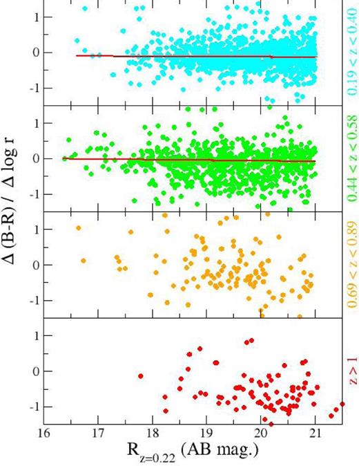
Colour gradients for galaxies in clusters at all redshifts we consider. Each panel corresponds to a redshift interval as indicated in the legend.
At lower redshifts, the mean values of the colour gradient at each R-band magnitude are consistent with the usual mild colour gradients (about 0.1–0.2 mag blueward per decade in radius) seen in nearby clusters. At these redshifts we also confirm the existence of a mild trend with luminosity (and presumably stellar mass) extending over 3–4 mag, in the sense that fainter galaxies have milder colour gradients, as seen in the Coma Cluster (den Brok et al. 2011). This relationship appears to persist at least out to z ∼ 0.6 in agreement with earlier studies by La Barbera et al. (2003). Linear fits (with minimum absolute deviation) to the data are shown for the ‘low’ and ‘mid’ redshift bins in Fig. 7. If we interpret the observed gradients as metal abundance gradients, then our data are consistent with a trend of metal abundance with stellar mass, in the sense of galaxies with steeper potential wells having more significant gradients, as in Coma (den Brok et al. 2011). This is more consistent with an inner region dominated by old stellar populations formed dissipationally at high redshift, either by gas-rich early mergers or large-scale gaseous collapses (e.g. Oser et al. 2010).
The picture changes at higher redshifts. At z ∼ 0.2 the gradient is typically −0.1 mag at Rz = 0.22 = 20 while at z > 0.6 this becomes −0.5 mag, but with a larger scatter. At z > 0.6 the outskirts of galaxies seem to become increasingly blue relative to their centres and show an increasing object-to-object scatter in the strength of the gradient (cf. Paper I; Chan et al. 2016 for a similar result). For this reason we do not carry out fits to the data in the ‘high’ and ‘very high’ bins in Fig. 7. The appearance of comparatively strong colour gradients at z > 0.6 is consistent with the results at z ∼ 1.25 in Paper I where the outskirts of the CRSGs were clearly bluer than their centres (even though they were globally red in colour by selection). At these redshifts a significant minority of sources with Rz = 0.22 > 19 appear to have gradients with strength more easily achievable through stellar age gradients, rather than variations in metallicity as is common at lower redshifts.
In order to explore how the variation in the strengths of colour gradients maps on to potential differences in both age and metallicity of stellar populations in bulge and disc components, we generated the luminosity and colour evolution with redshift for two possible components of the galaxies using Bruzual & Charlot (2003) SSP models. We assumed a component that formed in a single burst at z = 3 with solar metallicity and determined its variation in rest-frame B − R colour and mass to light ratio at z < 1.5. This can be taken to be representative of a maximally old bulge component (or indeed a similarly old disc component). For purposes of this exercise we assume that this represents a maximally red model for the central regions of one of our galaxies. We then did the same for a component undergoing a similar burst at z = 1.5 with either solar or 0.25 solar metallicity. The lateness of this burst was chosen simply to give the maximally blue colour and most rapid colour evolution below z = 1.4 rather than attempting to mimic any individual galaxy. In effect, it places an upper bound on the variation in colour that can be attributed to variations in population age and metallicity across a galaxy.
The range of colour differences between the old and younger stellar populations, and its evolution with redshift demonstrates that the variation and evolution in colour gradients observed in the population of CRSGs can be potentially explained through a combination of metallicity and age-related gradients. The age-induced gradients decrease with time as both populations converge towards similar colours ∼5 Gyr after the most recent burst, revealing the underlying gradient due to the (known) radial metallicity gradients (see also Chan et al. 2016 for a similar conclusion). While similar colours may in principle be achievable if the younger component included some ongoing star formation below z = 1.4, this behaviour is constrained by the lack of evidence for such activity in cluster red sequences below this redshift. The differential colours shown in Fig. 8 are for two components of equal stellar mass. Given that specific star formation rates in these galaxies are usually well below 10−10 yr−1, it is difficult to see how the colour gradients observed at z > 0.6 are achievable through ongoing star formation alone.
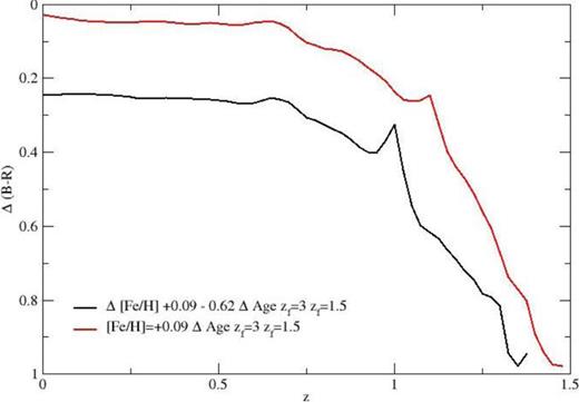
Difference in colour between a solar metallicity SSP burst at z = 3 and two SSP bursts at z = 1.5 when viewed at z < 1.4. The two younger SSPs have metallicities of approximately 0.25 and 1 times solar. These models illustrate the most extreme colour differences likely to occur in a quenched system with two different stellar populations. The oldest burst represents a bulge population and the youngest a disc. In reality both are likely to consist of stars from more extended periods of star formation, decreasing colour differences between them relative to those derived here. Nevertheless, the models demonstrate that the colour gradients observed in the CRSGs studied here can plausibly be explained by a mix of age and metallicity related gradients, with the age-induced gradients dominating at earlier times over the metallicity gradients.
A similar argument is presented by Chan et al. (2016) who analyse one of the clusters we studied in Paper I and reach consistent conclusions to ours: the presence of an age gradient superposed over a more ancient weak metallicity gradient, although they do not make the explicit connection to the presence of disc-like components. Studying red discs in the SDSS Lopes et al. (2016) also argue for a quenching time-scale of around 2–3 Gyr (in agreement with our work and Chan et al. 2016) and the gradual morphological evolution of the red discs as they move towards cluster centres.
5 DISCUSSION
Paper I explored the morphological differences between a sample of z > 1 CRSGs and their nearby counterparts. A significant fraction of the reasonably bright ( ∼ L*) high-redshift systems had structural parameters that were consistent with more disc-like morphologies than those of their low-redshift counterparts. The brightest galaxies in the red sequence appeared to be different, in that their morphological parameters were already closer to local early-type ellipticals, indicating any structural evolution was completed at earlier epochs for this brighter subsample. What was not established in Paper I was the time-scale over which any morphological transformation occurred in the more typical red sequence galaxies. The results within this paper help to determine this time-scale by exploring the same structural parameters for CRSGs drawn from clusters observed at several intervening epochs.
A key result of this work appears to be that for most of the structural parameters in question, any strong evolution has largely been completed by z ∼ 0.5–0.6, a lookback time of 5–6 Gyr, and 3–4 Gyr after the latest redshift (z ∼ 1.4) that any star formation in the red sequence galaxies is likely to have been quenched (e.g. Tran et al. 2010). At higher redshifts there is good evidence (albeit limited by the number of systems with useful HST data at 0.6 < z < 1) that the relevant parameters are transitioning between the local distributions and those found in Paper I. As the velocity dispersions are already very high in these massive clusters and the luminosity function evolution disfavours significant major merging, this process must take place secularly or by more gentle external inputs (such as minor mergers or fly-bys).
All of this data is consistent with a simple picture outlined in Paper I where, after quenching, ∼ L* red sequence galaxies do not evolve in colour and luminosity other than the passive evolution of their stellar populations, but a proportion undergo considerable morphological change over the past 2/3 of the Hubble time. The brightest and more massive cluster spheroids in this sample seem to have already arrived at their final configuration by the beginning of this period (cf. Saracco et al. 2014) but fainter galaxies are likely to show significant evolution, analogous to the observations by Huertas-Company et al. (2015) in the CANDELS field. However, most of our discussion as to the former must be qualitative for now, as there are too few bright galaxies in the small number of high-redshift clusters that we observe to draw statistically valid conclusions.
Within this picture, the CRSG population as a whole appears to become slightly less compact with time, although the scale of this growth is significantly less than that seen for passively evolving field galaxies of similar mass over the same time period. The evolution is reminiscent of that observed in previous studies (Delaye et al. 2014), although it may be even weaker, compared to the field, because of the much higher environmental density (if the trends observed by Lani et al. 2013 can be extended to clusters). At the same time CRSGs also become less disc dominated with decreasing redshift. The decreasing importance of the disc component is reflected in changes to all of the structural parameters, including the Sérsic index n and the axial ratios. Similarly to Buitrago et al. (2013) and Chang et al. (2013) we observe an increasing contribution from disc-like components at z > 1 and somewhat more oblate galaxies, with axial ratios closer to those of spiral discs (cf. Rembold & Pastoriza 2012; Cerulo et al. 2014).
The brighter and more massive galaxies may constitute a class apart. Brightest cluster galaxies, for instance, are often believed to follow a more distinct evolutionary history than the less massive cluster population. We show the actual data in Figs 3, 5 and 7 for all objects. However, if we consider only the 10 per cent brighter (and likely more massive) systems, the values for Reff and n are consistent with no significant evolution (i.e. these bright ellipticals appear to have reached their ‘final’ status early on in the history of the Universe) but the statistical power afforded by the small number of objects in the highest redshift samples does not suffice to draw strong conclusions on the evolution of these objects.
5.1 A strawman model for morphological evolution
Here we summarize a strawman model for this evolution which can explain the results described above, and poses further useful questions on the details of this evolution. This model contains elements that will be familiar to anyone with a knowledge of the early studies of galaxy evolution (e.g. Larson, Tinsley & Caldwell 1980). The model need not apply to each individual galaxy on the red sequence, rather it describes the evolution necessary within a subset of CRSGs in order to produce the changes in the distributions of structural parameters over time.
At high redshift (z > 1) we begin with a significant fraction of CRSGs having disc-like components that are both thin and have younger and more metal poor (bluer) stellar populations than their central spheroids. We associate the disc component with recently quenched star formation seen at z > 1.5 (e.g. Tran et al. 2010), so while it is bluer than the spheroid component, it is in the first stage of passive evolution and its photometric properties evolve rapidly. The model assumes a metallicity gradient (e.g. as for local samples of early-type galaxies; Rawle et al. 2010; Kim & Im 2013) between the two morphological components, consistent with the many observations of radial metallicity gradients in disc galaxies (e.g. Moustakas et al. 2010, and references therein). In local discs, one observes metal abundance gradients of −0.2 to −0.6 dex per decade in radius (from the direct method of line ratios in planetary nebulae and H ii regions within resolved discs, as in Moustakas et al. 2010), which would yield colour gradients (from Fig. 8) of the magnitude observed in local samples (such as the brighter members in Coma from den Brok et al. 2011). The effect of the metallicity difference on radial colour gradients is only evident at lower redshift as the difference in age of the bulge and disc components dominates at higher redshift.
Given the constraint imposed on the overall colours of the galaxies by red sequence selection, the fraction of the mass provided by any disc must be severely constrained, even when there is a colour gradient. Fig. 8 shows the colour difference between two equal mass SSP bursts with different formation times. Given the width of the rest-frame B − R red sequence is only a few tenths of a magnitude and includes objects with a range of Sérsic indices at all redshifts studied here, it is likely that any young disc component carries no more than ∼10 per cent of the total stellar mass in a typical CSRG. Obviously any extended period of star formation in such a disc has less effect on the overall colour and therefore can contain more of the mass. Cen (2014) shows how spiral galaxies evolve almost vertically in colour space and rapidly on to the red sequence once their star formation is terminated, in agreement with the scenario presented here, where such objects are present on the red sequence but still preserve their ‘spiral’ morphologies, with thin discs.
With increasing time since quenching the disc fades and reddens faster than the older spheroidal population. After 3–4 Gyr the difference in colours between the two components is largely dominated by the different metallicities and both fade and redden at approximately the same rate (as in Fig. 8). This leads to the decreasing magnitude of and scatter in colour gradient with time. Over time the disc should also thicken to explain the changing axial ratio distribution for the population. This could simply be caused by the quenched thin disc fading to reveal an underlying thick disc, or other internal and external processes could continually act to thicken the disc. The precise mechanisms are beyond the scope of this paper and there may be several processes contributing to this, such as disc instabilities or the addition of structure in the outskirts. However, simulations by Gnedin (2003a,b) demonstrated that the continual tidal heating suffered by disc galaxies subsequent to their infall into clusters was sufficient to thicken their discs by a factor of ∼2 over their lifetime in the cluster, effectively transforming the shapes of late-type spirals into those of S0s (Laurikainen et al. 2010). Over the same time, and for the same reason, the Sérsic indices of those systems with the (initially) most prominent discs change from n < 2 to values more consistent with S0 galaxies, 2 < n < 3, straightforwardly explaining the evolution seen in Fig. 4. A clear implication of this model is that we can link the high-redshift CRSGs with relatively blue and thin discs to the S0 galaxies with small colour gradients and thicker discs seen to populate cluster red sequences at intermediate and low redshifts at ∼ L* and below. As the shapes of galaxies selected morphologically as E/S0 by Holden et al. (2009) do not change over time, our disc-like red sequence galaxies must naturally evolve to resemble present-day E/S0s.
A key recent work on the low-redshift cluster S0 population is that of Head et al. (2014), exploring the parameters of this population in the Coma Cluster. The simple model outlined here produces galaxies with photometric properties consistent with those determined by Head et al. (2014). Note that because S0 galaxies exist on the red sequences of clusters at all redshifts, the model does not imply that all low-redshift cluster S0s formed in this manner in the range 0.6 < z < 1.4, merely that the S0 population was significantly augmented over this time.
5.2 Limitations of the model and the current data
There are several significant issues that are not constrained by this simple model and the existing data. The first is the reason for the quenching of star formation in disc components. This could simply be attributed to a loss of fuel after infall into the cluster. As ever, suspects for such clustercentric mechanisms include ram pressure stripping (e.g. Tonnesen & Bryan 2009; Cen 2014), virial shock heating (Birnboim & Dekel 2003) and strangulation (e.g. Larson, Tinsley & Caldwell 1980; Peng, Maiolino & Cochrane 2015) amongst others. Alternatively, it could be due to a secular process, such as morphological quenching (Martig et al. 2009; Huertas-Company et al. 2015), where the spheroidal component of a galaxy grows to a size sufficient to stabilize the disc against further star formation. As long as star formation in any disc is ended by z ∼ 1.5, any of these mechanisms may result in the systems at 1 < z < 1.4 identified in Paper I having disc-like components.
A second issue is that of bulge growth. Although the model above was framed in terms of disc fading, because we are measuring the evolution in relative strength of bulge and disc components with time there could equally be a role for bulge growth in this evolution. Work has recently been presented on the maturity of bulges and the quenching of star formation in z ∼ 2 star-forming galaxies drawn from a range of environments (Tacchella et al. 2015). This indicated that these systems quench star formation from the inside out and that their central (bulge) surface densities are already comparable to those of similar stellar mass z = 0 early-type galaxies with stellar masses above 1010M⊙, and within a factor of 2 of the z = 0 values even for lower mass systems. The implication is that barring any subsequent mass growth through mergers, the bulges of galaxies with similar masses to those explored here are already largely in place by z ∼ 2. The CRSGs explored in Paper I and here either originated in the field and subsequently fell in to their clusters, or formed in an accelerated manner in existing high-density regions as part of the original growth of the hosting clusters; it might be expected that their central spheroidal components are already in place before any disc component starts to quench. Given the already-noted limit to how much mass can be in any relatively young stellar disc given the narrow colour range in cluster red sequences, coupled with the lack of growth of total stellar mass in the same galaxies since z ∼ 1.4 (Paper I), it would seem that the bulges would have to be in place by z ∼ 1.4. However, that does not account for any older disc component which could evolve morphologically, growing the bulge through inflow of stars and other material over time.
In order to test this we determine the luminosity in the R band within the central 1 kpc (Σ1) for each galaxy by integrating its fitted Sérsic profile out to this point. This may be thought of as a proxy for the central density (as used by e.g. Fang et al. 2013 in their study of low-redshift transitioning ‘green valley’ galaxies). Results are plotted as histograms in Fig. 9. The distribution of this density, measure is essentially the same for the ‘low’ and ‘mid’ redshift subsamples, implying no evolution in central density at z < 0.6 (see also van Dokkum et al. 2014. The corresponding histogram for the ‘high’ subsample shows if anything a higher typical central concentration. However, given only two clusters contribute, this could easily be attributable to shot noise from cluster to cluster. Only a small fraction of objects at this redshift have concentrations below the mean, suggesting that the inner regions of the galaxy population have been built by this epoch. The ‘very high’ sample may be different from the others: there is a relative lack of bright ‘bulges’ but the small number statistics and the increased uncertainty in each measurement caused by the relatively large size of the WFC3/HF160W PSF in comparison to the effective radii of galaxies make interpretation of this plot difficult without more data.
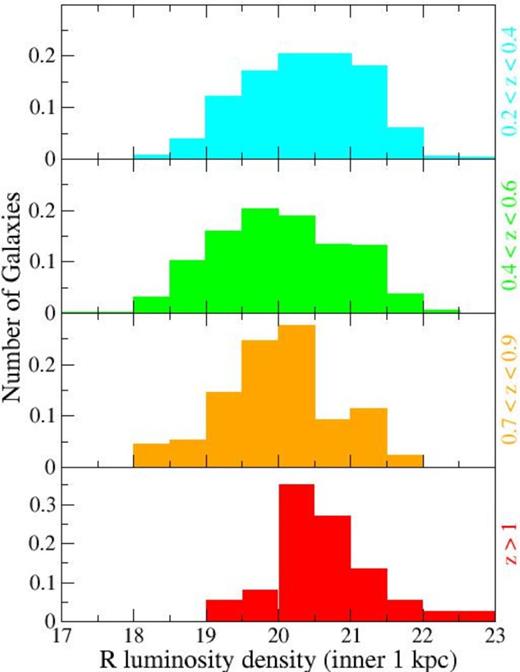
Central luminosity density (within the inner kpc) for galaxies in our samples. There is no strong evidence of an increase over z < 1 and therefore little evidence for bulge growth.
Consequently, it appears that the high central densities of the spheroidal components of the CRSGs are in place by z ∼ 1. The origin of the outer, younger, more metal-poor material is more uncertain: as an example, it may itself have been accreted through minor mergers at an earlier epoch (before z = 1.5), perhaps even during pre-processing of galaxies before they join the main cluster. From both the limited results on concentration obtained here and the arguments based on the work of Tacchella et al. (2015), it is likely that the spheroidal components of most of the 1 < z < 1.4 CRSGs are already in place. This would imply that the decrease in the contribution from disc-like components in the population over the 3–4 Gyr between z ∼ 1.4 and ∼0.5 was mainly or solely due to the fading or rearrangement of the discs and not from the build-up of a bulge component (or at least the central regions of any bulge). This evolution in the discs may be triggered by disc instabilities, tides, harassment, fly-bys and a series of other external and internal processes we are not in a position to explore here. A further indication that the morphological transformation may be due to changes in the disc is the concurrent evolution observed in the axial ratios and Sérsic indices, which tend to reinforce our impression that the spheroidal portion of these galaxies has been established at early times and only the younger, and perhaps more fragile, discs appear to be involved in the morphological changes we observe.
One result that does not directly follow from the strawman model is the (albeit small) increase in the typical size (Reff) of the CRSG population between z ∼ 1.4 and ∼0.6. If a disc fades and reddens relative to its bulge, with no large-scale change to the bulge structure it would be expected that the overall Reff would probably decrease (albeit by a modest amount) rather than increase, in the absence of any other morphological evolution. Given the small size of any evolution, it could be explained by other evolutionary effects in only a subset of the comparatively small ‘high’ and ‘very high’ subsamples. We note here that the strawman model does not account for this potential behaviour, but is certainly not currently ruled out by it. For instance, it is possible that any size evolution in the overall CRSG population could be driven by galaxies other than those which are evolving morphologically in the manner discussed here.
Alternatively, one may envisage the disc being disturbed, for instance by minor mergers or fly-bys, and then added on to the outer regions of the bulge, thus driving a modest increase in size and Sérsic index as structure is increased in the outer regions, and reducing the oblateness of galaxies. Such fly-bys would be frequent in the dense environment of clusters and may result in significant structural changes in haloes (Sinha & Holley-Bockelmann 2015). Disc instability would be another possibility (e.g. Shankar et al. 2013; Huertas-Company et al. 2015). In the model by Naab, Johansson & Ostriker (2009), for instance, galaxies are born as highly flattened objects and their discs are later on destroyed or rearranged by interactions and mergers with minor satellites (e.g. Quilis & Trujillo 2012) to form a more spheroid-dominated population. Several other mechanisms are possible, as discussed in the vast literature on size growth of spheroids, but we are not in a position here to speculate.
A clear improvement to the analysis presented here would be to carry out detailed two-component surface brightness fitting to CRSGs over the entire redshift range and perhaps beyond z ∼ 1.4 where the analysis may need to be extended to slightly bluer galaxies due to the increased influence of star formation in red sequence progenitors. This is not reliably achievable with the current HST data, especially at high redshift where the most changes are seen (cf. Cameron & Driver 2007). Deeper exposures could be obtained with HST. However, an equally important issue is to be able to resolve the galaxies on scales smaller than Reff in the reddest bands. Higher spatial resolution will allow the analysis to separate out any disc and bulge component and therefore to securely determine how much of the observed evolution is caused by bulge growth and how much to disc fading. This will be straightforwardly achievable with James Webb Space Telescope (JWST).
6 CONCLUSIONS
We have explored the morphological evolution of cluster red sequence galaxies using a large sample of such galaxies drawn from multiple clusters over the redshift range 0.2 < z < 1.4 split into four subsamples by redshift. Our previous work showed there were significant differences between the populations at 1 < z < 1.4 and z ∼ 0. Here we fill in details of their evolution over the intervening 9–10 Gyr. Our major findings are the following.
We confirm that the distribution in structural parameters of high-redshift cluster galaxies differs from those at lower redshift. At least a proportion of the population evolves morphologically having arrived on the red sequence subsequent to quenching of star formation.
The measurements indicate that this evolution largely ends by z ∼ 0.5–0.6, a lookback time of 5–6 Gyr and a likely 3–4 Gyr after quenching of star formation. This evolution is seen in the distribution of Sérsic parameters, axial ratios, sizes and colour gradients.
The evolution in each of these parameters indicates typical objects become less disc dominated with time, with the strength of any colour gradient (bluer on the outside) decreasing similarly. The data broadly fit a simple model where (thin) disc components fade and redden more quickly than their central bulges, straightforwardly explained by more recent quenching of star formation in the disc than in the bulge. The time-scale for this matches the 3–4 Gyr over which we can detect changes in the structural parameters. During this time the discs are required to thicken in order to explain the changing axial ratio distribution, agreeing with the time-scale for the expected tidal thickening of discs in clusters. The obvious implication of the model is that these initially disc-dominated galaxies are the progenitors of the passive S0 systems that populate (indeed dominate) the red sequence of intermediate- and low-redshift clusters at luminosities around L* and below (also see Chan et al. 2016; Lopes et al. 2016).
We confirm that the size growth in the population of red sequence galaxies in clusters is significantly less over the past 9–10 Gyr than that of similar mass passively evolving field galaxies. The data indicate that any growth is likely to occur at z > 0.6 as the size distributions of our two lower redshift subsamples appear indistinguishable.
While the decreasing prominence of any disc component could have a contribution from bulge growth over time, consideration of the fraction of the luminosity (mass) within the central 1 kpc of each galaxy indicates that at least to z ∼ 1 this is not a significant factor in the evolution of the measured structural parameters.
Although further similar HST data sets (with both rest-frame B- and R-band imaging) for z > 0.6 clusters would improve the statistical significance of some of these results, improvements in the interpretation of these results will only come from the ability to securely fit multicomponent surface brightness profiles to high-redshift samples. This will only be achievable through JWST imaging which will give sufficient signal-to-noise ratio and spatial resolution at the highest redshifts to separate the co-evolution of disc and bulge components in cluster red sequence galaxies.
This work is based on observations made with the NASA/ESA Hubble Space Telescope, and obtained from the Hubble Legacy Archive, which is a collaboration between the Space Telescope Science Institute (STScI/NASA), the Space Telescope European Coordinating Facility (ST-ECF/ESA) and the Canadian Astronomy Data Centre (CADC/NRC/CSA). Some of the data presented in this paper were obtained from the Mikulski Archive for Space Telescopes (MAST). STScI is operated by the Association of Universities for Research in Astronomy, Inc., under NASA contract NAS5-26555.
REFERENCES
SUPPORTING INFORMATION
Additional Supporting Information may be found in the online version of this article:
Please note: Oxford University Press is not responsible for the content or functionality of any supporting materials supplied by the authors. Any queries (other than missing material) should be directed to the corresponding author for the article.
