


Abstract
In earlier works, it was shown that the energy-dependent soft time lags observed in kHz quasi-periodic oscillations of neutron star low-mass X-ray binaries can be explained as being due to Comptonization lags provided a significant fraction (η ∼ 0.2–0.8) of the Comptonized photons impinge back into the soft photon source. Here we use a Monte Carlo scheme to verify if such a fraction is viable or not. In particular we consider three different Comptonizing medium geometries: (i) a spherical shell, (ii) a boundary layer like torus and (iii) a corona on top of an accretion disc. Two sets of spectral parameters corresponding to the ‘hot’ and ‘cold’ seed photon models were explored. The general result of the study is that for a wide range of sizes, the fraction lies within η ∼ 0.3–0.7, and hence compatible with the range required to explain the soft time lags. Since there is a large uncertainty in the range, we cannot concretely rule out any of the geometries or spectral models, but the analysis suggests that a boundary layer type geometry with a ‘cold’ seed spectral model is favoured over an accretion corona model. Better quality data will allow one to constrain the geometry more rigorously. Our results emphasize that there is significant heating of the soft photon source by the Comptonized photons and hence this effect needs to be taken into account for any detailed study of these sources.
1 INTRODUCTION
X-ray binaries are close binary systems where the compact object accretes matter from a companion star via an accretion disc. The compact object can be either a neutron star or a black hole, while the companion star is a main sequence one. The X-ray luminosity is usually generated in the inner accretion disc near to the compact object. There are two types of X-ray binaries, high-mass X-ray binaries (HMXBs) where the companion star is an O or B star, and low-mass X-ray binaries (LMXBs) where the companion star is a K or M star. The X-ray binaries are categorized into mainly two classes, transient and persistent, based on their long-term X-ray variability. They have in general two distinct spectral states, a high luminous soft state, which is dominated by a blackbody like emission, and a low luminous hard state, which is dominated by power-law emission. They also typically show a third intermediate or transitional state where the X-ray flux is highly variable on time-scale of milliseconds to seconds. The variability is sometimes of a quasi-periodic nature, and are termed as quasi-periodic oscillations (QPOs). In particular, neutron star LMXBs have millisecond variability and their kHz QPOs are positioned in definite regions on their colour–colour plots (Straaten, van der Klis & Mendez 2003; Altamirano et al. 2008). These QPOs occur during the soft to hard state transition (see e.g. Belloni, Mendez & Homan 2007); and they seem to have no long-term correlation with X-ray luminosity (Méndez et al. 1999; Misra & Shanthi 2004).
Important insights into the nature of these oscillations can be obtained by studying the fractional root mean square (rms) amplitude, and phase delay or time lag as a function of energy which depend on the type of QPO and typically show complex behaviour (see, for review, Tanaka & Shibazaki 1996; van der Klis 2000, 2006; Remillard & McClintock 2006). The energy dependence of the rms and time lag contain clues regarding the radiative processes that are involved in the QPO phenomena.
Spectral fitting reveals that thermal Comptonization is the main radiative mechanism for hard X-ray generation in X-ray binaries. In this process, the seed photons are Comptonized by a hot thermal electron cloud or corona. The thermal Comptonization process is generally characterized by three parameters, the seed photon source temperature Tb, the corona temperature Te and the optical depth of the medium τ or the average number of scattering 〈Nsc〉 that a photon would undergo (Sunyaev & Titarchuk 1980). 〈Nsc〉 depends on the geometry of the corona and for a given optical depth, it is generally difficult to compute analytically for arbitrary corona shapes. Since the dominant spectral component in X-ray binaries is due to thermal Comptonization, the energy-dependent rms and time lag of the QPOs may be related to the process. Indeed, the energy dependence of the rms and time lag for the lower kHz QPO can be explained in terms of a thermal Comptonization model, and moreover such an analysis can provide estimates of the size and geometry of the corona (Lee & Miller 1998; Lee, Misra & Taam 2001). In a more detailed work Kumar & Misra (2014) studied the expected energy-dependent time lags and rms for different kinds of driving oscillations such as in the seed photon temperature or in the coronal heating rate, while self-consistently incorporating the heating and cooling processes of the medium and the soft photon source. They showed that the observed soft lag for the lower kHz QPO could be obtained only when the driving oscillation is in the heating rate of the corona and if a substantial fraction, η, of the Comptonized photons impinge back into the soft photon source. However, the quantitative results obtained depend on the specific time-averaged spectral model used for the analysis. Typically in the Rossi X-ray Timing Experiment (RXTE), Proportional Counter Array (PCA) energy band of 3–20 keV, there are two spectral models namely the ‘hot’ and ‘cold’ seed photon models which are degenerate, i.e. they both equally fit the data of neutron star LMXBs (Mitsuda et al. 1984; White et al. 1986; Barret 2001; Di Salvo & Stella 2002; Lin, Remillard & Homan 2007; Cocchi, Farinelli & Paizis 2011). In, Kumar & Misra (2016, hereafter Paper I), we employed both these spectral models to infer the size of the medium and fraction of photons impinging on the soft seed source, η, for different QPO frequencies of the transient source 4U 1608−52. While both spectral models can explain the rms and time lag as a function of energy, the range of the size of the medium for the hot seed photon model 0.2–2.0 km is significantly different than when the cold seed photon model is used, 1–10 km. Moreover, we compared the measured soft lags between two broad energy bands versus kHz QPO frequency (Barret 2013) with the model predicted ones. We found that the width of medium L decreases with QPO frequency for the hot-seed model, but there is no such trend in cold-seed one, perhaps because the allowed range of the size is larger. For both models, we obtained the inferred ranges of L and η. Thus, it was shown that while interpreting the time lag of the kHz QPO as being due to Comptonization, can lead to estimates of the size of the medium, it is necessary to have a reliable time-averaged spectral model to do so.
A generic feature of the analysis was that since the observed time lags are soft, there needs to be a significant fraction, η > 0.2 of the Comptonizing photons to impinge back into the soft photon source. While in these earlier works it has been treated as a parameter, in principle, it should be computed for a given geometry. In this work, we endeavour to do so, by implementing a Monte Carlo method to trace the photons as they scatter, escape from the medium and impinge into the soft photon source. The motivation here is to compute η as a function of size and for different simple geometries. We will then compare the results with the constraints obtained in Paper I, to find if any of the geometries are more viable. We will neglect general relativistic effects and any bulk (including orbital) motion of the Comptonizing medium.
In the next section, we briefly discuss the scheme of the Monte Carlo method used for the thermal Comptonization process. In Section 3, η is computed for three different geometries of the Comptonizing system and in Section 5, the results are summarized and discuss.
2 MONTE CARLO METHOD
In a Monte Carlo method a photon is tracked as it enters the Comptonizing medium and scatters multiply till it leaves the medium. The process is repeated for a large number of photons to build up the statistics that would give the emergent spectrum as well as the direction of each outgoing photon. The technique has been in use for several decades now (for e.g. Sazonov & Sunyaev 2000; Zdziarski & Pjanka 2013). Pozdnyakov, Sobol & Sunyaev (1983) have extensively reviewed the Monte Carlo method for the thermal Comptonization process. The algorithm used in this work for the Monte Carlo method in the lab frame has been adopted from their paper and the specific scheme used is from the appendix of Hua & Titarchuk (1995).
Since our analysis is in the non-relativistic regime, i.e. the electron temperature, kTe, and the photon energies considered are ≪mec2, and that the size of the region is much larger than the scattering length, the diffusion limit is still valid. Thus, we can test the code with the analytical results obtained in this limit including the resultant spectrum from the Kompaneets equation (Kompaneets 1957). We test the code in three stages. First, we compute the average energy change for a monochromatic photon of frequency ν scattering once in a thermal medium, kTe which is expected to be |$\Delta E = (4kT_{\rm e}-h\nu )\frac{h\nu }{m_{\rm e}c^2}$|. We computed this average change in energy of the photon for different temperatures and found it to match with the above expectation. Next, for a spherical geometry, where the source of seed photons is located at the centre, we consider the average number of scatterings that a photon will undergo 〈Nsc〉 and the scattering number distribution. For such a spherical shape geometry, one can estimate in the diffusion limit that |$\langle N_{{\rm sc}}\rangle = \frac{\tau ^2}{2}$| and the peak of scattering distribution should be around ∼0.3τ2 (Sunyaev & Titarchuk 1980). We find these expected results for the Monte Carlo code, for e.g. for τ = 9.2, 〈Nsc〉 was found to be 41.4, and the peak of the distribution was around 25. Finally, we compare the output spectra of the code with the analytical ones and find a good match as shown in Fig. 1. Here, the medium temperature is fixed at kTe = 3.0 keV. The points with error bars are from the Monte Carlo results while the lines are the analytical solutions of the Kompaneets equation (as is described in Kumar & Misra 2014) in which the (τ2 + τ) term is equated with 〈Nsc〉. The curve marked 1 is for the case when the soft photon temperature kTb = 0.1 keV and τ = 9.2. For these values the spectrum around 1 keV should be of a power law form and that indeed is seen. The curve marked 3 is for the case when the soft photon temperature kTb = 1.0 keV and 〈Nsc〉 = 500. Here the emergent spectrum is a Wien peak as expected. The curve marked 2 is for the case when the soft photon temperature kTb = 1.0 keV and τ = 9.2 and the Monte Carlo spectrum matched well the analytical one. Thus in different regimes of Comptonization, the code gives expected results.
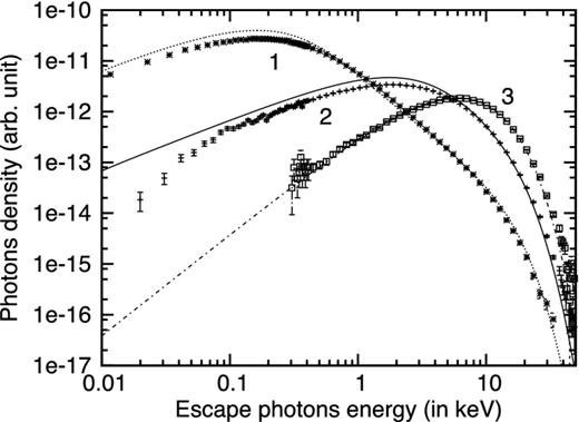
Spectra comparison of Monte Carlo results with analytic ones. Here the points with error bars are from Monte Carlo computations while the lines are from analytic solutions. The three curves represent three different regimes of Comptonization namely power law (1), intermediate (2) and Wien peak (3). In all three regimes the Monte Carlo technique produces results close to the analytical ones, validating the code being used.
3 ESTIMATING THE FRACTION |$\boldsymbol {\eta _{\rm e}}$| FOR DIFFERENT GEOMETRIES
As shown in Paper I, an important parameter that determines the nature of the energy-dependent time lag is the fraction of photons impinging back into the soft photon source. Perhaps a more physical quantity is the fraction in terms of photon energy, i.e. |$\eta _{\rm e} =\frac{\int n_{\gamma {\rm b}} (E) E \, {\rm d}E}{\int n_{\gamma } (E) E\, {\rm d}E}$|, where nγ(E) represents the photons that emerge from the Comptonizing medium, while nγb(E) represents those photons which impinge back into the source. Note that this energy weighted fraction ηe would be close to the photon fraction |$\eta =\frac{\int n_{\gamma {\rm b}} (E) \, {\rm d}E}{\int n_{\gamma } (E)\, {\rm d}E}$| as long as the emergent spectrum is not highly anisotropic. In other words, ηe ∼ η as long as the spectral shape of the photons going into the soft source nγb(E) is not very different from the average emergent spectrum nγ(E). In this section, our aim is to estimate ηe for different geometries using the Monte Carlo scheme.
As mentioned earlier, the spectra of neutron star LMXBs in the 3–20 keV band can be fitted by two degenerate models namely the ‘hot’ and ‘cold’ seed photon ones. The best-fitting spectral parameters for a given model also vary between different observations. In Paper I, we used spectral parameters for nine representative RXTE observations spanning a QPO frequency range of 500–900 Hz. In this work we consider two sets of spectral parameters which roughly correspond to the spectra when the QPO frequency is low (∼600 Hz) and high (∼800 Hz). This is done for both the ‘hot’ and ‘cold’ seed photon models. Table 1 lists the spectral parameters used where the ‘hot’ seed photon models are named Ia and Ib while the spectra corresponding to ‘cold’ seed photon model are named IIa and IIb. The Monte Carlo computations have been done for each of these four set of spectral parameters.
List of Comptonization spectral parameters used for the Monte Carlo code to compute ηe. The hot and cold seed photon models are represented by two sets of spectral parameters.
| Model | Index | Comptonization parameters | ||
|---|---|---|---|---|
| kTe (keV) | kTb (keV) | τ | ||
| Hot seed | Ia | 3 | 1 | 9 |
| Ib | 5 | 1 | 5 | |
| Cold seed | IIa | 3 | 0.4 | 9 |
| IIb | 5 | 0.4 | 5 | |
| Model | Index | Comptonization parameters | ||
|---|---|---|---|---|
| kTe (keV) | kTb (keV) | τ | ||
| Hot seed | Ia | 3 | 1 | 9 |
| Ib | 5 | 1 | 5 | |
| Cold seed | IIa | 3 | 0.4 | 9 |
| IIb | 5 | 0.4 | 5 | |
3.1 Spherical/hollow shell
We start with the simplest geometry depicted in Fig. 2, where the neutron star is covered by a spherical shell which Comptonizes photons from the surface of the neutron star. The radius of the neutron star is fixed at Rs = 10 km while the size of the shell L is taken as a parameter. Although perhaps not physical, we also consider for completeness, the possibility that the Comptonizing medium is a hollow shell having a vacant region of size RH between it and the neutron star (right-hand panel of figure). For both geometries, we define the optical depth τ in the radial direction such that the corresponding electron density ne is |$\frac{\tau }{\sigma _{\rm T} L}$|.

A cross-sectional view of the spherical shell (left-hand panel) and the hollow spherical shell (right-hand panel) geometry. The grey region is the Comptonizing medium of width L while the white region is the hollow/empty region of width RH. The black region represents the neutron star with radius RS.
In the Monte Carlo code, a photon is released from the surface of the neutron star and is tracked till it either escapes or impinges back to the surface. One expects that the fraction ηe will decrease with increasing L since the probability that a photon gets absorbed by the surface decreases. This is indeed the case as shown in Fig. 3 where the left-hand and middle panels show the computed ηe as a function of L for the four spectral parameters tabulated in Table 1. For comparison, the plots also show the range of η and L for the ‘cold’ and ‘hot’ seed photon models inferred by the energy-dependent rms and time lag of the kHz QPO (Paper I). Although the range of η and L is rather large due to the quality of the data, it is heartening to see that for this geometry the computed ηe fall within this range. If better quality data indicate a smaller ηe then perhaps such a geometry can be ruled out. Naturally, a hollow geometry would lead to lower values of ηe. The average number of scatterings 〈Nsc〉 increases with the gap size RH. However for RH ≈ 0.3RS 〈Nsc〉 varies from the spherical case by only 10 per cent and the emergent spectrum does not vary significantly. The right-hand panel of Fig. 3 shows this decrease of ηe versus the gap size RH for fixed values of L = 0.5 (solid line) and 1.0 km (dashed line).
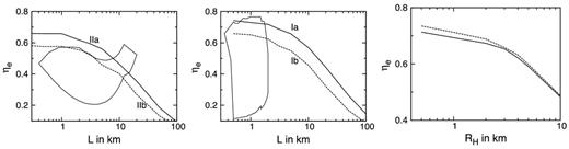
Variation of ηe versus size for the spherical shell geometry. The left-hand and middle panels show ηe variation with the size of the Comptonizing medium for the ‘cold’ seed photon model (left-hand panel) and for the ‘hot’ seed photon model (middle panel). The marking on the curves (Ia, Ib, IIa, IIb) represents the spectral parameters used for the computations as listed in Table 1. The closed curves represent the estimated range of η and size that are required to explain the soft time lag in the kHz QPO (Paper I). The right-hand panel shows the variation of ηe with the gap size RH for the hollow shell model for the hot seed photon model spectra Ib. The solid line is for L = 1 km while the dashed one is for L = 0.5 km.
3.2 Boundary layer geometry
The boundary layer is a region that connects the accretion disc to the neutron star surface, i.e. the accreting material makes a transition from centrifugal to pressure support near the star (e.g. Popham & Narayan 1995; Popham & Sunyaev 2001). Here, we approximate the geometry as shown in the left-hand panel of Fig. 4. We consider a rectangular torus surrounding the spherical neutron star. The radius of the neutron star is kept fixed at Rs = 10 km. The gap between the torus and the neutron star Rg is also fixed at a small distance of 50 m following Babkovskaia, Brandenburg & Poutanen (2008) who estimate that the maximum distance between the star surface and the layer is about 100 m. The width of the torus in the radial direction is taken to be a parameter LR while its half-height in the vertical direction is LH. This geometry allows for two definitions of the optical depth τ, one along the vertical (here τ is the half-height optical depth, i.e. the electron density in the torus is ne= |$\frac{\tau }{L_{\rm H} \sigma _{\rm T}}$|) and other in the radial direction and we do the analysis for both definitions. For the same optical depth defined in either fashion, the average number of scatterings 〈Nsc〉 is smaller by a factor of ∼1.5 than for the spherical shell case studied above. Hence we use a slightly higher values of τ, 10.4 and 5.8 instead of 9 and 5 mentioned in Table 1. We emphasize that these changes have little effect on the overall results.
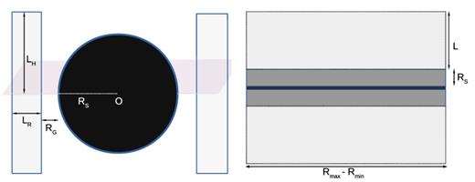
A cross-sectional view of the boundary layer geometry (left-hand panel) and the accretion disc/corona geometry (right-hand panel). For the boundary layer geometry the Comptonizing medium is assumed to be a torus with a rectangular cross-section (light grey) surrounding the neutron star (black). For the accretion disc corona geometry the Comptonizing medium lies above and below the accretion disc.
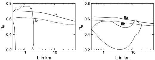
We first consider the case when the optical depth is defined along the vertical direction and we explore the variation of ηe with the vertical height LH for fixed radial extent LR and for different spectral parameters. This is shown in Fig. 5 where the top panels are for LR = 1 km while the bottom ones are for LR = 20 km. The left-hand panels are for the ‘hot’ seed photon model while the right ones are for the ‘cold’ seed photon one. The contours mark the estimated ranges of η and L from Paper I. Fig. 6 is the same as Fig. 5 except that now the optical depth is defined along the horizontal direction and the top and bottom panels are for fixed values of LH = 1 and 20 km, respectively. It is clear from both these figures that for a wide range of sizes and spectral models, the fraction ηe falls within the range required to explain the energy-dependent rms and time lags of the kHz QPOs.
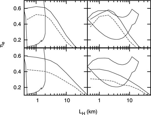
ηe as a variation of size for the boundary layer geometry when the optical depth is defined along the vertical direction. The top and bottom two panels are for the case when the horizontal width is taken to be LR = 1 and 20 km, respectively. The left- and right-hand panels are for the hot and cold seed photon models. The solid and dashed lines are for two corresponding spectral parameters. The closed curves show the allowed range of η and size obtained in Paper I.

ηe as a variation of size for the boundary layer geometry when the optical depth is defined along the radial direction. The top and bottom two panels are for the case when the vertical height is taken to be LH = 1 and 20 km, respectively. The left- and right-hand panels are for the hot and cold seed photon models. The solid and dashed lines are for two corresponding spectral parameters. The closed curves show the allowed range of η and size obtained in Paper I.
3.3 Disc–corona geometry
We next consider a third possible geometry, i.e. of an optically thick accretion disc sandwiched by a hot corona as shown in the right-hand panel of Fig. 4. The height of the corona is taken to be L while the disc and the corona above is considered to span from an inner radius of Rmin to Rmax (as shown in the right-hand panel of Fig. 4). The optical depth τ is defined along the vertical direction. For computational purposes we have introduced a thickness of the disc of Rs = 0.2 km but the results, as expected, are insensitive to this value. In fact the determining parameter here is the ratio of the height of the corona to the annular width of the disc Rmax − Rmin. Thus we fix Rmax − Rmin = 10 km and vary L. While 〈Nsc〉 changes with increasing L, the variation is not significant for the parameters chosen for this work. Hence, for this geometry, we have used the value of τ as given in Table 1.
In Fig. 7, we plot the fraction ηe versus height L for different spectral parameter values and as before compare with ranges obtained in Paper I. As expected, there is only a weak dependence of ηe on L and it has a rather large value of ∼0.7. In fact for the ‘cold’ seed photon case ηe is marginally larger than the maximum value obtained in Paper I. This seems to suggest that for this case at least, such a disc–corona geometry is unfavourable. However, given the large uncertainties it is difficult to make concrete statements. Nevertheless, our results show that for such a geometry the value of ηe is expected to be large, more or less independent of the thickness of the corona.
ηe as a function of the coronal width L for the accretion disc–corona geometry. Here the extent of the disc Rmax − Rmin = 10 km. The left- and right-hand panels are for the hot and cold seed photon models. The solid and dashed lines are for two corresponding spectral parameters. The closed curves show the allowed range of η and size obtained in Paper I.
4 SUMMARY AND DISCUSSION
Using a Monte Carlo scheme, we estimate the fraction of Comptonized photons that impinge back into the seed photon source η for different geometries and spectral parameters relevant to neutron star LMXBs. The primary motivation was that to explain the observed soft lags in KHz QPOs, one needed to invoke a large value η in the range of 0.2–0.6 and it was important to find out if this range can be achieved for any reasonable accretion geometry.
We consider three kinds of geometries for the Comptonizing medium which are (i) a spherical shell around the neutron star, (ii) a boundary layer system where the medium is taken to be a rectangular torus around the star and (iii) a corona sandwiching a thin accretion disc. We consider different sizes for the medium and a range of spectra parameters. In particular we consider two extreme cases of spectral parameters for the two degenerate spectral models which are called the hot and cold seed photon models.
Our basic result is that for a wide range of reasonable sizes and spectral parameters, the values of ηe computed by the Monte Carlo method lie within 0.2–0.8 and hence are compatible with the values used in Paper I to explain the soft time lags of the kHz QPOs. Since the range of η and size inferred from fitting the time lags are rather broad, we cannot concretely rule out any of the three geometries considered. However, it seems that the boundary layer geometry can have η values more in line with what is required and the disc–corona geometry produces η values which are marginally larger. Our results show that it is possible to constrain the geometry of the system if high quality data for energy-dependent time lags are available. We look forward to data from the recently launched satellite ASTROSAT1(Agrawal 2006; Singh et al. 2014), which might provide such high quality data. Perhaps it would then be warranted to consider other complexities such as the seed photons for the boundary layer case may be produced in the accretion disc rather than the neutron star surface or that the corona on top of the accretion disc maybe in the form of inhomogeneous clumps rather than being a uniform medium. Also, not all the photons that impinge back into the source, will be absorbed and one needs to solve the radiative transfer equations self-consistently to find the fraction reflected. This reflected emission will have light travel time delays which may significantly affect the time lags between different energy bands.
Finally, it is interesting to note that for the geometries considered here a significant fraction of the photons impinge back into soft photon source. This effect needs to be taken into account in any detailed study of these X-ray binaries.
NK thanks CSIR/UGC for providing support for this work.
REFERENCES
