


Abstract
The next Galactic supernova is expected to bring great opportunities for the direct detection of gravitational waves (GW), full flavour neutrinos, and multiwavelength photons. To maximize the science return from such a rare event, it is essential to have established classes of possible situations and preparations for appropriate observations. To this end, we use a long-term numerical simulation of the core-collapse supernova (CCSN) of a 17 M⊙ red supergiant progenitor to self-consistently model the multimessenger signals expected in GW, neutrino, and electromagnetic messengers. This supernova model takes into account the formation and evolution of a protoneutron star, neutrino-matter interaction, and neutrino transport, all within a two-dimensional shock hydrodynamics simulation. With this, we separately discuss three situations: (i) a CCSN at the Galactic Center, (ii) an extremely nearby CCSN within hundreds of parsecs, and (iii) a CCSN in nearby galaxies within several Mpc. These distance regimes necessitate different strategies for synergistic observations. In a Galactic CCSN, neutrinos provide strategic timing and pointing information. We explore how these in turn deliver an improvement in the sensitivity of GW analyses and help to guarantee observations of early electromagnetic signals. To facilitate the detection of multimessenger signals of CCSNe in extremely nearby and extragalactic distances, we compile a list of nearby red supergiant candidates and a list of nearby galaxies with their expected CCSN rates. By exploring the sequential multimessenger signals of a nearby CCSN, we discuss preparations for maximizing successful studies of such an unprecedented stirring event.
1 INTRODUCTION
Core-collapse supernovae (CCSNe) have been an active topic of research in theoretical and observational astrophysics for many decades. In recent years, hundreds of CCSNe have been discovered every year, mostly in distant galaxies (e.g. Sako et al. 2008; Leaman et al. 2011). However, these extragalactic CCSNe only provide a very indirect probe of the core-collapse process, and as a result, basic questions such as the mechanism by which CCSN explode still remains a mystery (for reviews, see e.g. Kotake, Sato & Takahashi 2006; Janka 2012). CCSNe in our Milky Way and neighbouring galaxies, while rare, provide the opportunity to study CCSNe with a suite of new observables, including neutrinos (e.g. Scholberg 2012), gravitational waves (GW; e.g. Ott 2009; Kotake 2013), and nuclear gamma rays (e.g. Gehrels, Leventhal & MacCallum 1987; Horiuchi & Beacom 2010). These are poised to more directly reveal the secrets laying deep inside the stellar photosphere.
Neutrinos and GWs in particular provide unique probes of the explosion mechanism in realtime. Multiple neutrino detectors capable of detecting CCSN neutrinos are currently in operation. The best suited is Super-Kamiokande (Super-K) which is expected to collect a rich data set of neutrino events from future Galactic CCSNe, while IceCube also has equal statistical detection potential even though IceCube cannot resolve individual neutrino events. Smaller detectors with sensitivity to CCSN neutrinos include, e.g. Baksan, Borexino, DayaBay, HALO, KamLAND, LVD, MiniBooNE, and NOνA (for their detection potentials, see e.g. recent review Mirizzi et al. 2016). In the near-future, the Jiangmen Underground Neutrino Observatory (JUNO; Li 2014) will augment Super-K and IceCube, and with future experiments such as Hyper-Kamiokande (Hyper-K; Abe et al. 2011) and Deep Underground Neutrino Experiment (DUNE; Acciarri et al. 2015), neutrino event statistics and neutrino flavour information will be dramatically improved. GW detectors such as Advanced LIGO (aLIGO), Advanced Virgo (adVirgo), and KAGRA are expected to be able to detect CCSN GW out to a few kpc from the Earth, while future detectors such as the Einstein Telescope (ET) can reach the entire Milky Way.
In order to exploit these potentials, a multimessenger observing strategy is necessary. In this context, the neutrino signal is particularly important. The neutrino emission in fact starts before the core collapse even begins. Neutrinos emitted during the final states of silicon burning can reach ∼5 × 1050 erg for a massive star (Arnett et al. 1989), which can be detected by Hyper-K out to a few kpc away (Odrzywolek, Misiaszek & Kutschera 2004), thereby providing an early warning signal. During the first ∼10 s after the core collapse, a copious ∼3 × 1053 erg of energy is emitted as neutrinos as was confirmed in SN 1987A (Bionta et al. 1987; Hirata et al. 1987; Sato & Suzuki 1987).
In addition to signalling unambiguously the occurrence of a nearby core collapse, the detected neutrinos will point to the location of the core collapse within an error circle of a few to ten degrees in the sky (Beacom & Vogel 1999; Bueno, Gil Botella & Rubbia 2003; Tomas et al. 2003). This pointing information is particularly important for electromagnetic signals, which remain a crucial component of studies of CCSNe in the Milky Way and nearby galaxies. A few hours to days after the core collapse, the supernova shock breaks out of the progenitor surface, suddenly releasing the photons behind the shock in a flash bright in UV and X-rays, known as shock breakout (SBO) emission (Matzner & McKee 1999; Blinnikov et al. 2000; Tominaga et al. 2009; Gezari et al. 2010; Kistler, Haxton & Yksel 2013). Although the SBO signal provides important information about the CCSN, such as the radius of the progenitor, detection is difficult because of its short duration. Knowing where to anticipate the signal will dramatically improve its detection prospects. In addition to the SBO, more traditional studies of CCSN properties (e.g. energy, composition, velocity) and its progenitor are important diagnostics of a CCSN, and a well-observed early light curve is important for accurate reconstruction of the CCSN evolution (e.g. Tominaga et al. 2011).
Already, various aspects of multimessenger physics of Galactic and nearby CCSNe have been investigated. For example, signal predictions of neutrino and GW messengers have been investigated by many authors. In particular, the first ∼500 ms following core collapse is thought to be critical for a successful explosion, and has been studied with three-dimensional (3D) hydrodynamics and three-flavour neutrino transport by various authors (e.g. Kuroda, Kotake & Takiwaki 2012; Hanke et al. 2013; Ott et al. 2013; Tamborra et al. 2014). On the other hand, the long-term neutrino emission characteristics have been investigated by several groups based on spherically symmetric general relativistic simulations using spectral three-flavour Boltzmann neutrino transport (e.g. Fischer et al. 2010). Similarly, while there are a number of multidimensional core-collapse simulations with GW predictions (e.g. Müller, Janka & Wongwathanarat 2012; Kuroda, Takiwaki & Kotake 2014; Yakunin et al. 2015), detailed detectability studies have been limited (see however, Gossan et al. 2016; Hayama et al. 2015). Leonor et al. (2010) have discussed utilization of a joint analysis of GW and neutrino data, particularly for electromagnetically dark (or failed) CCSNe. The importance of the SBO and their connections to multimessenger observations have been investigated by e.g. Kistler et al. (2013). Recently, Adams et al. (2013) revisited the investigation of dust attenuation of Galactic CCSNe. Using modern models of the Galactic dust distribution, they present the distributions of the observed V band and near-infrared (NIR) band magnitudes of Galactic CCSNe. They also emphasize the importance of neutrino warning and pointing, as well as the need for a wide-field IR detector for ensuring the detection of the early CCSN light curve.
In this paper, we revisit the implementations of multimessenger probes of CCSNe. We improve upon previous studies in several ways. First, we self-consistently determine predictions of neutrinos, GW, and electromagnetic signals from a CCSN based on a long-term two-dimensional (2D) axisymmetric simulation (Nakamura et al. 2015; Nakamura et al., in preparation). To focus on the most common Type IIP supernova, we adopt a non-rotating 17 M⊙ red supergiant star (RSG) with solar metallicity. The simulation gives neutrino and GW signals for the first ∼7 s after core bounce. We use the ensuing physical parameters (the radius and mass of the central remnant, the mass of synthesized nickel, and the explosion energy) to estimate the electromagnetic light curve. The time-sequence of multimessenger signals is summarized in Fig. 1. The pre-CCSN neutrino emission of Odrzywolek et al. (2004), the neutrino burst and gravitational energy release predicted directly from the numerical simulation, and the analytic bolometric light curve of SBO, plateau, and tail signals are shown and labelled. The neutrino burst luminosity is extrapolated up to 200 s based on the gravitational energy release rate from the shrinking protoneutron star (PNS). The GW energy emission rate is estimated using a quadrupole formula (Finn & Evans 1990; Müller, Janka & Marek 2013).
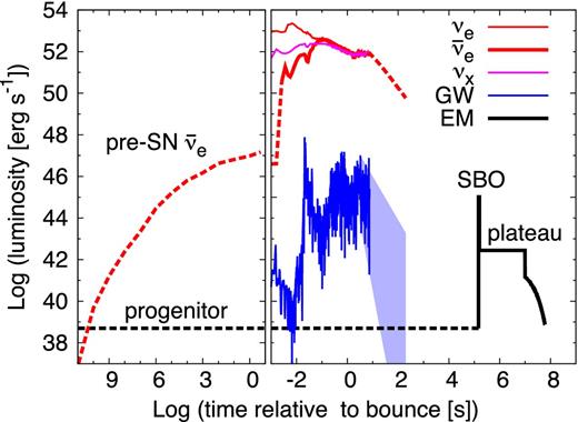
Time sequence for neutrino (red lines for νe and |$\bar{\nu }_e$| and magenta line for νx; νx represents heavy lepton neutrino νμ, ντ, |$\bar{\nu }_\mu$|, or |$\bar{\nu }_\tau$|), GW (blue line), and electromagnetic (EM, black line) signals based on our neutrino-driven core-collapse simulation of a non-rotating 17 M⊙ progenitor. The solid lines are direct or indirect results of our CCSN simulation, whereas the dashed lines are from literatures or rough speculations. The left-hand (right-) panel x-axis shows time before (after) core bounce. Emissions of pre-CCSN neutrinos as well as the core-collapse neutrino burst are shown as labelled. For the EM signal, the optical output of the progenitor, the SBO emission, the optical plateau, and the decay tail are shown as labelled. The GW luminosity is highly fluctuating during our simulation and the blue shaded area presents the region between the two straight lines fitting the high and low peaks during 3–5 s post-bounce. The hight of the curves does not reflect the energy output in each messenger; total energy emitted after bounce in the form of antielectron neutrino, photons, and GW is ∼6 × 1052 erg, ∼4 × 1049 erg, and ∼7 × 1046 erg, respectively. See the text for details.
In addition, we investigate tasks aimed at aiding the prospects of ensuring multimessenger signal detections of a future CCSN. For this purpose, we separately consider CCSN occurring in three distance regimes: we consider a CCSN occurring extremely nearby (less than 1 kpc away), at the Galactic Center (∼10 kpc, the most likely distance for a Galactic CCSN), and a CCSN in neighbouring galaxies (within several Mpc). Although neutrino detection can unambiguously indicate a core-collapse event, prompt and precise pointing information is needed for the electromagnetic community to fully exploit the advanced warning. In cases where this fails, either due to the electromagnetic signal appearing too quickly or the neutrino statistics limiting pointing precision, telescopes could resort to searching a pre-compiled list of potential targets. This is particularly useful in the case of CCSNe in nearby galaxies, whose expected neutrino event rates do not provide a compelling angular pointing. To these ends, we compile a list of known Galactic red supergiant candidates in the vicinity of the Earth, as well as a list of nearby galaxies with estimates of their CCSN rates.
The detectability of multimessenger signals are summarized in Table 1. The rows show the multimessenger signals, while the columns show three distance regimes. Names in italic denote future detectors. For neutrinos, only the dominant channels are shown: |$\bar{\nu }_e$| for Super-K, Hyper-K, and JUNO, and νe for DUNE. The detectors however have other channels that allow further spectral and flavour information to be extracted (for recent discussions, see e.g. Laha & Beacom 2014; Laha, Beacom & Agarwalla 2014). In particular, the neutral current events at liquid scintillator detectors such as JUNO hold the important capability to measure the heavy lepton flavour neutrinos (Beacom, Farr & Vogel 2002; Dasgupta & Beacom 2011). One important thing is enhancement of detectability by combining the signals. For example, we demonstrate that the information of the core bounce timing provided by neutrinos can be used to improve the sensitivity of GW detection. Importantly, this increases the GW horizon from some ∼2 to ∼8.5 kpc (based on our numerical model), which opens up the Galactic Center region to GW detection even for non-rotating progenitors [GW signals from collapse of rapidly rotating cores are circularly polarized (Hayama et al. 2016) and significantly stronger (e.g. Kotake 2013)].
Detectable signals, detectors, and their horizons.
| Extremely nearby event @ O(1 kpc) | Galactic event @ O(10 kpc) | Extragalactic event @ O(1 Mpc) | |||||
|---|---|---|---|---|---|---|---|
| (see Section 4) | (see Section 3) | (see Section 5) | |||||
| Signals | Detector | Horizon | Detector | Horizon | Detector | Horizon | |
| Neutrino | Pre-SN |$\bar{\nu }_{\rm e}$| | KamLand | <1 kpc | – | – | ||
| HK (20XX-) | <3 kpc | ||||||
| |$\bar{\nu }_{\rm e}$| burst | SK | Galaxya | SK | Galaxy | HK | <a few Mpc | |
| |$\bar{\nu }_{\rm e}$| burst | JUNO (201X-) | Galaxy | JUNO | Galaxy | – | ||
| νe burst | DUNE (20XX-) | Galaxy | DUNE | Galaxy | – | ||
| GW | Waveformc | H-L-V-Kd | <several kpc | ||||
| detection | H-L-V-K | ≲8.5 kpc | ET (20XX-) | ≲100 kpc | |||
| EM | Optical | <1 m class | 1–8 m classb | <1 m class | |||
| NIR | <1 m class | <1 m class | <1 m class | ||||
The paper is organized as follows. In Section 2, we summarize our setup. We describe our core-collapse simulation, methods for calculating multimessenger signals, and summarize the detectors we consider and the method for determining signal detections. We discuss the case of a CCSN in the Galactic Center in Section 3, the case of an extremely nearby CCSN in Section 4, and the case of a CCSN in neighbouring galaxies in Section 5. Sections 3–5 are all similarly organized in the following way: descriptions of the multimessenger signals separately, followed by a discussion of the merits and the ideal procedures for their combination. In Section 6, we conclude with an overall discussion and summary of our results.
2 SETUP
In this section, we describe the setup of exploring multimessenger signals from CCSNe. We first describe the setup of our numerical CCSN calculation, followed by how neutrino, GW, and optical signals are calculated. We then discuss multimessenger detector considerations.
2.1 Supernova model
The basis of our CCSN model is a long-term simulation of an axisymmetric neutrino-driven explosion initiated from a non-rotating solar-metallicity progenitor of Woosley, Heger & Weaver (2002) with zero-age main sequence (ZAMS) mass of 17 M⊙. This progenitor model has a radius 958 R⊙ and mass 13.8 M⊙ at the onset of gravitational collapse of the iron core. This progenitor retains its hydrogen envelope and is classified as a RSG. It is therefore expected to explode as Type II supernova.
The numerical code we employ for the core-collapse simulation is the same as found in Nakamura et al. (2015), except for some minor revisions. The spatial range considered in Nakamura et al. (2015) was limited to 5000 km from the centre. For the current study, we extend this to 100 000 km in order to study the late-phase evolution. This outer boundary corresponds to the bottom of the helium layer, and the interior includes 4.1 M⊙ of the progenitor. The model is computed on a spherical coordinate grid with a resolution of nr × nθ = 1008 × 128 zones.
For electron and anti-electron neutrinos, we use the isotropic diffusion source approximation (IDSA; Liebendörfer, Whitehouse & Fischer 2009), taking 20 energy bins with an upper bound of 300 MeV. Regarding heavy-lepton neutrinos, we employ a leakage scheme. In the high-density regime, we use the equation of state (EOS) of Lattimer & Swesty (1991) with a nuclear incompressibility of K = 220 MeV. At low densities, we employ an EOS accounting for photons, electrons, positrons, and ideal gas contribution from silicon. During our long-term CCSN simulation, we follow explosive nucleosynthesis by solving a simple nuclear network consisting of 13 alpha-nuclei. Feedback from the composition change to the EOS is neglected, whereas the energy feedback from the nuclear reactions to the hydrodynamic evolution is taken into account, as in Nakamura et al. (2014).
Fig. 2 shows time evolution of shock radius, Rsh, and explosion energy, Eexp. Here, the explosion energy is estimated by adding up the kinetic, internal, and gravitational energies in all zones where the sum of these energies and radial velocity are positive. This CCSN model successfully revives its shock at 296 ms after bounce and the shock reaches the bottom of the helium layer at the end of our simulation at 6.77 s. At the termination of the simulation, the explosion energy is 1.23 × 1051 erg and the mass of 56Ni in unbound material (summed up over the zones in the same manner as Eexp) is 0.028 M⊙.
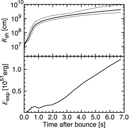
Time evolution of shock radius (top panel) and explosion energy (bottom panel). For shock radius, the maximum, mean, and minimum are shown as separate lines from top to bottom.
Fig. 3 visualizes the entropy distribution at four time snap shots. The formation of hot bubbles (the regions coloured by red in top-left panel of Fig. 3) is clear evidence of neutrino-driven convection, which revives the stalled bounce shock by the (so-called) neutrino-driven mechanism (Bethe 1990). In our model, the runaway expansion of the stalled shock initiates at about 200 ms post-bounce. In Fig. 3, the shock front (white contours) exhibits a dipolar deformation along the poles, as previously identified in 2D simulations (Bruenn et al. 2013; Summa et al. 2016), with the average shock radii becoming bigger with time (from top-left to bottom-right panel). After the shock passes the carbon core, the shape of the bipolar explosion (occurring stronger towards the north pole than the south pole, as seen in the bottom-right panel of Fig. 3) is kept nearly unchanged, and the shock expands rather in a self-similar fashion from thereon.
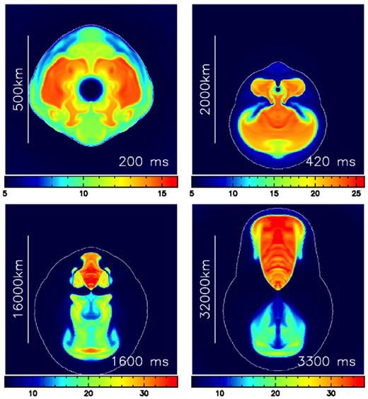
Entropy distributions in units of kB per baryon for the CCSN model at four selected post-bounce times indicated in the bottom-right corners. The white contour represents the shock front. Note the different scales in each panel.
2.2 Limitations of our model
Throughout this paper, we use the CCSN model described in the above section. The properties of CCSN model, however, depend on the structure of progenitor stars as well as input physics in simulations. Neutrino luminosity, for example, changes for different mass (or ‘compactness’) of progenitors and different choice of EOS (O'Connor & Ott 2013; Nakamura et al. 2015). Our simulations for 101 progenitor models with solar metallicity, employing the same numerical scheme and EOS as the current study, show diverse neutrino luminosities; 1.0–3.5 × 1052 erg s−1 at 0.5 s for anti-electron neutrino, 17 M⊙ model lying in between (1.7 × 1052 erg s−1). Note that the mass of the progenitor (17 M⊙) is not extreme and the EOS we use is widely accepted to CCSN modellers.
Numerical results also depend on unphysical variables, such as spatial resolution of simulations. We have tested the effects of angular resolution of spatial grid on CCSN properties. Besides a model with fiducial resolution of 128 angular zones, we used three additional models having 192, 256, and 320 angular zones. The numerical setup of the models was identical to the description in Section 2.1. For these models, differences in the shock dynamics as well as CCSN properties like explosion energy were observed as expected. Explosion energy, gravitational mass of PNS, and nickel mass in unbound material, estimated at 5.5 s after bounce, range in Eexp = 0.42–0.98 × 1051 erg, MPNS = 1.78–1.91 M⊙, and MNi = 0.013–0.025 M⊙, respectively. Our resolution study does not show any converging results and the resolution changes do not produce uniform trend, which is consistent with recent 2D results by Summa et al. (2016). It implies the strong influence of stochastic turbulent motions behind the shock front and difficulty in predicting any definitive CCSN properties given a progenitor structure.
What we present in this paper is just one example of simulated CCSNe, but it is quite important to discuss multimessenger signals focusing on one concrete example modelled by the state-of-the-art calculation.
2.3 Multimessenger emissions
We study three kind of multimessenger signals from the CCSN: neutrinos, GWs, and electromagnetic waves. Below, we briefly summarize the modelling of each signal, keeping the details in Appendix A.
Neutrinos. Neutrino signals are a direct outcome of our CCSN simulation which takes account neutrino transport in a self-consistent way. After emission from the collapsed core, neutrinos undergo flavour conversions during propagation to the Earth. In general, neutrino oscillation varies during the core-collapse evolution, and also depends on the neutrino mass hierarchy. Additional flavour mixing is induced by the coherent neutrino–neutrino forward scattering potential (for a review, see e.g. Duan, Fuller & Qian 2010; Mirizzi et al. 2016), and exact predictions of collective flavour transformation in the post-bounce environment, and when it will apply, and at what energies, are still under debate. Therefore, we consider as a simple scenario the Mikheyev–Smirnov–Wolfenstein (MSW) matter effects in the normal and inverted mass hierarchy, as well as a no-mixing and a full flavour swap scenario. While these scenarios are not equality realistic, they are aimed to cover the extremes (see Appendix A1 for details).
Gravitational waves. We extract the GW signal from our simulations using the standard quadrupole formula (e.g. Misner, Thorne & Wheeler 1973). For numerical convenience, we employ the so-called first-moment-of-momentum-divergence (FMD) formalism proposed by (Finn & Evans 1990, see also modifications in Murphy, Ott & Burrows 2009; Müller, Janka & Marek 2013). The angle between the symmetry axis in our 2D simulation and the line of sight of the observer is taken to be π/2 to maximize the GW amplitude (see Appendix A2 for details).
Electromagnetic signals. The first electromagnetic signal from the CCSN is the emission from SBO, followed by the characteristic plateau phase for Type IIP supernovae. Given the large difference in time-scales involved in our CCSN model (∼7 s) and the emergence of the SBO signal (a few minutes to a day), it is difficult for the current simulations of core collapse to directly reproduce the electromagnetic signals. Therefore, we use the final physical parameters of our simulation and employ analytic expressions for the luminosity and duration in SBO (Matzner & McKee 1999), and in the plateau phase (Popov 1993, see Appendix A3 for details).
2.4 Detector considerations
Below, we summarize the detectors setup assumed in this paper. In this paper, we will consider CCSNe at three distance regimes: occurring at the Galactic Center (Section 3), a very nearby location (Section 4), and extragalactic distances (Section 5). As we discuss in the subsequent sections, the necessary detector depends strongly on these distance regimes.
Neutrinos. We consider two water Čerenkov neutrino detectors, Super-K1 and its successor Hyper-K (Abe et al. 2011). Super-K has a fiducial volume of 32.5 kton in neutrino burst mode with a low-energy threshold of 3 MeV. For Hyper-K, we assume a burst-mode fiducial volume of 740 kton and an energy threshold of 7 MeV (Abe et al. 2011). The main detection channel is of |$\bar{\nu }_e$| with inverse-beta decay (IBD), which provides good kinematic but poor angular information of the incoming neutrinos (Vogel & Beacom 1999). We thus also consider electron scattering, which is sensitive to all neutrino flavours and is forward peaked (Vogel & Engel 1989). Details are included in Appendix A1.
Gravitational waves. We consider a network of interferometric GW detectors consisting of four detectors: aLIGO2 Hanford and Livingston, adVirgo,3 and KAGRA4 at their geophysical locations (H-L-V-K). For each detector, the noise spectrum is taken from Wen & Schutz (2005), Hild et al. (2009), and Aso et al. (2013), and we assume sensitivities that are expected to be realized by the year 2018. The detection of the gravitational waveform from a CCSN is determined using this global network of GW detectors by the coherent network analysis (Klimenko et al. 2005; Hayama et al. 2007; Sutton et al. 2010; Hayama et al. 2015). The coherent network analysis was introduced by Gürsel & Tinto (1989), the basis of which is to reconstruct arbitrary gravitational waveforms by linear combination of data from GW detectors. For the signal detection, reconstruction, and source identification, we perform Monte Carlo simulations using the RIDGE pipeline (see Hayama et al. 2007, for more details).
Electromagnetic signals. We consider electromagnetic observations in optical and NIR wavelengths. For detection of the electromagnetic signals, interstellar extinction proves to be critical (Adams et al. 2013). Since NIR wavelengths are only mildly affected by the extinction, Galactic CCSNe can be detected with small-size NIR telescopes. On the other hand, the optical brightness is significantly attenuated by dust extinction, which depends on the location of the CCSN event. In addition, since the positional localizations by GW and neutrino detections are typically larger than a few degree, wide-field capability is also crucial not to miss the very first electromagnetic signals. Therefore, for optical telescopes, we consider various sizes of wide-field telescopes/facilities, such as the All-Sky Automated Survey for SuperNovae (ASAS-SN; Shappee et al. 2014), Evryscope (Law et al. 2015), Palomar Transient Factory (PTF; Law et al. 2009; Rau et al. 2009), Pan-STARRS1 (PS1; e.g. Kaiser et al. 2010), Subaru/Hyper Suprime-Cam (HSC; Miyazaki et al. 2006, 2012), and Large Synoptic Survey Telescope (LSST; Ivezic et al. 2008).
3 GALACTIC CENTER SUPERNOVAE
3.1 Neutrino signal
We obtain the values of (Lν, 〈Eν〉, α) for |$\nu = (\nu _e, \bar{\nu }_e, \nu _x)$| from our core-collapse simulation,5 and show the event rate per 1 ms bin expected for a 8.5 kpc event at the Hyper-K detector in Fig. 4. The thick blue and thin red lines denote inverse beta and e−-scattering events, respectively. The central solid lines denote MSW mixing, while the upper and lower lines denotes the no-mixing and full-mixing cases, respectively. The time-integrated number of events is 328 000–329 000 inverse-beta events and 11 300–11 700 e− scattering events.
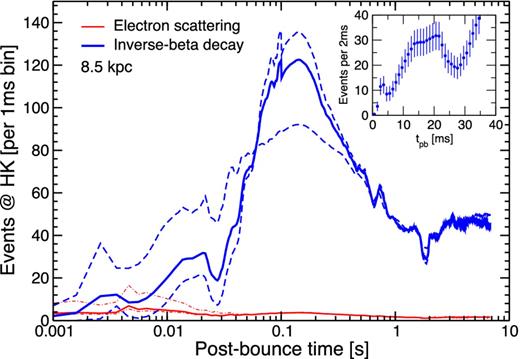
Expected neutrino events at Hyper-K in 1 ms time bins, for a Galactic CCSN at a distance of 8.5 kpc. Inverse-beta events are shown by thick blue lines, while the lower thin red lines denote electron scattering events. For each, the three lines show three neutrino mixing scenarios: (i) MSW mixing (central solid lines), (ii) no mixing (upper lines), and (iii) full flavour swap (lower lines). This is done to show the range of possible mixing, accounting for both mass hierarchies, MSW, and collective neutrino oscillations. The MSW mixing line represents normal (inverted) mass hierarchy for |$\bar{\nu }_e$| (νe). The no mixing assumes the observed electron neutrinos are entirely composed of the same flavour at source (i.e. |$\bar{\nu }_e = \bar{\nu }_e^0$| and |${\nu }_e = {\nu }_e^0$|), while the full swap assumes they are entirely exchanged with the heavy flavour states at source (i.e. |$\bar{\nu }_e = {\nu }_x^0$| and |${\nu }_e = {\nu }_x^0$|); see Appendix A1 for details. The inset shows the first 40 ms of the IBD signal at Hyper-K, shown in 2 ms bins, for the MSW mixing case. The error bars are root-N Poisson errors.
The high-statistics light curve will enable various studies, such as probes of the standing accretion shock instability (SASI; see e.g. Foglizzo et al. 2015, for a recent review) that affect the luminosities and energies of the emitted neutrinos. The detectability of SASI has been explored by various studies focusing on both Hyper-K and IceCube for Galactic CCSNe (Lund et al. 2010, 2012; Tamborra et al. 2013, 2014). Our particular progenitor explodes predominantly by neutrino-driven convection and hence the SASI modulated signal is weak. The neutronization burst will also allow unique probes of the core collapse (Kachelriess et al. 2005). During this phase, the collapse is spherical enough that the bulb model, i.e. neutrinos emitted from a sharp spherical surface, is a reasonable approximation for neutrino mixing calculations (e.g. Cherry et al. 2012).
The time of core bounce can be estimated from the detected neutrinos. The inset of Fig. 4 shows the initial 40 ms of the IBD signal, where the error bars show the root-N statistical error. The statistics will be sufficiently high that the bounce time can be estimated with high accuracy. The IceCube detector will similarly have high significance detection of the |$\bar{\nu }_e$| light curve through their IBD on free protons in ice (Dighe, Keil & Raffelt 2003; Kowarik, Griesel & Piegsa 2009). While individual neutrino events cannot be reconstructed at IceCube, a statistically significant ‘glow’ is predicted during the passage of the supernova neutrino burst. For a Galactic supernova at 8.5 kpc, the bounce time is estimated to be measurable to within ±3.0 ms at 95 per cent confidence level (Halzen & Raffelt 2009).
Neutrinos also provide pointing information. Using forward e− scattering events, a Galactic core-collapse event can be pointed to within an error circle of some 6° with the current Super-K detector (Beacom & Vogel 1999). The main background is the near isotropic IBD signal. Coincidence tagging is a powerful way of distinguishing IBD from other events and backgrounds. With the current setup using pure water, the neutrons from IBD capture on protons yielding a 2.2 MeV gamma which falls below the lowest energy trigger threshold at Super-K. Using a forced trigger, tagging efficiencies of ∼20 per cent have been obtained for diffuse supernova neutrino searches (Zhang et al. 2015). Upon completion of its Gadolinium upgrade, Super-K is expected to be able to neutron-tag the IBD with ∼90 per cent efficiency (Beacom & Vagins 2004). The increased tagging efficiency will improve the pointing accuracy to ∼3° at Super-K, and if Hyper-K similarly has 90 per cent tagging efficiency, to some 0| $_{.}^{\circ}$|6 (Tomas et al. 2003). The DUNE detector is expected to provide comparable sensitivity. Scaling the results of Bueno et al. (2003) to the 34 kton detector volume of DUNE and to our adopted 8.5 kpc distance, the expected uncertainty in supernova pointing is ∼1| $_{.}^{\circ}$|5(34 kton/1.2 kton)−1/2 ∼ 0| $_{.}^{\circ}$|3.
As will be discussed below, the timing and pointing accuracy directly impacts the scientific benefits for multimessenger studies of CCSNe.
3.2 Gravitational waves
In this section, we discuss the detection prospects of GW signals from a CCSN occurring at a position close to the Galactic Center. We assume the GW source position at right ascension 17.76 h and declination −27| $_{.}^{\circ}$|07, and similar to the previous section a distance from the Earth of 8.5 kpc. The event time is set to be UTC 2013-02-22 12:12:02, but it is not important for detection efficiency of the detectors under consideration (Hayama et al. 2015). The gravitational waveform we employ as an input in this work is consistent with that obtained in previous GW studies (Müller et al. 2004, 2013; Yakunin et al. 2015) based on self-consistent 2D models. The overall waveform (top panel of Fig. 10) is characterized by a sharp rise shortly after bounce (≲50 ms post-bounce) due to prompt convection, which is followed by spikes with increasing GW amplitudes (maximally 6 × 10⁻²⁰ in Fig. 10) in the non-linear phase due to neutrino-driven convection (and SASI, ≲600 ms post-bounce for this model). Later on, as the neutrino-driven wind phase sets in (typically ≳ 1 s post-bounce), and the amplitude shows a gradual decrease.
Since we make coordinated observation of the CCSN with Super-K and GW detectors, the time of the core bounce can be estimated from neutrino observations. This enables us to restrict the time window, e.g. to [0, 60] ms from the estimated time of the core bounce, as well as the frequency window to be [50, 500] Hz which is suggested to be roughly in the peak frequency range of prompt convection (e.g. Müller et al. 2013).
We apply the gravitational waveform data, superposed on the noise signals, within the time–frequency window of [0, 60] ms–[50, 500] Hz to the analysis pipeline and obtain a reconstructed gravitational waveform. The left-hand panel of Fig. 5 compares the inputted original gravitational waveform (solid red line) with the reconstructed one (dashed blue line), and the right-hand panel shows the spectrogram of the reconstructed gravitational waveform. In this time–frequency window, the noise dominates the reconstructed waveform and it is hard to see any time-dependent waveform structure. In the spectrogram, however, a highlighted region appears at t ∼ 20 ms which originates from the prompt convection.
![The GW characteristics in the first 60 ms post-bounce. Left: the inputted (solid red line) and reconstructed (dashed blue) gravitational waveform. Right: the spectrogram of the reconstructed waveform in the frequency window [50, 500] Hz. Both panels are for a CCSN at a distance of 8.5 kpc.](https://oup.silverchair-cdn.com/oup/backfile/Content_public/Journal/mnras/461/3/10.1093_mnras_stw1453/2/m_stw1453fig5.jpeg?Expires=1750481955&Signature=Doby6wm5uBpx9pXgFxDknSK7txcVBAJsKuW~kNgP18vcRlsIJIxQDDpgVjTvI1nzjSFRqYQBkjZpAB5lA9wFms9qio1MdynoxjkI5Fv9XF489Z8IKE6xNQ6qVChefUV6D1-DI-c8VfpGyntAJWIo6NaBwJMwUg0Ohl3SdKr3dDdPNIgXichYncseNyzcvH~Umik5TL~xyfekjum5RLzTMS72SXXLKBC2scU1CAf7tl-kQR-9nMfHllm4gB4CSgIbeqrYM-kjsyH-JkE7ZBrosSC~uXzCiENPu1jRE-sbIECRlJ95bMryhi8lUaWs6W45869TI~oBaZvmDdYtcXVpKA__&Key-Pair-Id=APKAIE5G5CRDK6RD3PGA)
The GW characteristics in the first 60 ms post-bounce. Left: the inputted (solid red line) and reconstructed (dashed blue) gravitational waveform. Right: the spectrogram of the reconstructed waveform in the frequency window [50, 500] Hz. Both panels are for a CCSN at a distance of 8.5 kpc.
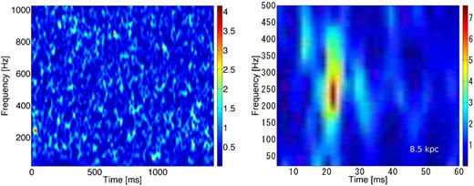
SNR of the GW from a distance of 8.5 kpc estimated in time–frequency pixels. Left: analysis based on a GW search over more than 1 s without a neutrino trigger. Right: SNR in the small time–frequency window with the aid of the neutrino timing information, corresponding to the right-hand panel of Fig. 5. Note the different scale between the left- and right-hand panels.
3.3 Electromagnetic waves
The first electromagnetic signal from a CCSN is the emission from SBO (e.g. Klein & Chevalier 1978; Falk 1978; Matzner & McKee 1999). The effective temperature of the SBO emission is estimated to be ∼4 × 10⁵ K. Thus, the emission peaks at UV wavelengths. However, as discussed below, CCSNe at the Galactic Center are likely to suffer from large interstellar extinction. Therefore, the observed spectral distribution of the SBO is likely not to peak at UV wavelengths, and observations in optical and NIR are more promising (Adams et al. 2013). For Type IIP supernovae, the SBO emission in optical and NIR wavelengths is expected to be fainter than the main plateau emission, which we discuss below, by about 1 and 2 mag, respectively (Tominaga et al. 2011).
After cooling envelope emission following SBO emission (e.g. Chevalier & Fransson 2008; Nakar & Sari 2010; Rabinak & Waxman 2011), Type IIP supernovae enter the plateau phase lasting about 100 d. The luminosity and duration of the plateau can be estimated by equations (A16)–(A17) using Mej, Ek, and R0. The solid (blue) lines in Fig. 7 show schematic light curves after the plateau phase for our s17.0 model placed at 8.5 kpc distance. The luminosity is then converted to optical (V band, 0.55 μm) and NIR (K band, 2.2 μm) magnitudes assuming a bolometric correction of Mbol–MV ≃ 0 and typical colour of MV–MK ≃ 1 (Bersten & Hamuy 2009).
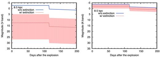
Optical (left-hand panel) and NIR (right-hand panel) signals from a Galactic CCSN at a distance of 8.5 kpc. The solid (blue) lines show schematic light curves of the plateau and tail phases based on the bolometric luminosity models given by Popov (1993) and Nadyozhin (1994). The expected light curves taking dust extinction into account are shown by dashed (red) lines with a hatched (pink) regions covering the range of half-maximum probability. The extinction correction significantly reduces the optical brightness, whereas the NIR brightness is less affected. The spatial distribution of the apparent magnitudes are shown in Fig. 8. Note that the optical and NIR magnitudes of the SBO emission are expected to be fainter than plateau magnitudes by about 1 and 2 mag, respectively (Tominaga et al. 2011).
After the plateau phase, supernovae enter the radioactive tail phase, which is powered by the decay of 56Co (daughter of 56Ni synthesized at the explosion). For the bolometric luminosity at this phase, we assume the radioactive decay luminosity with an ejected 56Ni mass of 0.028 M⊙. Then the luminosity is translated to optical and NIR magnitudes assuming Mbol–MV ≃ 0 and MV–MK ≃ 2 (Bersten & Hamuy 2009).
Despite these crude assumptions, Fig. 7 still captures the important properties of optical and NIR emissions of Galactic CCSNe. Both optical and NIR emissions are extremely bright, <−2 mag, if we do not take into account interstellar extinction (thick blue lines). However, since we have more probability to have CCSNe near the centre of the Galaxy, the observed brightness will be significantly affected by interstellar extinction.
Here, we estimate the typical range of extinction as follows, in a similar way as was done by Adams et al. (2013). First, we assume a simple 3D Galactic model both for the CCSN rate and dust distribution: |$\rho (R,Z) \propto {\rm e}^{-R/R_{\rm d}}{\rm e}^{-z/H}$|, where R is the Galactocentric radius, z is the height above the Galactic plane, and Rd and H are the scalelength and scaleheight of the Galactic disc, respectively. We adopt Rd = 2.9 kpc and H = 110 pc as in Adams et al. (2013). The Sun is placed at R = 8.5 kpc and z = 24 pc. The normalization of the dust distribution is determined such that the extinction towards the Galactic Center is AV = 30 mag.
The expected brightness maps under these assumptions are shown in Fig. 8. The optical brightness has a large diversity depending on the position (left-hand panel): it is brighter than 5 mag for nearby events while fainter than 25 mag behind the Galactic Center. On the other hand, the NIR brightness is brighter than 5 mag in almost all locations, as was also demonstrated by Adams et al. (2013). Note that Fig. 8 can also be used as the brightness distribution of the SBO emission if optical and NIR magnitudes are shifted down by about 1 and 2 mag, respectively.
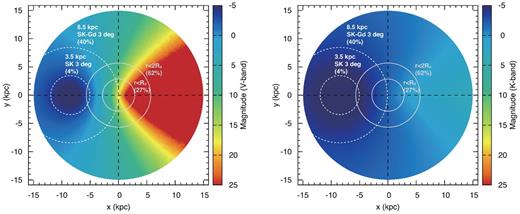
Top-down view of the Milky Way Galaxy, coloured by the expected CCSN plateau optical magnitude (left-hand panel) and NIR magnitude (right). The SBO emission is fainter by 1–2 mag than shown. The Earth is positioned at (x, y) = (−8.5, 0) kpc. The NIR magnitude is always bright enough (≲0 mag) irrespective of the location of the CCSN. On the other hand, the optical magnitude has a wide range depending on the location. Especially, the optical brightness of a CCSN at the opposite end of the Galaxy is significantly affected by dust extinction since the line of sight to the CCSN traverses more dusty regions (orange and red colours). The white dashed and grey dashed circles represent constant distances from the Earth and the Galactic Center, respectively. The circles are labelled by their radii, as well as the percentages of the Galactic CCSN rate that they contain. For circles centred on the Earth, the pointing accuracy that can be achieved by Super-K (SK) or Super-K with Gadolinium (SK-Gd) for a CCSN at the circumference is also labelled.
The expected observed light curves for CCSN events at R < Rd, which corresponds to about 27 per cent of Galactic CCSNe, are shown in Fig. 7. The dashed (red) line shows the brightness of the most probable case and the hatched region covers the range of half-maximum probability. As shown in the figure, the optical brightness is significantly affected by the extinction.
In contrast to the optical brightness, the NIR brightness is less significantly affected by extinction because extinction is much smaller in NIR, AK ∼ 0.1AV. Even in the worst case, the brightness at the plateau phase is as bright as 0–1 mag. This can be observed with the preparation of NIR telescopes/instruments usable for very bright objects (see discussions by Adams et al. 2013).
3.4 Multimessenger observing strategy
As emphasized in Adams et al. (2013), neutrinos provide crucial triggers to address important questions of IF astronomers should look for a Milky Way CCSN, WHEN they should look, and WHERE they should look. Using our CCSN model based on a long-term numerical simulation, we follow the time series of events following a core collapse. We emphasize the new insights gained when GWs are included in the discussion.
To alert the community IF one should look for a Galactic supernova, an alarm system called the SuperNova Early Warning System (SNEWS) is in place (Antonioli et al. 2004). The system consists of a network of neutrino detectors that triggers an alert when multiple detectors in different geographical locations report a burst within a certain period. The system is rapid as it does not require human intervention. The Super-K detector is large enough that a core collapse in the Milky Way will yield a high statistics neutrino burst detection (Abe et al. 2016). EGADS (Evaluating Gadolinium's Action on Detector Systems), is situated next to Super-K and is planned to be developed into a neutrino burst monitor that reports a burst within the 1-min mark while minimizing both false positives and false negatives (Vagins 2012; Adams et al. 2013).
Acquiring accurate timing information is important for improving the sensitivity for the detection of GWs. Since the coherent network analysis does not assume a priori information about a waveform, data which do not contain GWs cause degradations for detection. The accurate timing information of core bounce will thus enable one to avoid such data. The neutrinos provide timing information with 1σ uncertainties of ∼10 ms, and therefore the GW search can be started 10 ms before the time indicated by the neutrino observation (hereafter referred to as tn). The first strong amplitude of gravitational waveforms from a CCSN is known from numerous simulations to be driven by prompt-convection, and peaks within some 60 ms after core bounce (e.g. Müller et al. 2013). The GW analysis time window can therefore be set to [−10, 50] ms from tn, corresponding to a bounce time range of 0–60 ms. This procedure improves the maximal SNR of the prompt convection GW signal pixel from ∼3.5 to ∼7.5 (Fig. 6). Hence, with the coincident observation of neutrinos and GWs the detection of the GW can be claimed from the CCSN at the Galactic Center even for the case of our non-rotating progenitor.
Similarly, acquiring accurate pointing information critically impacts the feasibility of rapid electromagnetic signal follow-up (Fig. 9). As discussed above, detections in NIR wavelengths is relatively straightforward, i.e. it is almost always brighter than 5 mag. Such a bright emission can be detected with a small-aperture telescopes, whose field of views are sufficiently large in general.
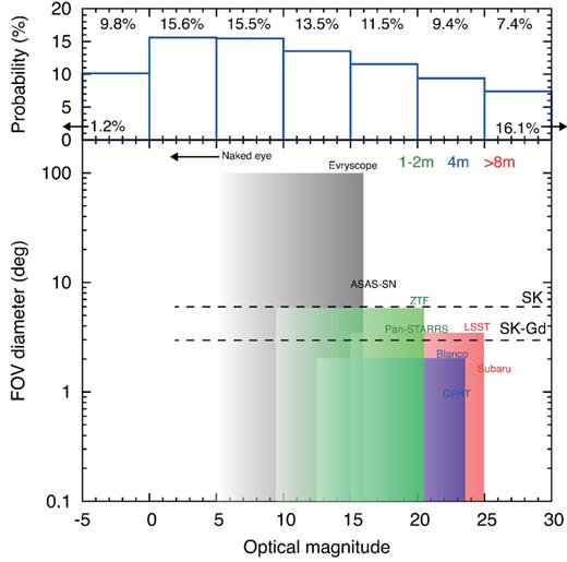
Detection prospects and strategies of the plateau signal of Galactic CCSNe. The top histogram shows the dust-attenuated plateau magnitudes with their respective percentage of the total CCSNe; 1.2 and 24.5 per cent fall beyond the magnitude range shown. The optical magnitudes of the SBO emission are also similar to the plateau magnitudes (the SBO emission is likely to be fainter by about 1 mag; Tominaga et al. 2011). The bottom panel shows the typical magnitude ranges and fields of view (FOV) of various optical telescopes: ASAS-SN, Blanco, CFHT, Evryscope, LSST, Pan-STARRS, Subaru, and ZTF (shaded rectangles), as well as the naked eye (left-pointing arrow). See the text for details. The error circle in CCSN pointing from the CCSN neutrino burst, for Super-K with and without Gadolinium, are represented by the horizontal dashed lines and labelled.
In optical wavelengths, however, the expected dust attenuation makes the early detection of the EM signals challenging. The upper panel of Fig. 9 shows the brightness distribution of the plateau emission in optical. Approximately 25 per cent of Galactic CCSNe will have apparent magnitudes >25 mag, which is difficult to observe even with the largest (8 m) optical telescopes. A further 9 per cent will be ∼20–25 mag, and require a 4–8 metre class telescope, while the dominant 40 per cent with ∼5–20 mag will require 1–2 metre class telescopes.
The SBO emission in the optical wavelength is similar to the plateau brightness (the SBO is expected to be fainter only by about 1 mag), and thus, the upper panel of Fig. 9 roughly captures the brightness distribution of the SBO emission. Since the duration of the SBO emission is only about 1 h (see Section 2.3 and Appendix A1), continuous monitoring within the error circle is critical not to miss the very first SBO signal. Therefore, the positional determination by neutrino should be good enough compared with the sizes of field of views, which depends on the apertures of telescopes.
The bottom panel of Fig. 9 shows field of views of telescopes as a function of typical magnitude limit. When the optical magnitude is brighter than ∼15 mag, the early detection is feasible thanks to the wide field of views of small-aperture telescopes. However, fainter cases are more challenging since there is no >1 m telescope with a field of view larger than ∼6° diameter (green, blue, and red regions in Fig. 9). Therefore, position determination better than 6° diameter is critical. To this end, the improved capability of a Gd-doped Super-K (SK-Gd), which enables the localization within 3° diameter for CCSNe at the Galactic Center, would be highly impactful.
Furthermore, it must be emphasized that the optical transient may follow the neutrino burst in as short as a few minutes for a collapse of a compact Wolf–Rayet star progenitor. We conclude that pre-arranged follow-up programmes will have an important role to play in securing the rise of the optical transient.
4 EXTREMELY NEARBY SUPERNOVAE
4.1 Neutrino
An extremely nearby CCSN opens new probes of the core-collapse phenomenon. An example is the detection of pre-CCSN neutrinos arising from silicon burning (Odrzywolek et al. 2004). Neutrinos are generated by nuclear processes, including beta decay and e± captures, as well as thermal processes including plasmon decay and pair annihilations (e.g. Misiaszek, Odrzywolek & Kutschera 2006; Patton & Lunardini 2015). The beta decay and pair annihilation yield O(10) MeV neutrinos, which can be detected by Hyper-K out to several kpc (Odrzywolek et al. 2004), and ≈660 pc with 1 kton KamLAND (Asakura et al. 2016). This will provide information about the pre-collapse progenitor (Kato et al. 2015) and act as an advanced warning of an imminent core collapse.
4.2 Gravitational waves
The detection of a GW from an extremely nearby CCSN is easy for advanced GW detectors such as aLIGO, adVirgo, and KAGRA. As an example, we perform simulations of the reconstruction of the GW from Betelgeuse, which is known to be in a late stage of stellar evolution and going to explode as a supernova within the next million years. The right ascension and declination of Betelgeuse is 5.9 h and 7| $_{.}^{\circ}$|4, and the distance from the Earth is 197 pc. We adopt the GW signal of our long-term simulation to be the signal from ‘Betelgeuse supernova’. In our 2D model, only the + mode of the polarization of the signal is considered. The generation of simulated data and the analysis is almost same as in Section 3.2 except that the data segment is set to 14 s, so that the signal is in one data segment for simplicity.
In the upper plot of the Fig. 10, the red and blue plots represent the injected gravitational waveform and reconstructed time series signal, respectively. The reconstructed signal is shown to be matched with the injected waveform pretty well. The middle and bottom panels show the spectrogram of the reconstructed signal in a different time-scale. To generate the spectrogram, we set the data length of the fast Fourier transform to be 20 ms. In remarkable contrast to the Galactic Center event (the right-hand panel of Fig. 5), such an extremely nearby supernova clearly presents time-evolving features. The main component at the early phase, spreading around [100–700] Hz, corresponds to the prompt-convection signal and disappears until 100 ms after bounce. Then a monotonically increasing component appears, accompanied with a subsignal around [200–300] Hz. The increasing feature is well fitted by the Brunt–|${\rm V\ddot{a}is\ddot{a}la}$| frequency at the PNS surface (Müller et al. 2013). The subsignal would be originated from some hydrodynamical instabilities like SASI (Cerdá-Durán et al. 2013).
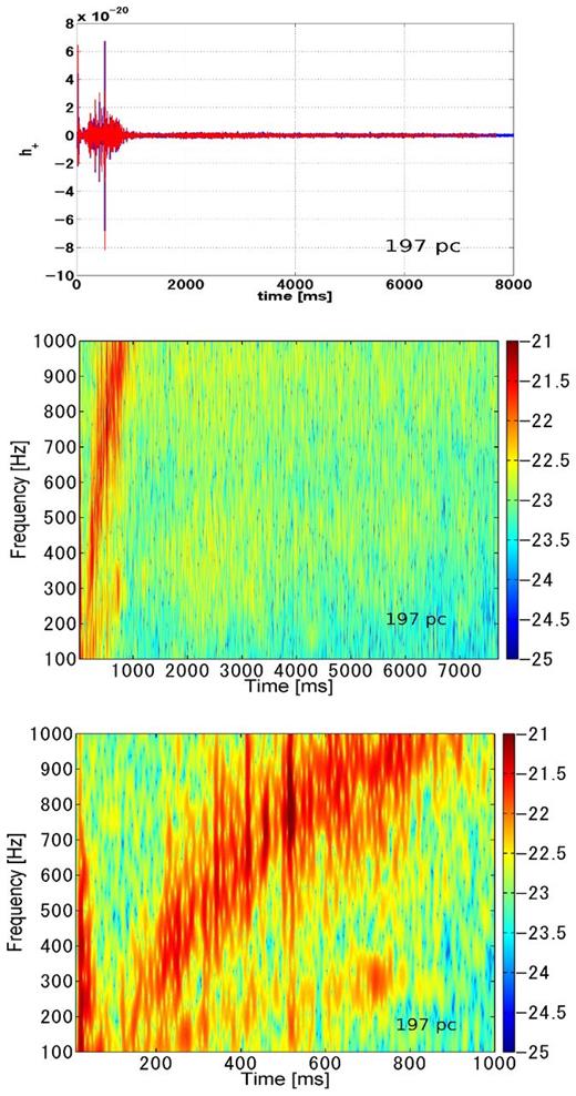
Reconstruction of the GW from Betelgeuse with the GW detector network H-L-V-K. In the top panel, the red line shows the input signal while the blue line shows time series of the reconstructed signal. The reconstruction works very well and the blue line is almost hidden behind the red line. The central and bottom panels show the spectrograms of the reconstructed signals for the first 8 and 1 s, respectively.
We inspect the detectability of these features in the same manner as in Section 3.2. The left- and right-hand panels of Fig. 11 present the SNR in time–frequency pixels of the first 1 and 8 s, respectively. In the first 1 s, the signals from the prompt-convection are clearly detectable with SNR > 100. The post-prompt-convection signals become outstanding at ∼200 ms. There are some spots with SNR 10–100 up to ∼800 ms. Thereafter, the GW energy is distributed to broad-band frequency regions and the energy of each time–frequency tile decreases. The reconstructed signals, however, still retain the time–frequency structure around 200–300 Hz up to ∼6.5 s, of which SNR is 2–5.
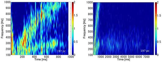
SNR of the GW from Betelgeuse for the first 1 (left-hand panel) and 8 s (right-hand panel). The colour is in logarithmic scale.
4.3 Electromagnetic waves
It is obvious that an extremely nearby CCSN within ≲1 kpc will become extremely bright both in optical and NIR wavelengths. For 1 kpc distance (distance modulus of 10 mag), the brightness of the plateau is expected to be about −6 mag. This is as bright as the recorded brightness of the Crab nebula (Stephenson & Green 2002). As is the case for SN 1054 or the Crab nebula, such CCSN explosion would be visible even in daytime. Thanks to the close distance, it is unlikely that the brightness is heavily affected by the interstellar extinction.
4.4 Multimessenger observing strategy
Extremely nearby CCSNe would provide unique information on CCSNe as well as pre-CCSN stellar evolution, and therefore, it is important not to miss any possible observables. Thanks to the pre-CCSN neutrino signal, we have a pre-CCSN alert for extremely nearby events. For CCSN neutrinos and GWs, such an alert is critical to prepare the detectors in case the detectors are not running due to, for example, maintenance works.
For electromagnetic wave signals, the pre-CCSN signal provides an unique opportunity to observe massive stars just before their collapse. Although the positional localization with pre-CCSN neutrinos is difficult, there are not too many massive stars close to the Sun, and thus, we can keep monitoring these stars after the detection of pre-CCSN neutrinos. Note that the small number of massive stars also means a low probability of CCSN rate. For example, the CCSN rate within 660 pc (detection range of 1 kton KamLAND) and 3 kpc (future Hyper-K) is about 0.1 and 4 per cent of the Galactic CCSN rate, respectively.
In Table 2, we compiled a list of nearby RSGs from the literature. RSGs associated with OB associations are taken from Levesque et al. (2005), Humphreys (1978), and Garmany & Stencel (1992), and other RSGs are supplemented from Humphreys (1970), Humphreys, Strecker & Ney (1972, table 6), White & Wing (1978), Elias, Frogel & Humphreys (1985, table 20), and Jura & Kleinmann (1990, tables 1 and 3). Note that it is difficult to distinguish RSGs and asymptotic giant branch (AGB) stars completely, since they have an overlap in luminosity (see e.g. Levesque 2010). For the purposes of listing possible CCSN progenitor candidates, we have chosen our selection to be rather inclusive. The list thus includes stars with luminosity class of II (or sometimes III), when the stars have been treated as RSG candidates in the literature, and the list may also include intermediate-mass stars. Lists of Wolf–Rayet stars, which are the progenitors of stripped envelope (H-poor) CCSNe, can be found in, e.g. van der Hucht (2001) and Rosslowe & Crowther (2015).
List of nearby RSG candidates.
| Name | RA | Dec. | Distance | V mag | Spec. type | Note | Type refa | Dist. reffb |
|---|---|---|---|---|---|---|---|---|
| (J2000.0) | (J2000.0) | (kpc) | ||||||
| BD+61 8 | 00:09:36.37 | +62:40:04.1 | 2.40 | 9.49 | M1ep Ib + B | KN Cas | 1 | 2 |
| BD+59 38 | 00:21:24.29 | +59:57:11.2 | 2.09 | 9.67 | M2 I | MZ Cas | 1 | 1 |
| HD 236446 | 00:31:25.47 | +60:15:19.6 | 2.40 | 8.71 | M0 Ib | 1 | 3 | |
| TY Cas | 00:36:59.42 | +63:08:01.7 | 2.40 | 11.5 (B) | M6 | 1 | 3 | |
| V634 Cas | 00:49:33.53 | +64:46:59.1 | 2.51 | 10.46 | M1 Iab | 1 | 3 | |
| HD 4817 | 00:51:16.38 | +61:48:19.8 | 1.05 | 6.18 | K5 Ib | HR 237 | 4 | 4 |
| HD 4842 | 00:51:26.00 | +62:55:14.9 | 2.51 | 9.62 | M6/7III | VY Cas | 1 | ** |
| BD+62 190 | 01:03:15.35 | +63:05:10.8 | 2.51 | 9.95 | M5? | 1 | ** | |
| BD+62 207 | 01:08:19.93 | +63:35:11.2 | 2.51 | 9.82 | M4 Iab | HS Cas | 1 | 2 |
| HD 236697 | 01:19:53.62 | +58:18:30.7 | 2.51 | 8.62 | M1.5 I | V466 Cas | 1 | 1 |
Notes. Only the first 10 rows are shown in this table. The full list is available in online material.
aReferences for the spectral type.
bReferences for the distance.
References:
RSGs in OB associations: (1) Levesque et al. (2005), (2) Humphreys (1978), (3) Garmany & Stencel (1992),
Other RSGs: (4) Humphreys (1970), (5) Humphreys et al. (1972), (6) White & Wing (1978), (7) Elias et al. (1985),
(8) Jura & Kleinmann (1990).
Additional references for the spectral type: * Keenan & McNeil (1989), ** classification in SIMBAD.
Our final RSG list consists of 212 RSG candidates. The typical distance limit is ∼3 kpc, which is fortunately similar to the distance limit for pre-CCSN neutrino detection with future neutrino detectors. These progenitor stars and their following electromagnetic CCSN signals are bright enough that monitoring observations soon after the pre-CCSN neutrino detection is feasible with small telescopes (Fig. 9).
5 EXTRAGALACTIC SUPERNOVAE
5.1 Neutrino
Due to its large volume, Hyper-K opens the search for neutrinos from CCSNe occurring in nearby galaxies beyond the Milky Way and Andromeda Local Group (Ando, Beacom & Yuksel 2005). Since the signal is not a statistically overwhelming burst, the detectability of the signal depends crucially on backgrounds. The main backgrounds in the O(10) MeV energy range for pure water detectors are those due to invisible (sub-Čerenkov) muons decays, atmospheric neutrinos, and spallation daughter decays (Bays et al. 2012).
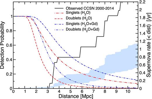
The probability of detecting at least a neutrino singlet (dot–dashed red) and at least a doublet (dashed red) from a CCSN of distance D away with Hyper-K (left axis). Positron energy bin 18–30 MeV has been assumed. The equivalents with a Gadolinium-doped Hyper-K are shown by blue lines as labelled. On the same plot, the cumulative CCSN rate within distance D is shown (right axis), estimated from observed CCSNe within the past 15 yr (solid black) and the range of estimates based on observed galaxy B-band and star formation rates (blue shaded band). The shaded band includes uncertainties arising from different indicators (B band, H α, and UV) as well as calibration factors (non-rotating and rotating stellar tracks). All estimates have been corrected for sky coverage incompleteness (see the text).
We estimate the background rate based on SK-II, which has a lower Photo-Multiplier-Tube (PMT) coverage than standard Super-K configuration and perhaps similar to the eventual Hyper-K (Abe et al. 2011). After cuts, the number of remaining backgrounds was 25 events in the signal region (here defined as 18–30 MeV energy deposited and 38–50 Čerenkov angle), for a fiducial volume of 22.5 kton and 794 d of exposure (Bays et al. 2012). This scales to a background rate of ∼286 events per 0.56 Mton year. While this is a simplified estimate ignoring differences in, e.g. signal efficiency and rock overburden, Hyper-K detector capabilities are not yet finalized, and it provides a useful starting point. The accidental coincidence rate within a 10 s window where the CCSN neutrino signal will occur is thus ∼2 × (286 yr−1)2 × (10 s) = 0.05 yr−1. In other words, two (or more) coincident events within a 10 s window would provide a compelling detection of CCSN neutrinos.
For singlet event detection, the background rate is a significant limiting factor. However, two endeavours will enhance the identification of singlet signals. The first is using the optical discovery of the CCSN as a trigger, narrowing down the time window of neutrino search. The background rate is ∼0.03 h−1, and by narrowing the time window to a few hours, the background event will be a small multiple of 0.03 (see Section 5.2 for more details). The second endeavour is background rejection due to Gadolinium doping. In pure water, the neutron left behind in IBD is captured on free protons and not registered by the detector. By doping the water with Gadolinium, the Gadolinium readily captures the neutron and produces a cascade of gamma-rays upon decay, which can be detected by the PMTs (Beacom & Vagins 2004). This way, IBD and background can be separated with high efficiency. Dominant backgrounds could be reduced by a factor ∼5, opening up the wider energy range for neutrino searches.
The occurrence rate of such opportunities is overlaid in Fig. 12, where the cumulative CCSN rate estimated directly from CCSN discoveries is shown (black solid line). We adopt the most recent 15 yr, from 2000–2014 inclusive. We start with the collection of CCSNe in the past 2000–2011 studied in Horiuchi et al. (2013), and update it with recent discoveries: SN 2012A in NGC 3239, SN 2012aw in NGC 3351, SN 2014ec in NGC 3351, and SN 2013ej in NGC 628. For all, we take distances from the 11Mpc H α and Ultraviolet Galaxy Survey (11HUGS; Kennicutt et al. 2008) catalogue of galaxies. There has been on average one CCSN per year within ∼6 Mpc. Put another way, pure water Hyper-K will have some ∼20 per cent chance of detecting neutrino doublets or greater every ∼3 yr.
The CCSN rate can also be estimated from local galaxy catalogues. For this, we adopt the CCSN estimates based on galaxy B bands and galaxy type as reported by Li et al. (2011), as well as four estimates based on galaxy star formation rate measurements: two indicators, H α and UV, each with two stellar evolutionary tracks, non-rotating and rotating. For all estimates, values were first obtained for a well-surveyed patch of sky corresponding to the survey area of the Local Volume Legacy Survey (Dale et al. 2009), then corrected for the sky that were not surveyed. The sky-coverage correction factor is 1.98 (Dale et al. 2009). Since the scatter between different estimates is larger than the formal uncertainties of each estimate, we opt to show a band which encapsulates the estimates from our five methods. Fig. 12 shows that, as pointed out previously (Ando et al. 2005; Kistler et al. 2011; Horiuchi et al. 2013), the directly estimated CCSN rate is larger than indirect estimates.
5.2 Electromagnetic waves
We do not discuss the electromagnetic wave signals from extragalactic events in detail as they are already well observed. From the multimessenger point of view, the detection of neutrinos from extragalactic events is a significant step for CCSN studies. As discussed in Section 5.1, for singlet neutrino events, we can reach several Mpc with Hyper-K. In order to firmly associate singlet neutrino detections with CCSNe, we need very early detection of electromagnetic emission, within ≲1 d after the explosion. For exceptionally well-observed CCSN, the early light curve can be used to estimate the collapse time to within a few hours (e.g. Cowen, Franckowiak & Kowalski 2010), reducing the number of single background events at neutrino detectors. In other words, electromagnetic surveys act as triggers and background reduction for neutrino searches.
For this purpose, the entire sky area should be densely monitored not to miss any CCSNe within ∼5 Mpc. Recent surveys of transients make it possible to obtain early light curves on a more regular basis. Since the absolute magnitude of the very early phase (<1 d) of CCSN is about −14 to −16 mag in optical (Tominaga et al. 2011), it will be as bright as 14.5–12.5 mag at 5 Mpc (distance modulus of 28.5 mag). This can be detected with small aperture telescopes with <1 m diameter. Ongoing projects, such as ASAS-SN (Shappee et al. 2014) and Evryscope (Law et al. 2015), will be suitable to monitor a wide area, and to detect the very early phase of very nearby CCSNe (Fig. 9). These will provide a significantly better census of CCSNe in nearby galaxies, each with very early light curves. In the following section, we discuss the observing strategy in more detail.
5.3 Multimessenger observing strategy
With only several neutrino events, the neutrino burst from an extragalactic CCSN will reveal IF to look, but it is challenging to determine WHERE to look. One method to narrow down the survey area is to use a pre-compiled list of galaxies. For this purpose, the nearby galaxy catalogue of Karachentsev et al. (2013) is the most complete. Fig. 13 shows the distribution of nearby galaxies in right ascension (the declination has been compressed). We label a few of the prominent clusters of galaxies. These structures explain the origin of sharp rise in the CCSN rate between 3 and 4 Mpc in Fig. 12. Also labelled is NGC 253, a prominent nearby star-forming galaxy.
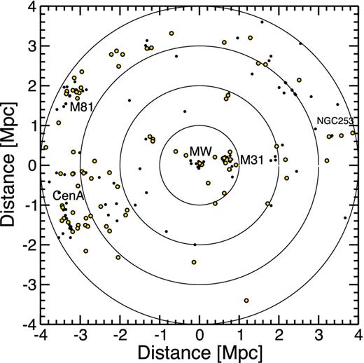
Sky plot showing the positions of nearby galaxies within 4 Mpc of the Milky Way based on the galaxy catalogue of Karachentsev et al. (2013). Clusters of galaxies in the M81 and Cen A clusters are labelled. M31, the nearest neighbouring spiral galaxy, and NGC 253, a prominent star-forming galaxy, are labelled.
The CCSN rates of the galaxies will serve as a probabilistic guide for which galaxy hosted the CCSN, which can further strategically narrow the area to survey. To estimate the CCSN rate of each galaxy, we adopt a subset of the Karachentsev catalogue for which the star formation rate can be observationally estimated. About half of the nearby galaxies have multiband observations from Spitzer-IR, H α, to GALEX-UV, providing diagnostics of the star formation rate. For example, the Karachentsev catalogue contains 236 galaxies within 5 Mpc, compared to the H α catalogue's 131 (Kennicutt et al. 2008), the UV catalogue's 154 (Gil de Paz et al. 2007), and the IR catalogue's 112 (Dale et al. 2009). Fortunately, the incompleteness is most pronounced for the least massive galaxies, and does not dramatically impact the completeness of the most important galaxies.
List of local galaxies within 5 Mpc ordered by their expected CCSN rates.
| Name | RA (°) | Dec. (°) | Dist (Mpc) | log(LH α) | Abs. B band | CCSN rate (yr−1) |
|---|---|---|---|---|---|---|
| (1) | (2) | (3) | (4) | (5) | (6) | (7) |
| NGC5236 | 204.253 | −29.866 | 4.47 | 41.25 | −20.26 | 0.024 |
| NGC253 | 011.888 | −25.288 | 3.94 | 40.99 | −20.00 | 0.013 |
| NGC3034 | 148.968 | +69.680 | 3.53 | 41.07 | −18.84 | 0.012 |
| NGC5128 | 201.365 | −43.019 | 3.66 | 40.81 | −20.47 | 0.009 |
| NGC3031 | 148.888 | +69.065 | 3.63 | 40.77 | −20.15 | 0.008 |
| Maffei2 | 040.479 | +59.604 | 3.30 | 40.76 | −20.22 | 0.008 |
| UGC2847 | 056.704 | +68.096 | 3.03 | 40.65 | −20.58 | 0.007 |
| NGC4945 | 196.365 | −49.468 | 3.60 | 40.75 | −19.26 | 0.006 |
| NGC2403 | 114.214 | +65.603 | 3.22 | 40.78 | −18.78 | 0.006 |
| NGC4449 | 187.047 | +44.093 | 4.21 | 40.71 | −18.17 | 0.005 |
Notes. Only the first 10 rows are shown in this table. The full list is available in online material.
The CCSN rates are derived from their B-band magnitudes and the LICK SNuB rates.
The galaxy catalogue is based on the compilation of Karachentsev, Makarov & Kaisina (2013).
The columns show (1) the galaxy name, (2,3) RA and declination, (4) distance,
(5) log of H α luminosity, (6) absolute B-band magnitude, (7) derived CCSN rate.
6 SUMMARY AND DISCUSSION
In this paper, we consider multimessage signals of CCSNe (in neutrinos, GWs, and electromagnetic waves) occurring at three distance regimes (the Galactic Center, a very nearby location, and extragalactic distances). Our signal predictions are self-consistently calculated based on a long-term simulation of an axisymmetric neutrino-driven core-collapse explosion (Nakamura et al. 2015) initiated from a non-rotating solar-metallicity progenitor with ZAMS mass of 17 M⊙. We consider both current and upcoming multimessenger detectors and investigate the physics reach of a future CCSN event. The detectability of multimessenger signals are summarized in Table 1, and our main findings are summarized below.
For a CCSN occurring at the Galactic Center 8.5 kpc away, the neutrino burst will be an effective trigger for subsequent multimessenger observations. The neutrino signal determines the time of core bounce to within several milliseconds. This high accuracy estimation of the bounce time allows the time window of GW analysis to be reduced, which greatly reduces the noise and makes it possible to obtain an SNR larger than that which would be possible without the neutrino trigger (Fig. 6). Secondly, the neutrino signal provides pointing information. A pure water or Gadolinium-doped Super-K will reveal the CCSN direction within an error circle of ∼6° or ∼3°, respectively. The latter is particularly important as it corresponds to the field of view of large (>1 m) modern optical telescopes (Fig. 9) which are necessary for observing the SBO emissions of CCSNe occurring at the Galactic Center and other side of the Milky Way (Fig. 8). In other words, the pointing accuracy will considerably facilitate optical follow-up.
An extremely nearby CCSN, while rare, would provide unique information of the CCSNe as well as pre-CCSN stellar evolution. The pre-CCSN neutrino signals enable us to diagnose the core structure of the CCSN progenitor and to prepare detectors for observing upcoming signals. For such an extremely nearby event, the high-precision waveform reconstruction can be done (Fig. 10, top panel) using the coherent network analysis of aLIGO, adVirgo and KAGRA. Ceaseless monitoring of nearby massive stars is essential not to miss the possible opportunities of such a rare event. To aid early follow-up, we compiled a list of nearby RSG candidates (Table 2).
At the other extreme, next-generation neutrino detectors will have sensitivity to the neutrino burst from CCSN in nearby galaxies within a few Mpc. To assist early follow-up, we compiled a list of nearby galaxies (Table 3) including their CCSN rates estimated from the H α-derived star formation rates. Within the horizon of next-generation detectors, the top 10 galaxies host more than 60 per cent of the total CCSN rate, so the number of galaxies which need follow-up is rather limited. For the GW detection, the horizon does not go beyond ∼100 kpc for our 2D (non-rotating) model even using ET (Table 1), however, it may extend to ∼Mpc distance scale if non-axisymmetric instabilities with more efficient GW emission would be captured in 3D models (Kuroda et al. 2014).
Our CCSN model is based on a 2D simulation using an approximation for neutrino transport. These numerical aspects, as well as multimessenger signal predictions, ultimately need to be investigated by using self-consistent 3D models with long-term evolution of at least ∼10 s post-bounce. Considering the rapid increase in supercomputing power (Kotake et al. 2012), we speculate that we could have access to such systematic 3D models in the not too distant future. In the near future, detectors such as KAGRA and LSST will go online, and over the next decades, advanced detectors such as DUNE, ET, and Hyper-K. Collectively, these detectors promise to deliver rich data from a future Galactic CCSN, which will be indispensable for unravelling the nature of the CCSN mechanism. Much theoretical investigations are necessary to prepare for this golden event, and our long-term 2D simulation with self-consistent multimessenger signal predictions is the first step in a string of necessary studies.
We thank John Beacom and Shoichi Yamada for valuable discussions and helpful comments. This study was supported in part by the Grants-in-Aid for the Scientific Research of Japan Society for the Promotion of Science (JSPS, Nos. 24244036, 24740117, 26707013, 26870823, and 15H02075) and the Ministry of Education, Science and Culture of Japan (MEXT, Nos. 24103005, 24103006, 25103515, 26000005, 26104001,15H00788, 15H00789, 15H01039).
Except α for νx. The leakage scheme is adopted for νx and spectrum information is not available. Here, we fix α = 2.3 for νx.
REFERENCES
SUPPORTING INFORMATION
Additional Supporting Information may be found in the online version of this article:
Table 2. List of nearby RSG candidates.
Table 3. List of local galaxies within 5 Mpc ordered by their expected CCSN rates.
Please note: Oxford University Press is not responsible for the content or functionality of any supporting materials supplied by the authors. Any queries (other than missing material) should be directed to the corresponding author for the article.
APPENDIX A: MULTIMESSENGER SIGNALS
In this appendix, we describe signals and detectors supposed in this paper.
A1 Neutrinos
For much of the post-bounce evolution, one finds a flux ordering |$F^0_{\nu _e} > F^0_{\bar{\nu }_e} > F^0_{\nu _x}$|. This ordering allows for additional flavour mixing induced by the coherent neutrino–neutrino forward scattering potential (for a review, see e.g. Duan et al. 2010; Mirizzi et al. 2016). In the inverted mass hierarchy, the observed |$F_{{\nu }_e}$| and |$F_{\bar{\nu }_e}$| are given by equations (A1)–(A2) instead of equations (A3)–(A4), but this effect is energy-dependent, giving rise to so-called spectral splits in the neutrino energy spectrum. Also, additional effects such as the ‘halo effect’ become important (Cherry et al. 2012) and exact predictions of collective flavour transformation in the post-bounce environment, and when it will apply, and at what energies, are still under debate. Therefore, the observed |$\bar{\nu }_e$| will be some mixture of |$\bar{\nu }_e$| and νx at source, whose mixture will be energy- and time-dependent. We therefore adopt equations (A1)–(A4) as two representative cases, and also consider a scenario where |$F_{{\nu }_e} = F^0_{{\nu }_e}$| and |$F_{\bar{\nu }_e} = F^0_{\bar{\nu }_e}$| (which we will call the ‘no-mixing’ scenario) to cover all extremes, as was done in Ref. (Tamborra et al. 2014).
The dominant sensitivity of Super-K and its successor Hyper-K, as well as JUNO, is to |$\bar{\nu }_e$| through the inverse beta reaction |$\bar{\nu }_e + p \rightarrow e^+ n$|. In Super-K and Hyper-K, the targets are free protons in water; for JUNO the targets are free protons in linear alkyl benzene (C6H5C12H25). The cross-section and kinematics are well known: σ(Eν) ≃ 0.0952 × 10−42(Eν − 1.3)2(1–7Eν/mp) cm2, where Eν is the neutrino energy and mp is the proton rest mass; the threshold for the reaction is Eν > 1.8 MeV; the kinetic energy of the positron Te ≃ Eν − 1.8 MeV faithfully represents the neutrino energy; and the positrons are emitted almost isotropically (Vogel & Beacom 1999; Strumia & Vissani 2003).
Elastic scattering ν + e− → ν + e− on electrons provides a strongly complementary channel to IBD. It is sensitive to all neutrino flavours, has poor neutrino energy resolution, but good angular resolution of the incoming neutrino. The recoil kinetic energy of the forward-scattered electron varies between 0 and |$2E_\nu ^2/(m_{\rm e}+2E_\nu )$|, and makes an angle |${\rm cos} \, \alpha = \sqrt{T_{\rm e}/(T_{\rm e}+2m_{\rm e})}(E_\nu +m_{\rm e})/E_\nu$|. The cross-section is also well known (Vogel & Engel 1989).
We neglect interactions with oxygen, e.g. the charge-current νe + 16O → e− + 16F* and |$\bar{\nu }_e + {\rm ^{16}O} \rightarrow e^+ + {\rm ^{16}N^{\ast }}$|, as well as all-flavour neutral-current channels (Haxton 1987). This is because they have high threshold energies and their yields are smaller compared to that from the inverse beta channel.
A2 Gravitational wave
Since |$\bf{F}$| is not a square matrix of full rank in general, the Moore–Penrose pseudo-inverse matrix |$\bf{M}:\,=\bf{F}^T\bf{F}$| is employed to obtain |$\bf{M}\boldsymbol {h}=\bf{F}^T\boldsymbol {x}$|. If the detectors are not all co-aligned, |$\bf{M}$| is an invertible m × m matrix, and we get |$\boldsymbol {h}=\bf{F}^{\dagger }\boldsymbol {x}$|, where |$\bf{F}^\dagger :\,=\bf{M}^{-1}\bf{F}^T$|.
A3 Electromagnetic waves
The first electromagnetic signal from the CCSN is the emission from SBO, which occurs when the supernova shock reaches the surface of the progenitor. Therefore, for the case of an RSG progenitor as discussed in this paper, the first electromagnetic signal will rise about 1 d after the neutrino and GW emissions. This delay enables neutrino and GW signals to be used as pre-cursors for the SBO signal. However, it should be emphasized that this delay can be as short as a few minutes for the case of Wolf–Rayet star progenitors that have significantly smaller stellar radii.
