Modelling the post-reionization neutral hydrogen (H i ) bias Free

Abstract

1 INTRODUCTION

Since its predictions by H. van der Hulst in 1944, the neutral hydrogen (H i ) 21-cm line has become a workhorse for observational cosmology. One of the direct applications of the 21-cm emission is to measure the rotation curve of galaxies (e.g. see Begum, Chengalur & Karachentsev 2005, and references therein), which is one of the most direct probes of dark matter. The 21-cm emission is also a very reliable probe of the H i content of the galaxies for the nearby Universe. Surveys like the H i Parkes All-Sky Survey (HIPASS; Zwaan et al. 2005), the H i Jodrell All-Sky Survey (HIJASS; Lang et al. 2003), the Blind Ultra-Deep H i Environmental Survey (BUDHIES; Jaffé et al. 2012) and the Arecibo Fast Legacy ALFA Survey (ALFALFA; Martin et al. 2012) aim to measure the 21-cm emission from individual galaxies at very low redshifts (z ≪1) to quantify the H i distribution in terms of the H i mass function and the H i density parameter |$\Omega _{\rm H{\scriptscriptstyle I}}$|⁠. These studies also help us in understanding the effects of different environments in which H i resides. This method fails at higher redshifts where we cannot identify individual galaxies. Here the cumulative flux of the 21-cm radiation from high-redshift emitters appears as a diffused background radiation. Measurements of the intensity fluctuations in this diffused background provide us a three-dimensional probe of the large-scale structures (LSS) over a large redshift range in the post-reionization era (z ≲ 6) (Bharadwaj, Nath & Sethi 2001; Bharadwaj & Sethi 2001; Bharadwaj & Pandey 2003; Bharadwaj & Srikant 2004). The advantage of studying the 21-cm emission in the post-reionization era lies in the fact that the modulation of the signal due to complicated ionizing fields is less and the 21-cm power spectrum is directly proportional to the matter power spectrum which enhances its usefulness as a probe of cosmology (Wyithe & Loeb 2009). This technique provides an independent estimate of various cosmological parameters (Loeb & Wyithe 2008; Bharadwaj, Sethi & Saini 2009). The Baryon Acoustic Oscillations (BAO) are embedded in the power spectrum of 21-cm intensity fluctuations at all redshifts and the comoving scale of BAO can be used as a standard ruler to constrain the evolution of the equation of state for dark energy (Chang et al. 2008; Wyithe, Loeb & Geil 2008; Seo et al. 2010).

Several existing and upcoming experiments are planned to map this radiation at various redshifts. A number of methods also have been proposed or implemented to recover the information from the signal faithfully. Lah et al. (2007a, 2009) used Giant Metrewave Radio Telescope (GMRT) observations at z ∼ 0.4 to co-add the 21-cm signals (‘stacking’) from galaxies with known redshifts in order to increase the signal-to-noise ratio and infer the average H i mass of the galaxies. This technique has been extended a little to z ∼ 0.8 by studying the cross-correlation between 21-cm intensity maps and the LSSs traced by optically selected galaxies to constrain the amplitude of the H i fluctuations (Chang et al. 2010; Masui et al. 2013). Ghosh et al. (2011a,b) devised a method to characterize and subtract the foreground contaminations in order to recover the signal and used 610 MHz (z = 1.32) GMRT observations to set an upper limit on the amplitude of the H i 21-cm signal. Kanekar, Sethi & Dwarakanath (2016) extended the signal stacking technique further to z ∼ 1.3 using GMRT observations and obtained an upper limit on the average H i 21-cm flux density.

A number of 21-cm intensity mapping experiments like Baryon Acoustic Oscillation Broadband and Broad-beam (BAOBAB; Pober et al. 2013), BAO from Integrated Neutral Gas Observations (BINGO; Battye et al. 2012), Canadian Hydrogen Intensity Mapping Experiment (CHIME; Bandura et al. 2014), the Tianlai project (Chen 2012), Square Kilometre Array 1-MID/SUR (SKA1-MID/SUR; Bull et al. 2015) have been planned to cover the intermediate-redshift range z ∼ 0.5–2.5 where their primary goal is to measure the scale of BAO, particularly around the onset of acceleration at z ∼ 1. Recent studies suggest that observations of 21-cm fluctuations on small scales, with SKA1, can constrain the sum of the neutrino masses (Villaescusa-Navarro, Bull & Viel 2015; Pal & Guha Sarkar 2016). Observations with SKA1-MID can also test different scalar field dark energy models (Hossain et al. 2016). Ali & Bharadwaj (2014) and Bharadwaj, Sarkar & Ali (2015) present theoretical estimates for intensity mapping at z ∼ 3.35 with the Ooty Wide Field Array (OWFA), while Chatterjee et al. (in preparation) and Santos et al. (2015) present similar estimates for the upcoming uGMRT and SKA2, respectively.

Several measurements of |$\Omega _{\rm H\,\small {I}}(z)$| have been carried out both at low and high redshifts. At low redshifts (z ∼ 1 and lower) we have measurements of |$\Omega _{\rm H\,\small {I}}$| from H i galaxy surveys (Zwaan et al. 2005; Martin et al. 2010; Delhaize et al. 2013), Damped Lyman α Systems (DLAs) observations (Rao, Turnshek & Nestor 2006; Meiring et al. 2011) and H i stacking (Lah et al. 2007b; Rhee et al. 2013). At high redshifts (1 < z < 6), measurements of |$\Omega _{\rm H\,\small {I}}$| come from the studies of the DLAs (Prochaska & Wolfe 2009; Noterdaeme et al. 2012). Earlier observations indicated the H i content of the Universe to remain almost constant with |$\Omega _{\rm H\,\small {I}} \sim 10^{-3}$| over the entire redshift range z < 6 (Lanzetta, Wolfe & Turnshek 1995; Storrie-Lombardi, McMahon & Irwin 1996; Rao & Turnshek 2000; Péroux et al. 2003). However, some recent studies (Sánchez-Ramírez et al. 2016) indicate that |$\Omega _{\rm H\,\small {I}}$| evolves significantly from z ∼ 2 to z ∼ 5, although the redshift evolution of |$\Omega _{\rm H\,\small {I}}$| is debatable in the intermediate-redshift range, z = 0.1–1.6 (Sánchez-Ramírez et al. 2016). A combination of low-redshift data with high-redshift observations shows that |$\Omega _{\rm H\,\small {I}}$| decreases almost by a factor of 4 between z = 5 and z = 0 (Crighton et al. 2015; Sánchez-Ramírez et al. 2016).

Martin et al. (2012) have used H i selected galaxies to estimate the H i bias b(k) at z ∼ 0.06. Intensity mapping experiments have measured the product |$\Omega _{\rm H\,\small {I}} \, b \, r$| (Chang et al. 2010; Masui et al. 2013) by studying the cross-correlation of the H i intensity with optical surveys (r here is the cross-correlation coefficient or ‘stochasticity’) while Switzer et al. (2013) have measured the combination |$\Omega _{\rm H\,\small {I}} \, b$|⁠, all these measurements being at z < 1. We do not, at present, have any observational constraint on the H i bias b(k, z) at redshifts z > 1. It is therefore important to model b(k, z) as a useful input for the future 21-cm intensity mapping experiments.

Marín et al. (2010) have developed an analytic framework for calculating the large-scale H i bias b(k, z) and studying its redshift evolution using a relation between the H i mass |$M_{\rm H\,\small {I}}$| and the halo mass M_h motivated by observations of the z = 0 H i mass function. Analytic techniques, however, are limited in incorporating the effects of non-linear clustering. In an alternative approach, Bagla, Khandai & Datta (2010) have proposed a semi-numerical technique which utilizes a prescription to populate H i in the haloes identified from dark matter only simulations. The same approach has also been used by Khandai et al. (2011) and Guha Sarkar et al. (2012) to study the H i power spectrum and the related bias. Villaescusa-Navarro et al. (2014) have used high-resolution hydrodynamical N-body simulations along with three different prescriptions for distributing the H i. Seehars et al. (2016) have proposed a semi-numerical model for simulating large maps of the H i intensity distribution at z < 1. The analytic and semi-numerical studies carried out till date are all limited in that each study is restricted to a few discrete redshifts. In a recent paper Padmanabhan et al. (2015) have compiled all the available results for the H i bias and interpolated the values to cover the redshift range z = 0–3.4. Their study is restricted to large scales where it is reasonable to consider a constant k independent bias b(z). We do not, at present, have a comprehensive study which uses a single technique to study the H i bias over a large z and k range.

In this work, we study: (i) the evolution of the H i power-spectrum |$P_{\rm H\,\small {I}}(k,z)$| across the redshift range 1 ≤ z ≤ 6 by using N-body simulations coupled with the third H i distribution model of Bagla et al. (2010), (ii) the redshift variation of the complex bias |$\tilde{b}(k,z)$| whose modulus squared, b²(k, z), relates |$P_{\rm H\,\small {I}}(k,z)$| to the matter power-spectrum P(k, z), and whose real component b_r(k, z) quantifies the cross-correlation between the H i and the total matter distribution, and (iii) the spatial (rather k) dependence of the bias and present polynomial fits which can be used to predict its variation over a large z and k range. We note that the entire analysis of this paper is restricted to real space, i.e. it does not incorporate redshift space distortion arising due to the peculiar velocities. We plan to address the effect of peculiar velocities in future. An outline of the paper follows.

In Section 2, we briefly describe the method of simulating the H i distribution. In Section 3, we present the results of our simulations. Section 3.1 contains the details of the polynomial fitting for the joint k and z dependence of the biases. The values of the fitting parameters are tabulated in Appendix. We finally summarize all the findings and discuss a few current results on the basis of our simulations in Section 4.

We use the fitting formula of Eisenstein & Hu (1999) for the ΛCDM transfer function to generate the initial matter power spectrum. The cosmological parameter values used are as given in Planck Collaboration XVI et al. (2014).

2 SIMULATING THE H i DISTRIBUTION

We follow three main steps to simulate the post-reionization H i 21-cm signal. In the first step we use a cosmological N-body code to simulate the matter distribution at the desired redshift z. Here we have used a Particle Mesh (PM) N-body code developed by Bharadwaj & Srikant (2004). This ‘gravity only’ code treats the entire matter content as dark matter and ignores the baryonic physics. The simulations use [1, 072]³ particles in a [2, 144]³ regular cubic grid of spacing 0.07 Mpc with a total simulation volume (comoving) of [150.08 Mpc]³. The simulation particles all have mass 10⁸ M_⊙ each. We have used the standard linear ΛCDM power spectrum to set the initial conditions at z = 125, and the N-body code was used to evolve the particle positions and velocities to the redshift z at which we desire to simulate the H i signal. We have considered z values in the interval Δz = 0.5 in the range z = 1 to 6.

In the next step, we employ the Friends-of-Friends (FoF) algorithm (Davis et al. 1985) to identify collapsed haloes in the particle distribution produced as output by the N-body simulations. For the FoF algorithm we have used a linking length of l_f = 0.2 in units of the mean inter-particle separation, and furthermore, we require a halo to have at least 10 particles. This sets 10⁹ M_⊙ as the minimum halo mass that is resolved by our simulation. We also verify that the mass distribution of haloes so detected are in good agreement with the theoretical halo mass function (Jenkins et al. 2001; Sheth & Tormen 2002) in the mass range 10⁹ ≤ M ≤ 10¹³ M_⊙. Our halo mass range is well in keeping with a recent study (Kim et al. 2016) which shows that at z ≥ 0.5 a dark matter halo mass resolution better than ∼10¹⁰ h⁻¹ M_⊙ is required to predict 21-cm brightness fluctuations that are well converged.

The observations of quasar (QSO) absorption spectra suggest that the diffuse Inter Galactic Medium (IGM) is highly ionized at redshifts z ≤ 6 (Becker et al. 2001; Fan, Carilli & Keating 2006a; Fan et al. 2006b). This redshift range where the hydrogen neutral fraction has a value |$x_{\rm H\,{\scriptscriptstyle I}}<10^{-4}$| is referred to as the post-reionization era. Here the bulk of the H i resides within dense clumps (column density |$N_{\rm H\,\small {I}} \ge 2\times 10^{20}{\rm cm^{-2}}$|⁠) which are seen as the DLAs found in the QSO absorption spectra (Wolfe, Gawiser & Prochaska 2005). Observations indicate that the DLAs contain almost ∼80  per cent of the total H i (Storrie-Lombardi & Wolfe 2000; Prochaska, Herbert-Fort & Wolfe 2005; Zafar et al. 2013) and they are the source of the H i 21-cm radiation in the post-reionization era. While the origin of the high-z DLAs is still not very well understood, it is found (e.g. Haehnelt, Steinmetz & Rauch 2000) that it is possible to correctly reproduce many of the observed DLAs properties if it is assumed that the DLAs are associated with galaxies. From the cross-correlation study between DLAs and Lyman Break Galaxies (LBGs) at z ∼ 3, Cooke et al. (2006) showed that the haloes with mass in the range 10⁹ < M_h < 10¹² M_⊙ can host the DLAs. In this work we assume that H i in the post-reionization era is entirely contained within dark matter haloes which also host the galaxies. In the third step of our simulation we populate the haloes identified by the FoF algorithm with H i . Here we assume that the H i mass |$M_{\rm H\,\small {I}}$| contained within a halo depends only on the halo mass M_h, independent of the environment of the halo.

We have run five statistically independent realizations of the simulation. These five independent realizations were used to estimate the mean value and the variance for all the results presented in this paper. The simulations require a large computation time, particularly the FoF which takes ∼10 d for a single realization on our computers and this restricts us to run only five independent realizations. The computation time increases at lower redshifts, and we have restricted our simulations to z ≥ 1.

As mentioned earlier, our simulations have a halo mass resolution of M_h = 10⁹M_⊙, but equation (5) shows that the mass of the smallest possible halo that retain H i falls as |$M_{\rm min} \propto (1+z)^{-\frac{3}{2}}$| and so M_min = 10⁹ M_⊙ at z = 3.5, i.e. the minimum resolvable halo mass, M_min, falls below our mass resolution of 10⁹ M_⊙ at z > 3.5. At these redshifts therefore, our simulations cannot detect haloes less massive than this threshold and which according to the model proposed by Bagla et al. (2010) are also likely to host some H i . To study the effects of these missing low-mass haloes we have run a high-resolution simulation (referred to as HRS) with [2, 144]³ particles in a [4, 288]³ regular cubic grid of spacing 0.035 Mpc, the total simulation volume remaining the same as earlier. The lower-mass limit for the halo mass is 10^8.1 M_⊙ in the HRS, well below M_min in the entire redshift range. The HRS requires considerably larger computational resources compared to the other simulations, and we have run only a single realization for which we have compared the results with those from the earlier lower resolution simulations.

3 RESULTS

Fig. 1 provides a visual impression of how the matter, the haloes and the H i are distributed at different stages of the evolution. We show this by plotting the density contrasts |$\delta ({\boldsymbol {x}},t)=\delta \rho ({\boldsymbol {x}},t)/\bar{\rho }(t)$| at three different redshifts, viz. 6, 3 and 1. It can be seen that the cosmic web is clearly visible in all three components even at the highest redshift z = 6, though it is somewhat diffused for the matter at this redshift. Observe that the basic skeleton of the cosmic web is nearly the same for all the three components, and the basic skeleton does not change significantly with redshift. We see that for all the three components the cosmic web becomes more prominent with decreasing redshift. Considering the matter first, the density contrast grows with decreasing redshifts due to gravitational clustering. The haloes are preferentially located at the matter density peaks, and it is evident that the haloes have a higher density contrast. We see that the structures in the halo distribution are more prominent compared to the matter, particularly at high redshifts. The H i closely follows the halo distribution at z = 6. However, in contrast to the matter and halo distribution, the H i distribution shows a much weaker evolution with z. It is possible to understand this in terms of the model for populating the haloes with H i. We know that the halo masses increase as gravitational clustering proceeds. According to our H i population model, however, the H i mass remains fixed once the halo mass exceeds a critical value.

Figure 1.

Shown in this figure are the matter (left panels), halo (central panels) and H i (right panels) density contrasts [|$\delta ({\boldsymbol {x}},t)=\delta \rho ({\boldsymbol {x}},t)/\bar{\rho }(t)$|], respectively, at three different redshifts 6, 3 and 1 (from top to bottom). First we calculate the over densities on the grid positions using cloud in cell (CIC) interpolation scheme. We prepare the two-dimensional density plots by collapsing a layer of thickness 5.6 Mpc along one direction to calculate the average density contrast on a plane. Different colours indicate the values of density contrast on each of the pixels as shown by the colour bar.

Open in new tabDownload slide

We quantify the matter and the H i distributions with the respective power spectra P(k) and |$P_{\rm H\,\small {I}}(k)$|⁠. We also quantify the cross-correlation between the matter and the H i through the cross-correlation power spectrum P_c(k). For all the three power spectra we consider the dimensionless quantity Δ²(k) = k³P(k)/2π², respectively, shown in the three panels of Fig. 2 for different values of the redshift z ∈ [1, 6]. The five independent realizations of the simulation each provides a statistically independent estimate of the power spectrum. We have used these to quantify the mean and the standard deviation which we show in the figures. For clarity of presentation, the ±1 σ confidence interval is shown for z = 3 only.

Figure 2.

The dimensionless form of the matter (left panel) and the H i (central panel) power spectrum, and the H i -matter cross-correlation power spectrum (right panel) are shown here as a function of k at six different redshifts. The shaded region in all three figures shows ±1 σ error around the mean value at z = 3.

Open in new tabDownload slide

The left panel of Fig. 2 shows Δ²(k) as a function of k at different redshifts. The matter distribution, whose evolution is well understood (e.g. chapter 15 of Peacock 1999) serves as the reference against which we compare the H i distribution at different stages of its evolution. It is evident that Δ²(k) increases proportional to the square of the growing mode leaving the shape of the power spectrum unchanged at small k or large length-scales where the predictions of linear theory hold (e.g. chapter 16 of Peacock 1999). At small scales, where non-linear clustering is important, the shape of Δ²(k) changes with evolution and the growth is more than what is predicted by linear theory. Note that the different power spectra shown in this paper have all been calculated using a grid whose spacing is double of that used for the simulations. The turn over seen in Δ²(k) at k ∼ 10 Mpc⁻¹ is an artefact introduced by the smoothing at this grid scale. We have restricted the entire analysis of this paper to the range k ≤ 10 Mpc⁻¹.

The central panel of Fig. 2 shows |${\Delta ^{2}_{\rm H\,\small {I}}(k)}$| as a function of k at different redshifts. We can clearly see that the evolution of Δ²(k) and |${\Delta ^{2}_{\rm H\,\small {I}}(k)}$| is quite different. At small k, we find that |${\Delta ^{2}_{\rm H\,\small {I}}(k)}$| shows almost no evolution over the entire redshift range. We find this behaviour over the entire region where the matter exhibits linear gravitational clustering. We find that |${\Delta ^{2}_{\rm H\,\small {I}}(k)}$| grows to some extent at k > 2 Mpc⁻¹ where non-linear effects are important. This growth, however, is smaller than the growth of the matter power spectrum. Further, we also see that the shape of |${\Delta ^{2}_{\rm H\,\small {I}}(k)}$| closely resembles Δ²(k) at small k; however the two differ at large k, and these differences are easily noticeable at k > 2 Mpc⁻¹.

The right panel of Fig. 2 shows |$\Delta ^{2}_{\rm c}(k)$| as a function of k at different redshifts. We see that the evolution of |$\Delta ^{2}_{\rm c}(k)$| is intermediate to that of Δ²(k) and |${\Delta ^{2}_{\rm H\,\small {I}}(k)}$|⁠; it grows faster than |${\Delta ^{2}_{\rm H\,\small {I}}(k)}$| but not as fast as Δ²(k). All three power spectra have the same shape at small k, indicating that the H i traces the matter at large length-scales. At large k the shape of |$\Delta ^{2}_{\rm c}(k)$|⁠, however, differs from both Δ²(k) and |${\Delta ^{2}_{\rm H\,\small {I}}(k),}$| indicating differences in the small-scale clustering of the H i and the matter.

The left panel of Fig. 3 shows the behaviour of b(k), the modulus of |$\tilde{b}(k)$|⁠, as a function of k at six different redshifts. We also show the 5 σ confidence interval at three different redshifts. The relatively small errors indicate that the results reported here are statistically representative values. We see that the value of b(k) decreases with decreasing redshift. Further, the k dependence is also seen to evolve with redshift. In all cases, we have a constant k independent bias at small k and the bias shoots up rapidly with k at large k (≥4 Mpc⁻¹). However, for high redshifts (z ≥ 3), b(k) increases monotonically with k whereas we see a dip in the values of b(k) at k ∼ 2 Mpc⁻¹ for z < 3. Interestingly, the k range where we have a constant k independent bias is maximum at the intermediate redshift z = 3 where it extends to k ≤ 1 Mpc⁻¹, and it is minimum (k ≤ 0.2 Mpc⁻¹) at the highest and lowest redshifts (z = 6, 1) whereas it covers k ≤ 0.4 Mpc⁻¹ at the other redshifts (z = 2, 4, 5).

Figure 3.

The left panel shows the k dependence of the H i bias b(k) at six different redshifts, z = 6 − 1 (top to bottom) at an interval Δz = 1. The shaded regions show ±5 σ error around the mean value for three redshifts 6,3 and 1. The central panel shows the k dependence of both the biases, b(k) (line only) and b_r(k) (line-point), at six different redshifts z = 6 − 1 (top to bottom) at an interval Δz = 1. For z ≥ 4, the right panel quantifies the effect of a fixed minimum halo mass which has a value M_min = 10⁹M_⊙ in the low-resolution simulations. The figure shows the fraction difference in the bias b(k) relative to a HRS.

Open in new tabDownload slide

The central panel of Fig. 3 shows both b(k) and b_r(k) which is the real part of |$\tilde{b}(k)$|⁠. The two quantities b(k) and b_r(k) show similar k dependence. Both b(k) and b_r(k) will be equal if the bias |$\tilde{b}({k})$| is a real quantity. We see that this is true at small k where both quantities have nearly constant values independent of k. However, we find a k independent bias b_r(k) for a smaller range of k, in comparison to b(k). The two quantities b(k) and b_r(k) differ at larger k, and the differences increase with increasing k. The difference between b(k) and b_r(k) is seen to increase with decreasing redshift. Also the k value where these differences become significant shifts to smaller k with decreasing redshift.

As already mentioned in Section 2, for z > 3.5, M_min (equation 4) has a value that is smaller than 10⁹ M_⊙ which is the smallest mass halo resolved by our simulations. Imposing a fixed lower halo mass limit of 10⁹ M_⊙ will, in principle, change the H i bias |$\tilde{b}(k)$| in comparison to the actual predictions of the halo population model proposed by Bagla et al. (2010), and we have run higher resolution simulation in order to quantify this. It is computationally expensive to run several realizations of simulations with a smaller mass resolution, so we have run a single realization with a halo mass resolution of 10^8.1 M_⊙ which is well below M_min over the entire redshift range of our interest. The right panel of Fig. 3 shows the percentage difference in the values of b(k) computed using the low- and the high-resolution simulations. We find that the difference is minimum for z = 4 and maximum for z = 6 where we expect a larger contribution from the smaller haloes. For k < 1.0 Mpc^{− 1}, the difference is 5–8 per cent at z = 4 and 8–13 per cent at z = 6. Beyond 1.0 Mpc^{− 1}, the difference increases but it is well within 20 per cent for redshifts 4 and 5 and less than 30 per cent for redshift 6. These differences are relatively small given our current lack of knowledge about how the H i is distributed at the redshifts of interest. It is therefore well justified to use the simulations with a fixed lower mass limit of 10⁹ M_⊙ for the entire redshift range considered in this paper.

Fig. 4 shows the redshift evolution of b(z) and b_r(z) at three representative k values. At k = 0.065 Mpc⁻¹ (left panel) which is in the linear regime we cannot make out the difference between b(z) and b_r(z) and this indicates that |$\tilde{b}(z)$| is purely real. We find that the bias b(z) has a value that is slightly less than unity at z = 1 indicating that the H i is slightly anti-biased at this redshift. The bias increases nearly linearly with z and it has a value b(z) ≈ 3 at z = 6. At k = 0.45 Mpc⁻¹ (central panel) where we have the transition from the linear to the non-linear regime we find that b(z) is slightly larger than b_r(z). Both b(z) and b_r(z) show a z dependence very similar to that in the linear regime. At k = 2.2 Mpc⁻¹ (right panel) which is in the non-linear regime we find that b_r(z) is appreciably smaller than b(z), and the difference is nearly constant over the entire z range. This indicates that the H i bias |$\tilde{b}(z)$| is complex in the non-linear regime. Further, we see that the relative contribution from the imaginary part of |$\tilde{b}(z)$| increases with decreasing z. The value of b_r(z) is less than unity for z ≤ 2, whereas this is so only in the range z ≤ 1.5 for b(z). The redshift dependence of the bias is much steeper as compared to the linear regime, and we have a larger value of b(z) ≈ 5 at z = 6. We find a nearly parabolic z dependence in the non-linear regime as compared to the approximately linear redshift dependence found at smaller k. At all the three k values we have fitted the redshift evolution of b(z) and b_r(z) with a quadratic polynomial of the form b₀ + b₁z + b₂z². We find that the polynomials give a very good fit to the redshift evolution of the simulated data (Fig. 4). We also find that the quadratic term b₂ is much larger at k = 2.2 Mpc⁻¹ as compared to the two smaller k values. Based on these results, we have carried out a joint fitting of the k and z dependence of the bias, the details of which are presented in the next section.

Figure 4.

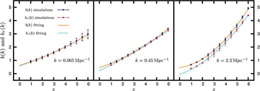
This shows the redshift evolution of b(k) and b_r(k) at three different k values. The points and the vertical error bars, respectively, show the mean and 5σ spread determined from five realizations of the simulations. The solid and dotted lines show the fitting of the respective quantities.

Open in new tabDownload slide

3.1 Fitting the bias

Figure 5.

The left panel shows the redshift evolution of the coefficients of fitting, b_m and b_rm. The square points represent the b_m values and the cross-points represent the b_rm values. The errors in fitting are enhanced five times to make them visible and shown with the vertical error bars. The solid and the dotted black lines show the best-fitting curves for b_m and b_rm, respectively. The k dependence of the simulated biases, b(k) and b_r(k), at six different redshifts z = 1−6 (bottom to top) at an interval Δz = 1, are, respectively, shown in the central and in the right panel with 5 σ error bars. The black dotted lines show the best-fitting curves.

Open in new tabDownload slide

Fig. 6 provides a visual impression of how the bias varies jointly with k and z. Here we have extrapolated our fit to cover a somewhat larger k range ([0.01, 10] Mpc⁻¹) and z range ([0, 6]). We find a scale-independent bias for k ≤ 0.1 Mpc⁻¹ across the entire z range. Further, we see that the biases b(k, z) and b_r(k, z) both decrease monotonically with decreasing z. We also see that the H i and the matter become anti-correlated where b_r has a negative value for the k range k ∼ 1–2 Mpc⁻¹ around z ∼ 0.

Figure 6.

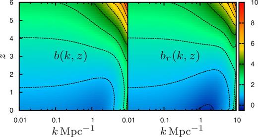
The joint k and z dependence of the biases b(k, z) (left panel) and b_r(k, z) (right panel) is shown here. The values of b(k, z) and b_r(k, z) at different points of k − z plane are represented with appropriate colours. The contours are drawn through those k and z values where the biases b(k, z) and b_r(k, z) have values in the range 0–10 (bottom to top) at an interval of 1.

Open in new tabDownload slide

The cross-correlation between the H i and the matter can also be quantified using the stochasticity (Dekel & Lahav 1999) r = b_r/b. By definition ∣r∣ ≤ 1, values r ∼ 1 indicate a strong correlation, r ∼ 0 corresponds to a situation when the two are uncorrelated and r < 0 indicates anti-correlation. Fig. 7 shows how the stochasticity r varies jointly as a function of z and k. We see that r = 1 for k ≤ 0.1 Mpc⁻¹ where the bias also is scale independent and real across the entire z range. The k value below which r is unity increases with increasing redshift, with k ∼ 0.1 Mpc⁻¹ for z = 0 and k ∼ 3 Mpc⁻¹ for z = 6. The H i and the matter are highly correlated (r > 0.8) across nearly the entire k range for z ≥ 2. We also find that r has a negative value at k ∼ 1 − 2 Mpc⁻¹ around z ∼ 0, indicative of an anti-correlation.

Figure 7.

The joint k- and z-dependence of stochasticity parameter r(k, z) ≡ b_r(k, z)/b(k, z) is shown here. The contours are drawn for the value of r = 1 to −0.5 at an interval Δr = 0.1 (left to right). The entire region to the left of the r = 1 contour corresponds to a fixed value of r = 1.

Open in new tabDownload slide

4 SUMMARY AND DISCUSSION

In this paper we have used semi-numerical simulations (the third scheme of Bagla et al. 2010) to model the H i distribution and study the evolution of |$P_{\rm H\,\small {I}}(k,z)$| in the post-reionization era. The simulations span the redshift range 1 ≤ z ≤ 6 at an interval Δz = 0.5. We have modelled the H i bias as a complex quantity |$\tilde{b}(k,z)$| whose modulus b(k, z) (squared) relates |$P_{\rm H\,\small {I}}(k,z)$| to P(k, z), and whose real part b_r(k, z) quantifies the cross-correlation between the H i and the total matter distribution. While there are several earlier works which have studied the H i bias b(k, z) at a few discrete redshifts (summarized in Padmanabhan et al. 2015), this is the first attempt to model the post-reionization H i distribution across a large z and k range (0.04 ≤ k ≤ 20 Mpc⁻¹) using a single simulation technique.

We find that the assumption of a scale-independent bias b(k, z) = b₀(z) holds at small k (equation 9). The value of b₀(z) increases nearly linearly with z, with a value that is slightly less than unity at z = 1 and b₀(z) ≈ 3 at z = 6. The k range where we have a constant k independent bias is maximum at the intermediate redshift z = 3 where it extends to k ≤ 1 Mpc⁻¹, and it is minimum (k ≤ 0.2 Mpc⁻¹) at the highest and lowest redshifts (z = 6, 1) whereas it covers k ≤ 0.4 Mpc⁻¹ at the other redshifts. The bias is scale dependent at larger k values where non-linear effects become important. We find that a polynomial fit (equation 10) provides a good description of the joint z and k dependence of b(k, z) [and also b_r(k, z)]. The coefficients of the fit are presented in Appendix, and Fig. 6 provides a comprehensive picture of the bias across the entire k and z range, all the way to z = 0 where the results have been extrapolated from the fit.

Our results which are based on a PM N-body code are qualitatively consistent with the earlier work of Bagla et al. (2010) who have used a high-resolution Tree-PM N-body code to calculate the bias at three different redshifts (z = 1.3, 3.4 and 5.1). The present work is also consistent with Guha Sarkar et al. (2012) who have used a technique similar to ours to compute the bias across z = 1.5–4, and Padmanabhan et al. (2015) who have applied the minimum variance interpolation technique to the different bias values collated from literature to predict the redshift evolution of the scale-independent bias in the range z = 0–3.4.

The analytic model of Marín et al. (2010) predicts the H i distribution to be anti-biased at low redshifts (z ≤ 1). They also found that the bias decreases further for k ≥ 0.1 Mpc⁻¹. These predictions are consistent with observations at z ∼ 0.06 (Martin et al. 2012) which suggest that H i -rich galaxies are very weakly clustered and mildly anti-biased at large scales, but become severely anti-biased on smaller scales. The predictions of our simulations which are restricted to z ≥ 1 are consistent with the findings of Marín et al. (2010). We find that the H i is mildly anti-biased at large scales at z = 1, and the bias drops further for k ≥ 0.1 Mpc⁻¹ (Fig. 3). We have also extrapolated our results to z ∼ 0 (Fig. 6) where the predictions are found to be qualitatively consistent with the measurements of Martin et al. (2012).

In our analysis the real part b_r(k, z) of the complex bias |$\tilde{b}(k,z)$| quantifies the cross-correlation between the H i and the total matter, and the bias |$\tilde{b}(k,z)$| is completely real if the two are perfectly correlated. The same issue is also quantified using the stochasticity r = b_r(k, z)/b(k, z). We see that b_r closely matches b at small k (<0.1 Mpc⁻¹) where we have a scale-independent bias across the entire z range. The complex nature of the bias becomes important at larger k. Our results are summarized in Fig. 7 which shows r across the entire z and k range. We find that the H i and the matter are well correlated (r > 0.8) across nearly the entire k range for z ≥ 2. We also find that r has a negative value at k ∼ 1 − 2 Mpc⁻¹ around z ∼ 0, indicative of an anti-correlation.

The measurements of Chang et al. (2010) constrain the product |$\Omega _{\rm H\,\small {I}} \,b \,r=(5.5 \pm 1.5) \times 10^{-4}$| at z ∼ 0.8. From our analysis, we find that on large scales the product b r ≡ b_r = 0.79 at z = 0.8 which implies |$\Omega _{\rm H\,\small {I}}=(6.96 \pm 1.89) \times 10^{-4}$|⁠. Again, Masui et al. (2013) constrain the product |$\Omega _{\rm H\,\small {I}}\, b\, r=(4.3 \pm 1.1) \times 10^{-4}$| at z ∼ 0.8 using measurements in the k range 0.05 Mpc⁻¹ < k < 0.8 Mpc⁻¹ where our work predicts br to vary from 0.83 to 0.39. The corresponding |$\Omega _{\rm H\,\small {I}}$| varies between (5.2 ± 1.3) × 10⁻⁴ and (1.1 ± 0.33) × 10⁻³, which is a significant variation. On the other hand, Switzer et al. (2013) constrain the product |$\Omega _{\rm H\,\small {I}}\, b=6.2^{+2.4}_{-1.5}\times 10^{-4}$| at z ∼ 0.8 which implies |$\Omega _{\rm H\,\small {I}}= 7.5^{+2.9}_{-1.8}\times 10^{-4}$| if we consider b = 0.83 from our analysis. The above estimates of |$\Omega _{\rm H\,\small {I}}$| are consistent with the measurement |$\Omega _{\rm H\,\small {I}}=7.41 \pm 2.71 \times 10^{-4}$| at z ∼ 0.609 (Rao et al. 2006). We note that our simulations are restricted to z ≥ 1, and the results were extrapolated to z = 0.8 for the discussion presented in this paragraph. Khandai et al. (2011) have carried out simulations which were specifically designed to interpret the results of Chang et al. (2010), and they have predicted b = 0.55–0.65 and r = 0.9–0.95 at z = 0.8. We note that the bias value predicted by Khandai et al. (2011) is considerably smaller than our prediction, and they predict |$\Omega _{\rm H\,\small {I}}=11.2 \pm 3.0 \times 10^{-4}$| which also is larger than the measurements of Rao et al. (2006).

We finally reiterate that it is important to model the H i distribution in order to correctly predict the signal for upcoming 21-cm intensity mapping experiments. Further, such modelling is also important to correctly interpret the outcome of the future observations. In the present work we have implemented a simple H i population scheme which incorporates the salient features of our present understanding, i.e. the H i resides in haloes which also host the galaxies. This, however, ignores various complicated astrophysical processes which could possibly play a role in shaping the H i distribution. Further, the entire analysis has been restricted to real space, and the effects of redshift space distortion have not been taken into account. We plan to address these issues in future work.

Debanjan Sarkar wants to thank Rajesh Mondal for his help with simulations. AS acknowledges support from the grant YSS/2014/000304 of the SERB, Department of Science & Technology, Government of India. The authors are grateful to J. S. Bagla, Nishikanta Khandai, Tapomoy Guha Sarkar and Kanan K. Datta for useful discussions.

REFERENCES

APPENDIX

The best-fitting values of the fitting coefficients c(m, n) and c_r(m, n), and the 1 σ uncertainties in fitting Δc(m, n) and Δc_r(m, n), respectively, are given below.