


Abstract
We present the effective temperatures (Teff), metallicities, and colours in Sloan Digital Sky Survey (SDSS), Two Micron All Sky Survey, and Wide-field Infrared Survey Explorer filters, of a sample of 3834 late-K and early-M dwarfs selected from the SDSS Apache Point Observatory Galactic Evolution Experiment (APOGEE) spectroscopic survey ASPCAP (APOGEE Stellar Parameters and Chemical Abundances Pipeline) catalogue. We confirm that ASPCAP Teff values between 3550 < Teff < 4200 K are accurate to ∼100 K compared to interferometric Teff values. In that same Teff range, ASPCAP metallicities are accurate to 0.18 dex between −1.0 <[M/H]<0.2. For these cool dwarfs, nearly every colour is sensitive to both Teff and metallicity. Notably, we find that g − r is not a good indicator of metallicity for near-solar metallicity early-M dwarfs. We confirm that J − KS colour is strongly dependent on metallicity, and find that W1 − W2 colour is a promising metallicity indicator. Comparison of the late-K and early-M dwarf colours, metallicities, and Teff to those from three different model grids shows reasonable agreement in r − z and J − KS colours, but poor agreement in u − g, g − r, and W1 − W2. Comparison of the metallicities of the KM dwarf sample to those from previous colour–metallicity relations reveals a lack of consensus in photometric metallicity indicators for late-K and early-M dwarfs. We also present empirical relations for Teff as a function of r − z colour combined with either [M/H] or W1 − W2 colour, and for [M/H] as a function of r − z and W1 − W2 colour. These relations yield Teff to ∼100 K and [M/H] to ∼0.18 dex precision with colours alone, for Teff in the range of 3550–4200 K and [M/H] in the range of −0.5–0.2.
1 INTRODUCTION
Late-K and M dwarfs are the most common stars in the Galaxy, dominating Galactic star counts at faint magnitudes. Because their lifetimes are longer than the age of the Universe, their numbers, compositions, positions, and motions provide a fossil record of the chemical and dynamical history of the Galaxy. Upcoming large area photometric surveys will detect an unprecedented number of these low-mass stars. It is critical to match photometric measurements of late-K and M dwarfs with their intrinsic properties so they can be used to understand Milky Way evolution. This includes, for example, an accurate and precise calibration of model isochrones so star formation histories can be correctly mapped into predicted star counts as a function of colour and apparent magnitude. The reliable fundamental properties of late-type stars are also of high importance for understanding the numerous planetary systems that have been identified around them; the mass and radius measurements for these planets are sensitive to uncertainties in the fundamental properties of their host stars.
While equations relating photometric colours with properties such as Teff, metallicity, and gravity have been determined for hotter stars in a number of filter systems (e.g. Ramírez & Meléndez 2005; González Hernández & Bonifacio 2009; Casagrande et al. 2010), such correlations have been much more difficult to produce for the coolest dwarfs. Not only are K and M dwarfs fainter than solar-type stars, but the formation of molecules in their cool atmospheres results in complex optical spectra (e.g. Valenti, Piskunov & Johns-Krull 1998) that are challenging to model accurately. Recently, fundamental parameters have been determined for some of the brightest nearby late-K and M dwarfs from a combination of high S/N, high-resolution spectroscopy and interferometry (Casagrande, Flynn & Bessell 2008; Boyajian et al. 2012; Rajpurohit et al. 2013). These parameters are not immediately useful for calibration, however, because they are frequently above the saturation limit for good survey photometry.
The most comprehensive relationships between photometry and fundamental properties have instead been based on low-resolution spectroscopy. Mann et al. (2015) used low-resolution infrared spectra to derive colour–Teff relations for K7–M7 stars using spectrophotometrically derived VRCICgrizJHKs and Gaia filters as part of their comprehensive work on bolometric corrections, radii, and masses for such stars. Newton et al. (2014) also used low-resolution infrared spectroscopy to derive a photometric metallicity relation for M0–M7 using filters from the Two Micron All Sky Survey (2MASS; Skrutskie et al. 2006). The relationship between colour and metallicity in Sloan Digital Sky Survey (SDSS) ugriz filters was most recently examined by Bochanski et al. (2013), using metal-poor subdwarfs identified in SDSS low-resolution spectroscopy (Savcheva, West & Bochanski 2014).
Therefore, the colours of cool dwarfs with measured Teff and metallicity have not yet been determined observationally for the ugriz filters and the mid-infrared filters recently used by the Wide-field Infrared Survey Explorer (WISE; Wright et al. 2010). Determining the association between the observed SDSS colours, including the u-band, and fundamental properties of late-type stars is key to studying the stellar populations of SDSS, which, because of its relatively deep photometry and large sky coverage off of the Galactic plane, is a rich source of M dwarfs (e.g. Jurić et al. 2008; Bochanski et al. 2010).
The high-resolution near-IR spectra of the Sloan Digital Sky Survey III (SDSS-III; Eisenstein et al. 2011; Ahn et al. 2014) Apache Point Observatory Galactic Evolution Experiment (APOGEE; Majewski et al. 2015) observed late-type stars in ∼650 fields. Each of these stars has photometry from 2MASS and WISE, and a subset of APOGEE stars were both located in the SDSS photometric footprint and faint enough that their SDSS ugriz photometry is not saturated. We explore a limited range of late-K and early-M dwarfs with both APOGEE observations and high quality SDSS-2MASS-WISE photometry to relate the fundamental properties (Teff and [M/H]) predicted by stellar population modelling with colours. This combination of colours and fundamental properties also provides important tests of current stellar isochrones.
In Section 2, we describe the selection of our late-K and early-M (hereafter KM) dwarf sample and verify the Teff and [M/H] from the APOGEE catalogue. Section 3 discusses the SDSS, 2MASS, and WISE photometry and Section 4 describes the model grids we use for comparison. In Section 5 we examine the relationships between colours, Teff, and [M/H] in both the models and the data and provide empirical relationships between Teff, [M/H] and colour.
2 APOGEE SPECTROSCOPY
The APOGEE survey (Majewski et al. 2015), part of SDSS-III (Eisenstein et al. 2011; Ahn et al. 2014), uses a multi-object near-infrared spectrograph (Wilson et al. 2010) operating on the 2.5-m Sloan Foundation Telescope (Gunn et al. 2006) at Apache Point Observatory. The spectra cover most of the H-band from 1.51–1.70 μm with an average resolution of R∼22 500. The targets were generally selected based on 2MASS J − Ks dereddened colours and an H-band magnitude limit extending down to 13.8 mag, although most fields have H ≤ 12.2 mag (see Zasowski et al. 2013, for a description of the target selection). Additional stars were specifically targeted for survey calibration. For the brightest stars, spectra were obtained by running a fibre from the NMSU 1-m to the APOGEE instrument and observing when the APOGEE instrument was not taking data at the 2.5-m telescope (Holtzman et al. 2015). These brighter stars were selected due to previously well-determined properties, and include both Gaia benchmark stars (Jofré et al. 2014) and stars with interferometric radii (Boyajian et al. 2012). As of SDSS-III Data Release 12 (DR12; Alam et al. 2015), APOGEE obtained 618 080 spectra of 156 593 stars, primarily red giants used to trace Galactic structure. In general, the M dwarfs observed by APOGEE fell serendipitously into the normal APOGEE colour and magnitude cuts as red stars, were targeted as SEGUE overlap targets, or were targeted as part of the M-dwarf ancillary project (Deshpande et al. 2013).
2.1 APOGEE spectroscopic parameters
Stellar parameters were measured from the H-band spectra by the APOGEE Stellar Parameters and Chemical Abundances Pipeline (ASPCAP; García Pérez et al. 2015), which determines the χ2 minima between the observed spectra and a six-dimensional grid of synthetic spectra (Zamora et al. 2015). The six dimensions varied are Teff, log g, [M/H], [C/M], [N/M], and [α/M] (for additional detail see Zamora et al. 2015). The ranges spanned by the grid in DR12 are 3500–8000 K in Teff, 0–5 dex in log g, −2.5 to 0.5 dex in [M/H], and −1 to 1 for [C/M], [N/M], and [α/M]. The cool temperature edge is of particular concern for this work, as it limits our current effort to early-M and warmer (KM) dwarfs. ASPCAP parameters become increasingly unreliable as the grid edge is approached; requiring reliable Teff measurements essentially restricts our sample to stars with Teff ≥ 3550K.
In the ASPCAP minimization, the [M/H] axis varies the abundances of all elements relative to the solar values. However, the [α/M] axis independently varies the abundances of α elements (O, Mg, Si, S, Ca, Ti). Therefore, the [M/H] reported by ASPCAP is sensitive mainly to the lines of iron-peak elements and maps well on to [Fe/H] values in the literature (Mészáros et al. 2013; Holtzman et al. 2015).
Holtzman et al. (2015) performs an extensive comparison of ASPCAP parameters for red giants with photometric Teff, seismic log g values, and literature metallicities for cluster stars. Due to the existence of these comparison values, the ASPCAP parameters for giants are calibrated to better match previous data. The ASPCAP values for dwarf stars were also examined, revealing systematically low log (g) values compared to isochrone predictions and difficulties properly treating rotation in the model grid. In Sections 2.3 and 2.4, we compare the uncalibrated ASPCAP values for KM dwarfs to literature values to assess the reliability of ASPCAP parameters for studying the colours of these stars in additional filter sets.
2.2 Selecting KM dwarfs from APOGEE DR12
From the DR12 APOGEE catalogue, we selected stars with effective temperatures of 3500 K ≤Teff ≤ 4200 K and log (g) ≥ 4.0. These stars overlap with spectral types K5–M2 (Boyajian et al. 2012; Pecaut & Mamajek 2013) and form the low temperature, low-gravity edge of the ASPCAP grid; while there are cooler APOGEE targets, the DR12 release does not include their properties. We selected the best observations of stars that were targeted on multiple plates by excluding those with the EXTRATARG flag set to 4.
Our initial sample included 7784 stars, but we excluded 1139 spectra targeted as part of an ancillary programme to examine embedded young cluster stars as those stars have peculiar colours. We then performed flag cuts to ensure the quality of the catalogue parameters for the 6604 remaining stars. We excluded stars with Teff and [M/H] flagged as bad, typically due to the proximity of a value to the edge of the model grid (most notably the lower Teff boundary). We also excluded stars flagged for low S/N (corresponding to S/N per pixel <70), a warning or bad flag set due to possible rapid rotation, and high χ2 values (warn or bad). The sample of stars with reliable ASPCAP parameters includes 4246 stars; those with reliable extinction corrections (see Section 3.4) are listed in Table 1.1
Properties of APOGEE KM dwarfs. This table is a shortened version provided as a guide. Complete table available online.
| 2MASS ID | ASPCAP | SDSS | 2MASS | WISE | APASS | V − Ja | |$V-K_S^{b}$| | ||||||||
|---|---|---|---|---|---|---|---|---|---|---|---|---|---|---|---|
| 2MASS J | Teff (K) | [M/H] | u | g | r | i | z | J | H | KS | W1 | W2 | V | Teff (K) | Teff (K) |
| 00012151+5634379 | 3934 | 0.06 | – | – | – | – | – | 10.43 ± 0.02 | 9.72 ± 0.03 | 9.52 ± 0.02 | 9.45 ± 0.02 | 9.48 ± 0.02 | 13.41 | 3812 | 3768 |
| 00012252+1558339 | 3775 | −0.18 | 19.31 ± 0.03 | 16.72 ± 0.02 | 15.29 ± 0.02 | 14.45 ± 0.01 | 13.98 ± 0.02 | 12.76 ± 0.02 | 12.09 ± 0.03 | 11.92 ± 0.02 | – | 11.71 ± 0.02 | – | – | – |
| 00012694+1639052 | 3712 | −0.51 | 18.80 ± 0.03 | – | 15.04 ± 0.02 | – | 13.71 ± 0.02 | 12.51 ± 0.02 | – | – | 11.61 ± 0.02 | 11.51 ± 0.02 | 15.58 | 3657 | – |
| 00013219+0016012 | 4012 | −0.42 | – | 15.60 ± 0.01 | – | – | 13.44 ± 0.01 | – | 11.62 ± 0.02 | 11.52 ± 0.02 | 11.39 ± 0.02 | 11.40 ± 0.02 | 14.90 | – | 3939 |
| 00013817+0017293 | 3671 | −0.19 | 18.84 ± 0.03 | 16.32 ± 0.02 | 14.97 ± 0.02 | – | 13.28 ± 0.01 | 12.01 ± 0.02 | 11.33 ± 0.02 | 11.10 ± 0.02 | 11.01 ± 0.02 | 10.94 ± 0.02 | 15.62 | 3476 | 3423 |
| 00015592+0027057 | 4046 | −0.11 | 18.99 ± 0.03 | 16.38 ± 0.01 | – | 14.44 ± 0.01 | 14.09 ± 0.01 | 12.93 ± 0.02 | 12.23 ± 0.02 | 12.09 ± 0.02 | 12.02 ± 0.02 | 12.05 ± 0.02 | 15.72 | 3889 | 3850 |
| 00015966+1627449 | 4132 | −0.12 | – | – | – | – | – | 10.73 ± 0.02 | – | – | 9.79 ± 0.02 | 9.85 ± 0.02 | 13.23 | 4080 | – |
| 00022557+0126203 | 4068 | 0.06 | 19.45 ± 0.03 | 16.73 ± 0.02 | 15.38 ± 0.01 | 14.68 ± 0.02 | 14.30 ± 0.02 | – | 12.50 ± 0.02 | 12.32 ± 0.02 | – | 12.25 ± 0.02 | 15.85 | – | 3953 |
| 00023747−0010572 | 3882 | −0.32 | 19.77 ± 0.03 | 17.12 ± 0.02 | 15.72 ± 0.01 | 15.00 ± 0.02 | 14.66 ± 0.02 | 13.40 ± 0.02 | 12.73 ± 0.02 | 12.57 ± 0.02 | – | – | – | – | – |
| 00025988+0148410 | 4053 | −0.28 | 18.98 ± 0.03 | 16.34 ± 0.03 | – | – | – | 12.90 ± 0.02 | 12.29 ± 0.02 | – | 12.03 ± 0.02 | 12.03 ± 0.02 | 15.51 | 3975 | – |
| 00030930+0110025 | 3996 | −0.36 | 19.23 ± 0.03 | 16.65 ± 0.02 | 15.32 ± 0.01 | 14.75 ± 0.01 | 14.44 ± 0.01 | 13.25 ± 0.02 | 12.61 ± 0.03 | 12.43 ± 0.02 | 12.36 ± 0.02 | – | – | – | – |
| 00031412+0037379 | 3930 | 0.04 | 19.10 ± 0.03 | 16.42 ± 0.02 | – | 14.60 ± 0.01 | 14.29 ± 0.02 | – | – | 12.34 ± 0.02 | – | 12.27 ± 0.02 | 15.70 | – | 4045 |
| 00031777+1636147 | 3909 | −0.36 | 18.84 ± 0.03 | – | 14.95 ± 0.01 | 14.28 ± 0.01 | 13.86 ± 0.01 | 12.68 ± 0.02 | – | 11.86 ± 0.02 | – | 11.75 ± 0.02 | 15.54 | 3801 | 3764 |
| 00033020+0020078 | 3964 | −0.10 | 19.55 ± 0.03 | 16.89 ± 0.02 | – | – | 14.53 ± 0.02 | 13.33 ± 0.02 | 12.69 ± 0.03 | 12.44 ± 0.02 | 12.41 ± 0.02 | 12.45 ± 0.02 | – | – | – |
| 00033817+0020226 | 3907 | −0.18 | 19.14 ± 0.02 | 16.49 ± 0.02 | – | – | 14.00 ± 0.02 | 12.81 ± 0.02 | 12.13 ± 0.03 | 11.94 ± 0.02 | 11.86 ± 0.02 | 11.85 ± 0.02 | 15.78 | 3772 | 3717 |
| 00035823+7351001 | 4114 | −0.17 | – | – | – | – | – | – | – | 11.96 ± 0.02 | – | 11.87 ± 0.02 | 16.08 | – | 3586 |
| 00035968+1542051 | 3924 | −0.26 | 18.86 ± 0.03 | 16.34 ± 0.02 | – | 14.34 ± 0.02 | 13.99 ± 0.02 | 12.78 ± 0.02 | 12.09 ± 0.03 | 11.99 ± 0.02 | 11.92 ± 0.02 | 11.91 ± 0.02 | 15.62 | 3830 | 3809 |
| 00041959+7547098 | 3545 | −0.30 | – | – | – | – | – | 12.11 ± 0.02 | 11.54 ± 0.03 | 11.30 ± 0.02 | 11.15 ± 0.02 | 11.00 ± 0.02 | – | – | – |
| 00042083+0158446 | 4133 | −0.23 | – | – | – | – | – | – | 11.96 ± 0.03 | 11.78 ± 0.02 | 11.70 ± 0.02 | 11.73 ± 0.02 | 15.08 | – | 4026 |
| 00043956+1525247 | 3550 | −0.29 | 18.16 ± 0.02 | 15.72 ± 0.01 | – | – | 12.64 ± 0.02 | 11.30 ± 0.02 | 10.77 ± 0.03 | 10.51 ± 0.02 | 10.39 ± 0.02 | 10.31 ± 0.02 | 14.98 | 3432 | 3410 |
| 00044424+0038241 | 3786 | −0.04 | 19.41 ± 0.03 | 16.84 ± 0.02 | 15.46 ± 0.01 | 14.78 ± 0.02 | 14.41 ± 0.02 | 13.23 ± 0.02 | 12.59 ± 0.02 | 12.36 ± 0.02 | – | – | – | – | – |
| 00044471−0011336 | 4022 | −0.13 | 18.56 ± 0.02 | 15.90 ± 0.02 | – | – | 13.49 ± 0.01 | 12.33 ± 0.02 | 11.63 ± 0.03 | 11.48 ± 0.02 | 11.39 ± 0.02 | 11.42 ± 0.02 | 15.10 | 3901 | 3849 |
| 00044671+0125326 | 4005 | −0.27 | – | – | – | – | – | 12.93 ± 0.02 | 12.27 ± 0.02 | 12.10 ± 0.02 | – | 12.00 ± 0.02 | 15.52 | 3985 | 3942 |
| 00044884-0032341 | 4073 | −0.29 | – | 16.49 ± 0.02 | 15.16 ± 0.02 | 14.58 ± 0.02 | 14.26 ± 0.01 | 13.13 ± 0.02 | 12.48 ± 0.03 | – | – | 12.22 ± 0.02 | 15.71 | 3993 | – |
| 00054076+0001181 | 4024 | −0.37 | 18.33 ± 0.02 | 15.73 ± 0.01 | – | – | 13.45 ± 0.02 | 12.25 ± 0.02 | 11.60 ± 0.02 | 11.45 ± 0.02 | – | 11.37 ± 0.02 | 14.96 | 3897 | 3873 |
| 00054249+0022537 | 4003 | −0.25 | 19.34 ± 0.03 | 16.78 ± 0.02 | 15.45 ± 0.02 | – | 14.49 ± 0.02 | – | 12.64 ± 0.02 | 12.48 ± 0.02 | 12.45 ± 0.02 | – | – | – | – |
| 00055969−0030062 | 4027 | −0.38 | 19.15 ± 0.03 | 16.51 ± 0.03 | 15.15 ± 0.02 | 14.60 ± 0.01 | – | 13.10 ± 0.02 | 12.45 ± 0.02 | 12.28 ± 0.02 | – | 12.19 ± 0.02 | – | – | – |
| 00060369+0104479 | 4105 | −0.48 | – | – | – | – | – | 12.90 ± 0.02 | 12.23 ± 0.03 | 12.05 ± 0.02 | 11.98 ± 0.02 | 12.00 ± 0.02 | – | – | – |
| 00060971+0120321 | 3745 | 0.09 | – | – | – | – | – | – | 12.67 ± 0.03 | – | 12.32 ± 0.02 | – | – | – | – |
| 00061237+0101599 | 3968 | −0.16 | 19.29 ± 0.03 | 16.68 ± 0.02 | 15.29 ± 0.02 | 14.61 ± 0.01 | 14.21 ± 0.01 | 13.03 ± 0.02 | 12.32 ± 0.03 | – | 12.07 ± 0.02 | 12.07 ± 0.02 | 15.80 | 3893 | – |
2.3 Accuracy of effective temperature
We determined the accuracy of the ASPCAP Teff values by comparing them to previously determined Teff values derived from multiple sources, as shown in Fig. 1. The most accurate and precise Teff values are determined using a combination interferometric radii and bolometric luminosities. Five stars in the APOGEE KM sample (and one additional star with an ASPCAP Teff = 4215 K) have interferometric Teff measurements from Boyajian et al. (2013); these stars are listed in Table 2, and their comparison is shown in the top panel of Fig. 1. The ASPCAP Teff values are 130 K hotter than the interferometric Teff values, with an rms scatter of 30 K. The comparison between these six values and the ASPCAP values reveals no systematic dependence on [M/H] or Teff, but the sample size is too small to rule out systematic issues.
![ASPCAP Teff compared to Teff from multiple literature sources. In the top panel, the Boyajian et al. (2013) interferometric (large grey circles) and V − K (small coloured circles) Teff. In the middle panel, the (Mann et al. 2015) colour–Teff using V − J colour combined with ASPCAP [M/H] values (see their equation 6). The bottom panel, the (Casagrande et al. 2008) infrared flux technique Teff. In every panel, the points are colour coded by ASPCAP [M/H] values and a one-to-one correspondence line is shown.](https://oup.silverchair-cdn.com/oup/backfile/Content_public/Journal/mnras/460/3/10.1093_mnras_stw1139/2/m_stw1139fig1.jpeg?Expires=1750588206&Signature=lhtmfhs2B1YGaRnFyOH3aYwQJErmeexnI7ytDpl54S1yz5F65Hvdd4Lv1KOCLQ~uXw7EPe8~Xx40KBJjbwJSz8pahpCMQ0QWOWwZhTiPbqjPKy-oDoMx8PnHaZC0LkRHSxPMn7IaXUONNWGRakfC8E03-WBpglD1bZqMYIzpMG7HutEvAAWcAfNd7ny7I9YxXNdE1JdVOAd~d7FCZYbGYjgCLsMdHMB95FHxAmbC4izUqN4nI5NKiwv42JYTHBEccvKLp5W11tdut-NGlk32S6fcyt21FFFPl24mzkytsxFlFH6InLNF1N5lutc8AuoMSKpFnj26zkc1DLUfotjoLA__&Key-Pair-Id=APKAIE5G5CRDK6RD3PGA)
ASPCAP Teff compared to Teff from multiple literature sources. In the top panel, the Boyajian et al. (2013) interferometric (large grey circles) and V − K (small coloured circles) Teff. In the middle panel, the (Mann et al. 2015) colour–Teff using V − J colour combined with ASPCAP [M/H] values (see their equation 6). The bottom panel, the (Casagrande et al. 2008) infrared flux technique Teff. In every panel, the points are colour coded by ASPCAP [M/H] values and a one-to-one correspondence line is shown.
Comparison of ASPCAP Teff with Teff from interferometric radii.
| 2MASS ID | Other | Interfer.a | ASPCAP | |
|---|---|---|---|---|
| name | Teff (K) | Teff (K) | [M/H] | |
| 05312734−0340356 | GJ205 | 3801 ± 9 | 3871 | 0.16 |
| 09142298+5241125 | GJ338A | 3907 ± 35 | 4069 | −0.12 |
| 10112218+4927153 | GJ380 | 4081 ± 15 | 4215 | 0.02 |
| 11032023+3558117 | GJ411 | 3465 ± 17 | 3588 | −0.71 |
| 11052903+4331357 | GJ412A | 3497 ± 39 | 3670 | −0.60 |
| 17362594+6820220 | GJ687 | 3413 ± 28 | 3543 | −0.08 |
aFrom Boyajian et al. (2013).
In addition to providing individual measurements, Boyajian et al. (2013) also used interferometric radii and bolometric luminosities to calibrate a V − K/Teff relation. We combined V-band photometry for 2446 APOGEE stars in our sample from the AAVSO Photometric All Sky Survey (APASS; Henden & Munari 2014) Data Release 8 (corrected for extinction as described in Section 3.4) with 2MASS KS magnitudes (see Section 3) to derive photometric Teff values based on that relation; the comparison is shown in the top panel of Fig. 1 and the V magnitudes and calculated Teff values are included in Table 1. The formal uncertainties on the V − KTeff values are small (∼30 K) due to low photometric uncertainties (0.02–0.03 mag) and a small scatter in the relation (2 per cent; Boyajian et al. 2013). Overall, the ASPCAP Teff values are 130 K hotter than the photometric Teff values, with an rms scatter of 81 K. There is no evidence of a metallicity dependence in the comparison between the two sets of values.
Mann et al. (2015) derived colour–Teff relations for M dwarf using the method described by Mann, Gaidos & Ansdell (2013b) that relies on the comparison of low-resolution infrared spectra to the BT-Settl version of the phoenix atmosphere models (Allard et al. 2003). We compared the ASPCAP Teff values to those calculated from the Mann et al. (2015) relation as a function of V − J colour that includes an explicit [M/H] term (shown in the middle panel of Fig. 1 and included in Table 1). The ASPCAP values are 101 K hotter with an rms scatter of 79 K2 The offset and scatter are similar to the Boyajian et al. (2013) offset because the Mann et al. (2013b) method for determining Teff values was explicitly tuned to best match the Boyajian et al. (2013) relations.
Casagrande et al. (2008) calculate Teff values based on the infrared flux technique and derive a relationship based on V − K colour. The bottom panel of Fig. 1 shows these Teff values compared to ASPCAP Teff values. The mean agreement is poor; the ASPCAP values are 161 K warmer than those from the V − K/Teff relation and have a scatter of 140 K. The lack of agreement stems primarily from the absence of [M/H] from the Teff calculation; higher metallicity stars ([M/H]∼0) have ASPCAP Teff values that are 200–300 K hotter their V − KTeff values, while lower metallicity stars ([M/H]∼− 0.6) fall closer to the 1:1 line.
Based on these comparisons, it is clear that there is a metallicity dependence that must be taken into account to calculate accurate Teff values using photometry. From the comparison with the Boyajian et al. (2013) values, it is likely that the ASPCAP Teff values for KM dwarfs are overestimated by ∼130 K. We discuss the effect of this offset as part of Section 5.
We used 25 APOGEE KM stars with duplicate observations that pass our quality cuts as an additional check on the uncertainty. The duplicate observations were on average 22 K warmer with a dispersion of 74 K. We adopt an overall Teff uncertainty of 100 K based on both the duplicate observations and the scatter in the comparison between the APOGEE KM values and those from both Boyajian et al. (2013) and Mann et al. (2015).
2.4 Accuracy of metallicities
To test the accuracy of the ASPCAP [M/H] values, we compared them to measurements of the metallicities of M dwarfs derived from either high-resolution spectroscopic analysis of individual M dwarfs or of hotter primaries in binary systems with a secondary M dwarf. Table 3 includes these values and Fig. 2 shows the comparison. The ASPCAP metallicities are consistent with previous analysis; on average they are 0.07 dex more metal rich with a scatter of 0.18 dex. Uncertainties listed for these values in the literature do not always take into account systematic uncertainties in the abundance analysis, which can be important when combining a heterogeneous set of metallicity derivations as is done here. However, comparison of metallicities for well-studied stars in the literature, in particular for the Gaia benchmark stars (Jofré et al. 2014) show that the scatter there is typically <0.1 dex. Both of these effects are larger than the differences between the 25 high-quality duplicate observations, which have difference of [M/H] = 0.007 and a scatter of 0.035 dex. Therefore, we conservatively adopt 0.18 as the uncertainty in the ASPCAP metallicities and hope to be able to compare to a large set of homogeneously derived high-resolution analyses in the future. For reference, we also show in Fig. 2 the comparison of our values to literature values that are derived from low-resolution spectral indices calibrated to higher dispersion measurements.
![ASPCAP [M/H] values compared to literature [Fe/H] values for high-resolution literature sample (filled circle colour coded by Teff). We also show the comparison for stars we have in common with the measurements based on the calibration of low-resolution spectra from Terrien et al. (2015), Newton et al. (2014), and Muirhead et al. (2012). The overall comparison with other high-resolution analyses is good.](https://oup.silverchair-cdn.com/oup/backfile/Content_public/Journal/mnras/460/3/10.1093_mnras_stw1139/2/m_stw1139fig2.jpeg?Expires=1750588206&Signature=n0X~~Jj2jLpPjFu96BI8fBIzbdXnOPRoWnhz2xOmrAb7pDRkjEs5eyG0E6vRYFezHnSJhgQhxqvku-WJi8-eU9vP83rvuP3njFSGr-KVzJUQMxXYN7qjTK5B401eNnCi34W-xhnzckaa2qAhmHcPs9UfClBFpOaDqeM-nkKSlQ9mMGaHnt2xc1ZonIJiFy3JtPxr7rFHE9W2wsFoM8HmzUsTe7y~pWW6g26f5s2IWBzeHj8S-u~xqCLNcqvCoMDiXpZkbF~cpYvENJ0kCDAMCYBiplv2tmkeN3nllC1l06vy5UqMG8cK~lOBfdO807baWmGJFyRo2-GX2sfwWyX25w__&Key-Pair-Id=APKAIE5G5CRDK6RD3PGA)
ASPCAP [M/H] values compared to literature [Fe/H] values for high-resolution literature sample (filled circle colour coded by Teff). We also show the comparison for stars we have in common with the measurements based on the calibration of low-resolution spectra from Terrien et al. (2015), Newton et al. (2014), and Muirhead et al. (2012). The overall comparison with other high-resolution analyses is good.
Comparison with literature metallicities.
| 2MASS ID | Other ID | ASPCAP [M/H] | Literature [Fe/H] | Lit. method | Reference |
|---|---|---|---|---|---|
| 2M01081597+5455148a | muCas | −0.82 | −0.81 | High-res | 1 |
| 2M02043481+1249453 | −0.54 | −0.41 | Low-res | 2 | |
| 2M02410716+5423087 | 0.035 | 0.61 | Low-res | 2 | |
| 2M03150093+0103083 | NLTT10349 | −0.98 | −0.92 | Binary | 3 |
| 2M03285302+3722579 | LHS173 | −0.94 | −1.19 | High-res | 4 |
| 2M04342248+4302148 | −0.09 | 0.22 | Low-res | 2 | |
| 2M05011802+2237015 | −0.91 | 0.24 | Low-res | 2 | |
| 2M05312734−0340356 | GJ205 | 0.16 | 0.21 | High-res | 4 |
| 0.16 | 0.35 | Low-res | 5 | ||
| 2M05454158+1107485 | 0.04 | 0.30 | Low-res | 2 | |
| 2M06181761+3200593 | −0.07 | 0.02 | Low-res | 2 | |
| 2M06312373+0036445 | NLTT16628 | −0.50 | −0.54 | Binary | 3 |
| 2M06561894−0835461 | −0.57 | 0.10 | Low-res | 2 | |
| 2M08103429−1348514 | GJ297.2B | −0.33 | 0.03 | Binary | 6 |
| −0.04 | Binary | 7 | |||
| −0.04 | Low-res | 5 | |||
| 0.01 | Low-res | 2 | |||
| 2M08175130+3107455 | −0.19 | 0.27 | Low-res | 2 | |
| 2M08370799+1507475 | −0.42 | −0.11 | Low-res | 2 | |
| 2M08595755+0417552 | −0.28 | −0.10 | Low-res | 2 | |
| 2M09142298+5241125 | Gl338A | −0.12 | −0.18 | Low-res | 5 |
| 2M10112218+4927153 | GJ380 | 0.02 | −0.03 | High-res | 4 |
| 0.22 | Low-res | 2 | |||
| 2M10335971+2922465 | −0.01 | 0.03 | Low-res | 2 | |
| 2M10350859+3349499 | −0.16 | −0.04 | Low-res | 2 | |
| 2M10361794+2844471 | −0.31 | −0.18 | Low-res | 2 | |
| 2M10385685+2505402 | −0.34 | −0.12 | Low-res | 2 | |
| 2M10453795+1833111 | −0.08 | 0.14 | Low-res | 2 | |
| 2M10520440+1359509 | −0.37 | −0.12 | Low-res | 2 | |
| 2M10550664+1532443 | −0.23 | −0.05 | Low-res | 2 | |
| 2M10560279+4858238 | −0.18 | 0.02 | Low-res | 2 | |
| 2M11045698+1026411 | −0.12 | 0.00 | Low-res | 2 | |
| 2M11052903+4331357 | GJ412A | −0.60 | −0.43 | High-res | 4 |
| −0.40 | Low-res | 5 | |||
| 2M11091225−0436249 | −0.26 | −0.03 | Low-res | 2 | |
| 2M11273856+0358359 | 0.10 | 0.47 | Low-res | 2 | |
| 2M11480063+3505146 | −0.01 | 0.21 | Low-res | 2 | |
| 2M11525880+3743060a | Gmb1830 | −1.31 | −1.46 | High-res | 1 |
| 2M11530522+1855480 | −0.28 | −0.14 | Low-res | 2 | |
| 2M12192028+1323524 | −0.04 | 0.00 | Low-res | 2 | |
| 2M12210874+5642087 | −0.47 | −0.40 | Low-res | 2 | |
| 2M12212146+5745089 | −0.24 | 0.00 | Low-res | 2 | |
| 2M12241121+2653166 | −0.22 | −0.13 | Low-res | 2 | |
| 2M12592744+5633464 | −0.47 | −0.11 | Low-res | 2 | |
| 2M13095556+1438595 | −0.53 | −0.21 | Low-res | 2 | |
| 2M13160127+1415504 | −0.20 | −0.01 | Low-res | 2 | |
| 2M13315838+5443452 | −0.22 | 0.09 | Low-res | 2 | |
| 2M13332256+3620352 | 0.039 | 0.37 | Low-res | 2 | |
| 2M13514938+4157445 | −0.14 | 0.39 | Low-res | 2 | |
| 2M13581901+0119475 | −0.03 | 0.13 | Low-res | 2 | |
| 2M14045583+0157230 | NLTT36190 | −0.27 | −0.03 | Binary | 3 |
| 2M14050849+0312186 | 0.23 | 0.52 | Low-res | 2 | |
| 2M14562809+1648342 | −0.10 | 0.25 | Low-res | 2 | |
| 2M15202829+0011268 | NLTT39942 | −0.25 | −0.38 | Binary | 2 |
| 2M16495034+4745402 | −0.13 | 0.16 | Low-res | 2 | |
| 2M16535528+1138453 | 0.12 | 0.62 | Low-res | 2 | |
| 2M17033253+1015052 | −0.23 | −0.05 | Low-res | 2 | |
| 2M17190577+2253036 | −0.02 | 0.35 | Low-res | 2 | |
| 2M17592886+0318233 | −0.14 | 0.03 | Low-res | 2 | |
| 2M18444674+4729496 | KIC10318874 | 0.41 | −0.12 | Low-res | 8 |
| 2M18451027+0620158 | −0.20 | 0.02 | Low-res | 2 | |
| 2M19081576+2635054 | −0.84 | 0.39 | Low-res | 2 | |
| 2M19211069+4533525 | KIC9150827 | 0.01 | −0.11 | Low-res | 8 |
| 2M19213157+4317347 | KIC7603200 | −0.31 | −0.18 | Low-res | 8 |
| −0.21 | Low-res | 2 | |||
| 2M19283288+4225459 | KIC6949607 | 0.09 | −0.17 | Low-res | 8 |
| 2M19300081+4304593 | KIC7447200 | 0.22 | −0.12 | Low-res | 8 |
| 2M19312949+4103513 | KIC5794240 | 0.11 | 0.20 | Low-res | 8 |
| 2M19343286+4249298 | KIC7287995 | −0.08 | −0.20 | Low-res | 8 |
| 2M19513233+0453486 | −0.06 | 0.31 | Low-res | 2 | |
| 2M21105737+4657578 | −0.18 | 0.22 | Low-res | 2 |
3 PHOTOMETRY
To test the relationships between metallicity, Teff, and colour, we combine the APOGEE parameters with photometry from SDSS, 2MASS, and WISE. Photometry from each of these surveys is included in Table 1.
3.1 SDSS
In general, APOGEE targets are saturated in SDSS photometry, because the H<12.2 mag limit for most APOGEE observations means that the ugriz magnitudes are too bright for the ∼14.5 magnitude bright limit for the SDSS photometric survey. However, for the reddest stars, particularly in the deeper (H < 13.8) APOGEE fields, there are stars with good measurements in both surveys, including stars deliberately targeted by APOGEE as overlap targets with the SEGUE optical spectroscopic survey.3
SDSS photometry was obtained from the Data Release 10 (DR10; Ahn et al. 2014) data base via a coordinate cross-match using the online object cross-ID.4 Each APOGEE KM star was matched to the closest SDSS photometric point source within 5 arcsec. The APOGEE fields do not entirely overlap with the SDSS photometry footprint, so only 2977 of the 4246 total APOGEE stars had matches in the DR10 photometric data base. To select stars with good photometry, we performed cuts using both the photometric flags and quoted photometric uncertainties. Our SDSS flag cuts are based on the SDSS photometric flag recommendations,5 implemented to exclude only the band where the flags indicate poor photometry. The flags we used are listed in Table 4 with the number of objects with the flags triggered in each band. The majority of the bad photometry was saturated; these saturated stars usually also triggered flags for poor interpolation (psf_flux_interp and interp_center). The remaining bad photometry was due to objects located on the edges of images and blends with nearby objects.
SDSS photometric flags.
| Flag | u | g | r | i | z |
|---|---|---|---|---|---|
| edge | 43 | 58 | 58 | 60 | 42 |
| satur | 7 | 159 | 772 | 1363 | 163 |
| nodeblend | 133 | 133 | 133 | 133 | 133 |
| peakcenter | 12 | 17 | 64 | 128 | 14 |
| notchecked | 31 | 64 | 119 | 115 | 37 |
| dblend_nopeak | 12 | 7 | 14 | 22 | 6 |
| psf_flux_interp | 68 | 145 | 759 | 1352 | 177 |
| bad_counts_error | 1 | 1 | 8 | 11 | 2 |
| interp_center | 99 | 160 | 771 | 1370 | 193 |
| total rejected | 301 | 404 | 985 | 1573 | 394 |
| total good | 2676 | 2573 | 1992 | 1404 | 2583 |
The flag cuts discarded over half of the i-band photometry, but included a larger fraction of detections in the u, g, r, and z bands. After discarding the flagged photometry, we selected uncertainty cuts for each band based on the error distribution; we first fit each distribution by a Gaussian, then selected the mean of the Gaussian plus two times the standard deviation as the highest uncertainty included in the data. The resulting uncertainty cuts and the number of detections passing them in each band are given in Table 5. Extinction corrections are discussed in Section 3.4
SDSS-2MASS-WISE numbers and uncertainty limits.
| Band | # | # | σ | # | # |
|---|---|---|---|---|---|
| initial | good | uncertainty | passing | with good | |
| match | phot | limit | error cuts | extinction | |
| u | 2977 | 2676 | 0.035 | 2077 | 2038 |
| g | 2977 | 2573 | 0.026 | 2264 | 2159 |
| r | 2977 | 1992 | 0.021 | 1732 | 1634 |
| i | 2977 | 1404 | 0.022 | 1232 | 1155 |
| z | 2977 | 2583 | 0.023 | 2284 | 2179 |
| J | 4246 | 4155 | 0.024 | 3595 | 3282 |
| H | 4246 | 4123 | 0.030 | 3523 | 3216 |
| KS | 4246 | 4148 | 0.025 | 3579 | 3280 |
| W1 | 4206 | 3824 | 0.024 | 2985 | 2795 |
| W2 | 4206 | 3744 | 0.025 | 3372 | 3125 |
| W3 | 4206 | 3795 | 0.10 | 1159 | 1116 |
| W4 | 4206 | 441 | 0.20 | 72 | 70 |
3.2 2MASS
While 2MASS photometry was used to selected APOGEE targets and is included in the data base, we obtained photometry from the 2MASS All-Sky Point Source catalogue to ensure consistent flag and uncertainty cuts. All 4246 stars had matches in the point source catalogue within 5 arcsec. Flag cuts were performed on each band individually (instead of cutting all three bands if one was poor) to include the largest possible sample of good photometry. We required each band have reliable photometry (ph_qual=ABCD), contain no saturated pixels (rd_flg=2), be either unblended or be properly deblended (bl_flg>0), and be uncontaminated by artefacts (cc_flg=0). Our uncertainty cuts, selected using the same method as those for SDSS, are given in Table 5.
3.3 WISE
We obtained WISE photometry from the ALLWISE catalogue via a coordinate cross-match within 5 arcsec, obtaining matches for 4206 of the 4246 total objects. Flag cuts were again performed on each band; we required each band to be marked as reliable photometry (ph_qual=ABC), uncontaminated (cc_flags = 0), not part of an extended source (ext_flg<2), relatively uncontaminated by the moon (moon_lev <5) and less than 20 per cent saturated. The uncertainty cuts are given in Table 5. The majority of KM dwarfs with WISE matches have reliable W1 and W2 magnitudes but not W3 and W4 magnitudes, due to the much brighter limits on the further infrared bands (the 95 per cent completeness levels are W1 < 17.1, W2 < 15.7, W3 < 11.5, and W4 < 7.76).
3.4 Extinction
While the APOGEE KM sample consists of relatively nearby stars (d < 600 pc), extinction due to Galactic dust can alter the colours of objects more distant than d ∼ 50 pc (Leroy 1993), especially those that fall outside the local bubble (d ∼ 100 pc; e.g. Lallement et al. 2003; Jones, West & Foster 2011). Extinction maps designed for extragalactic studies (e.g. Schlegel, Finkbeiner & Davis 1998) overestimate the extinction for these nearby dwarfs, but three-dimensional maps require accurate distances that are not available for these low-mass stars at subsolar metallicity. To estimate distances, we first calculated stellar radii from the Mann et al. (2015) coefficients based on Teff and [M/H], then calculated KS magnitudes using the Mann et al. (2015) radius–metallicity–magnitude relation. We eliminated 22 M dwarfs in our sample with [M/H] <−1 because the relationships were not calibrated for these low-metallicity stars. We then calculated distances based on the difference between estimated and observed KS magnitudes.
We obtained E(B − V) extinction values from a three-dimensional dust map based on a combination of Pan-STARRS and 2MASS data (Schlafly et al. 2014; Green et al. 2015). The map is presented in integer and half-integer values of distance modulus, so for each star we queried the online data base to obtain a minimum and maximum extinction from those discrete values. The incomplete overlap of APOGEE and Pan-STARRS excluded 36 APOGEE KM dwarfs. The Green et al. (2015) extinction values were calculated based on the colour difference between foreground and background stars, so in for the nearest stars (closer than d ∼ 100 pc) they include extrapolated values based on a Galactic model. For 221 stars with estimated distances less than d < 50 pc, we assume E(B − V) = 0, and for 3967 stars further than d > 50 pc, we adopt the Green et al. (2015) values for minimum and maximum E(B − V).
The resulting extinction values have a median E(B − V) = 0.01 and a median difference between minimum and maximum of ΔE(B − V) = 0.002. We exclude 290 stars with E(B − V) > 0.1 and 64 stars with ΔE(B − V) > 0.02 because those stars are located in or near dust clouds and our distances are not precise enough to accurately estimate their extinctions. Stars without accurate extinctions are excluded from the APOGEE KM sample, resulting in a final sample of 3834. Due to the relatively small reddening values for the APOGEE KM sample, we did not adjust our estimated distances by using the apparent magnitude corrected for the reddening and iterating until convergence. The final number of stars with photometry in each band is given in Table 5.
We calculated the Aλ values for the SDSS ugriz and APASS V using the R = 3.1 extinction law from Schlafly & Finkbeiner (2011). To extinction correct the 2MASS JHKS and WISEW1W2, we converted Ar to Aλ values using the relationships from Davenport et al. (2014). We do not correct W3 and W4 photometry both because the corrections are well below the uncertainties on the magnitudes in both bands and because the number of KM dwarfs with reliable photometry in those bands is small. The values presented in Table 5 and used throughout the paper have been corrected for extinction.
4 STELLAR MODEL ISOCHRONES
The accurate Teff and [M/H] values measured from APOGEE data provide a unique opportunity to test the relationships between colour, Teff, and metallicity as compared to stellar isochrones. We examine these relationships in comparison with three model grids: Dartmouth (Dotter et al. 2008), PARSEC (Bressan et al. 2012), and BT-Settl (Allard et al. 2003; Allard, Homeier & Freytag 2011). In each set of models, we selected a single 2 Gyr isochrone for comparison. This is a good match for the mean age of nearby field stars, but the photometry of KM (3500 K ≤Teff ≤ 4200 K) dwarf stars is not sensitive to the age choice between 0.1 and 10 Gyr so we expect the single isochrone to be a good match for the range of ages.
The KM dwarfs in the solar neighbourhood do have a range of [α/Fe] enhancement, including both [α/Fe]-rich (>0.2 dex) and [α/Fe]-poor (<0.2 dex) stars (e.g. Bensby, Feltzing & Lundström 2003; Adibekyan et al. 2012) in the range −1 <[Fe/H]<−0.3. The [α/M] values reported by the ASPCAP pipeline for the KM stars in our sample show a similar bimodality, although there are no literature values for our sample of stars to test the accuracy of individual stellar measurements for this abundance ratio. Therefore, we have not added [α/M] as an additional parameter at the present time. Instead, in our comparisons with the model grids below, we show both α-poor and α-rich versions where possible. For each model grid, we selected isochrones based on the Caffau et al. (2011) solar abundances.
The BT-Settl model isochrones are based on the stellar evolution codes of Baraffe et al. (1997, 1998); Chabrier & Baraffe (1997) with an updated version of the phoenix stellar atmosphere code (Hauschildt, Allard & Baron 1999) that is optimized for low-mass stars and dusty brown dwarfs (Allard et al. 2003, 2011). We retrieved photometry in the SDSS, 2MASS, and WISE bands for isochrones that span [M/H] from −1.0 to 0.0 with a spacing of 0.5 dex.7 The only available [α/Fe] is scaled in an approximation of the thin disc, assuming [α/F] = 0.0 for [M/H] = 0, [α/Fe] = 0.2 for [M/H] = −0.5, and [α/Fe] = 0.4 for [M/H] =−1.0.
The PARSEC models are the most up-to-date result from the Padova and Trieste stellar evolution codes (Bressan et al. 2012; Chen et al. 2014). For comparison to the APOGEE KM photometry, we chose the 1.2S models8 converted from luminosities to SDSS, 2MASS, and WISE photometry using bolometric corrections derived based on the BT-Settl atmospheres (Chen et al. 2014). We included no interstellar reddening or circumstellar dust. The PARSEC metallicities are given in terms of Z and are fixed at a scaled solar abundance, so we could not investigate α-enhanced versions of these isochrones. We converted Z to [M/H]=[Fe/H] via the relation [M/H]=log (Z/Z⊙), using the Caffau et al. (2011) value of Z⊙ = 0.0152. To compare to the APOGEE KM sample, we downloaded two tracks with metallicities of [M/H]=[Fe/H] =0.0 and [M/H]=[Fe/H] =−0.7.
Dotter et al. (2008) presented the Dartmouth Stellar Evolution Database, which contains models from the Dartmouth Stellar Evolution Program and additional software tools. The Dartmouth Isochrones are translated from the evolutionary models using the phoenix stellar atmosphere code (Hauschildt et al. 1999). We used the Dartmouth Isochrone and LF Generator9 to obtain isochrones in SDSS, 2MASS, and WISE photometry. We adopted the default helium abundance of Y = 0.245 + 1.5 × Z and used cubic interpolation to construct our model grid. We retrieved models with abundances to match both the BT-Settl and PARSEC abundances, including [Fe/H]=0 and [α/H] = 0.0, [Fe/H]=−0.7 and [α/H] = 0.0, [Fe/H]=−0.7 and [α/H] = 0.2, and [Fe/H]=−1.4 and [α/H] = 0.4.
5 COLOURS AS INDICATORS OF TEMPERATURE AND METALLICITY
K and M dwarfs with Teff from 3550 to 4200 K are some of the most numerous stars, but the link between their metallicities and broad-band colours is poorly understood. Our APOGEE KM sample presents a unique opportunity to examine SDSS-2MASS-WISE colours sensitive to Teff and [M/H]. Table 1 includes the collected photometry and ASPCAP parameters for the stars used in this analysis.
5.1 Relationships between colour and Teff
In Fig. 3, we show five representative colours as a function of Teff10 compared to the colours of the model grids described in Section 4.
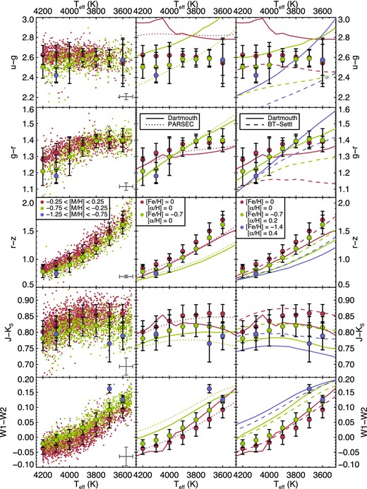
The u − g, g − r, r − z, J − KS, and W1 − W2 colours of APOGEE KM dwarfs as a function of Teff. The left row of panels show data for individual stars, while the middle and right panels show only the mean and standard deviation. The middle panels show APOGEE KM colours compared to Dartmouth and PARSEC models with scaled solar abundances, while the right panels show APOGEE KM colours compared to Dartmouth and BT-Settl colours with α enhanced abundance patterns.
For KM dwarfs with Teff > 3900 K, we find that metal-poor stars have bluer u − g and g − r colours than more metal-rich stars. This is consistent with the pattern for G and K stars, which have blue u − g and g − r colours due to decreased opacity from metal lines in the bluest bands (Roman 1954). For the cooler stars in our sample (3500 < Teff < 3900 K), we find instead that u − g and g − r are constant as a function of both Teff and metallicity. This is not completely consistent with previous results for early-M dwarfs, which indicate that metal-poor M dwarfs have redder g − r colours than their solar metallicity counterparts (West et al. 2004; Lépine & Scholz 2008; Bochanski et al. 2013), tracing a similar effect in to that observed in B − V (Gizis 1997) and B − R (Hartwick 1977). The APOGEE KM sample indicates that the transition from blue metal-poor stars to red metal-poor stars must happen at Teff < 3500 K (∼M2), while each model grid indicates the transition occurs for stars hotter than Teff = 4000 K (the transition between K and M dwarfs). The models are generally a poor match for the data in both u − g and g − r, and applying the 130 K offset derived in Section 2.3 would not improve the agreement.
The r − z colour shows a strong dependence on Teff, as has been demonstrated by previous SDSS work (Bochanski et al. 2010; Dhital et al. 2010). This Teff dependence mimics behaviour previously observed in r − KS and V − K. In addition to the correlation with temperature, r − z shows an offset in metallicity, also recently examined by Bochanski et al. (2013) using the statistical parallax technique. All three model grids reproduce this offset between metal-poor and solar metallicity stars, but there is a shift between the models and data in colour/Teff space. If the 130 K offset derived in Section 2.3 was applied, the overlap between models and data would be significantly better for all isochrones.
For these KM dwarfs, the J − KS (in addition to J − H and H − KS, not shown) colour varies weakly with spectral type/Teff (e.g. Covey et al. 2007; Davenport et al. 2014). The main variable driving variation in these infrared bands is [M/H], a dependence that has been examined for M dwarfs (Leggett 1992; Johnson et al. 2012; Newton et al. 2014). The BT-Settl model grid matches the J − KS colour relatively well, while the Dartmouth and PARSEC grids only reproduce the magnitude of the shift between metallicity bins and not the actual colours. Applying the 130 K offset discussed in Section 2.3 would not result in better agreement between data and models.
The W1 − W2 colour is correlated with both metallicity and temperature, with metal-poor stars having redder colours than their solar metallicity counterparts. While the offset is not large compared to typical WISE photometric uncertainties, because metal-poor stars are red instead of blue, W1 − W2 can be a useful way of disentangling Teff and [M/H] using photometry alone (see Section 5.3). The models generally reproduce the redder colour of metal-poor stars, but do not produce the observed relationship between colour and Teff. In contrast with r − z, the disagreement between the models and the data would become worse if the 130 K offset derived in Section 2.3 was applied.
5.2 Metallicity in colour–colour space
Only two of the photometric metallicity relations derived for KM dwarfs overlap with SDSS-2MASS-WISE photometry used to examine the APOGEE KM sample, a g − r/r − z relation from Bochanski et al. (2013) and a J − KS/H − KS relation from Newton et al. (2014). Fig. 4 shows the KM sample in these two colour–colour spaces compared to both these relations.
![Top row: g − r colour as a function of r − z colour (left and centre panels) and Teff (right panel) for the APOGEE KM sample, with colour indicating metallicity bin. The median and standard deviation g − r colours in each metallicity bin are shown in bins of 0.1 in colour and 100 K Teff. In the centre panel, we also show the Davenport et al. (2014) colour–colour locus and the Bochanski et al. (2013) polynomial fit to g − r as a function of r − z at solar metallicity, in addition to lines for δ(g − r) = 0.04, 0.08, and 0.12. If a linear relationship between δ(g − r) and [M/H] can be assumed, the line colours should match to the metallicity bins; based on the lack of agreement between the δ(g − r) relationship and the APOGEE KM data, a linear relationship is unlikely. Bottom row: J − KS colour as a function of H − KS colour (left and centre panels) and Teff (right panel) for the APOGEE KM sample, with colour indicating metallicity bin. The median and standard deviation g − r colours in each metallicity bin are shown in bins of 0.02 in colour and 100 K Teff. In the centre panel, we also show the Davenport et al. (2014) colour–colour locus and the Newton et al. (2014) metallicity relation are also shown. The reddest and bluest bins for the APOGEE KM sample are likely incomplete.](https://oup.silverchair-cdn.com/oup/backfile/Content_public/Journal/mnras/460/3/10.1093_mnras_stw1139/2/m_stw1139fig4.jpeg?Expires=1750588206&Signature=QM3CjyBlDnwOBLAvQ3IEuWBy74n6tgAhprHCpoASaybCdsxgZP5eNLxWuCZyIwXSDSdfod18kUogZaorf0WKnAlBwEIdzApqTInmRAUvn1y7uYo-HqkZdJ--SsMB-7D5vwKWJq~qtA5TetRphlxZxZsjyVQZk-oa2OgerZni15ZiZr3MA2xj~UDFSSeK0oU2QSXGfz0hNKNgsXk~lTJy01G62tkrTzQq4FGiXNOFGxg1A9~d6OcWfLwSqqiqr52jIjHJGE7mY3DKAd-z4PYqCY9Q~IuLo7VhGJYLPpob5mNca4Tp4cNoqE4WEuDFIh0PPCznm4lFn84B~l82NCSCdA__&Key-Pair-Id=APKAIE5G5CRDK6RD3PGA)
Top row: g − r colour as a function of r − z colour (left and centre panels) and Teff (right panel) for the APOGEE KM sample, with colour indicating metallicity bin. The median and standard deviation g − r colours in each metallicity bin are shown in bins of 0.1 in colour and 100 K Teff. In the centre panel, we also show the Davenport et al. (2014) colour–colour locus and the Bochanski et al. (2013) polynomial fit to g − r as a function of r − z at solar metallicity, in addition to lines for δ(g − r) = 0.04, 0.08, and 0.12. If a linear relationship between δ(g − r) and [M/H] can be assumed, the line colours should match to the metallicity bins; based on the lack of agreement between the δ(g − r) relationship and the APOGEE KM data, a linear relationship is unlikely. Bottom row: J − KS colour as a function of H − KS colour (left and centre panels) and Teff (right panel) for the APOGEE KM sample, with colour indicating metallicity bin. The median and standard deviation g − r colours in each metallicity bin are shown in bins of 0.02 in colour and 100 K Teff. In the centre panel, we also show the Davenport et al. (2014) colour–colour locus and the Newton et al. (2014) metallicity relation are also shown. The reddest and bluest bins for the APOGEE KM sample are likely incomplete.
Bochanski et al. (2013) use δ(g − r) as a proxy for metallicity for M dwarfs, following on previous work (West et al. 2004, 2011) showing that M subdwarfs (classified based on low-resolution optical spectra) have red g − r colours. Bochanski et al. (2013) fit a polynomial to solar metallicity M dwarfs in g − r as a function of r − z, then divide M dwarfs into increasingly metal-poor bins based on δ(g − r), which quantifies how much bluer each M dwarf is than the solar metallicity stars. While the Bochanski et al. (2013) δ(g − r) is correlated to metallicity (as shown through its correlation with ζ, the low-resolution spectroscopic metallicity parameter; Lépine, Rich & Shara 2007; Dhital et al. 2012) it is not explicitly calibrated to metallicity. To compare the APOGEE KM data with the Bochanski et al. (2013) δ(g − r), we used a rough equivalence between δ(g − r) and ζ, then the ζ metallicity relation of Woolf, Lépine & Wallerstein (2009).
The agreement is poor between the Bochanski et al. (2013) relation and the APOGEE KM data. The Bochanski et al. (2013) solar metallicity line does not overlap with the bulk of the APOGEE KM data. The APOGEE KM colours match well with the fiducial colour locus for field stars (Davenport et al. 2014), so the Bochanski et al. (2013) solar metallicity fit was probably based on incomplete data for r − z < 1. The δ(g − r) values also show a strong relationship between colour and metallicity, while the data show g − r is only weakly dependent on metallicity. The δ(g − r) metallicity indicator may not be useful for stars near solar metallicity, and should instead be restricted to the more metal-poor stars ([Fe/H]<−1; subdwarfs and extreme subdwarfs) that were used to derive the indicator.
Newton et al. (2014) use low-resolution infrared lines as metallicity indicators to calibrate a relation based on 2MASS J − KS and H − KS colours, which is compared to the APOGEE KM data in the bottom row of Fig. 4. The Newton et al. (2014) calibration relies on the Bessell & Brett (1988) colour–colour locus (translated to 2MASS bands using Carpenter 2001), then fits an offset in J − KS to metal-poor M dwarfs with blue 2MASS J − KS colours. Again, the agreement between the solar metallicity line and our colours is poor, but the lack of agreement between the APOGEE KM dwarfs and the Davenport et al. (2014) locus indicates that the reddest and bluest bins in H − KS are likely to be biased and/or incomplete for the APOGEE KM sample. This is reasonable, as H − KS is sensitive to both metallicity and Teff and the sample is selected based on Teff. Despite the poor agreement between the solar metallicity locus in colour–colour space, both samples show the same change in J − KS colour due to metallicity (i.e. [M/H] = 0 stars are consistently δ(J − KS) ∼ 0.7 redder than [M/H] = 0.5).
5.3 Empirical Teff and [M/H] relations
While every colour is sensitive to both Teff and [M/H], r − z and W1 − W2 are particularly good tracers of both physical properties. Both r − z and W1 − W2 become redder as a function of Teff and show a strong shift in colour between solar metallicity and metal-poor stars. Classic SDSS [M/H] indicators (u − g and g − r) are degenerate for 3600 < Teff < 3800 K and so are not ideal for these objects, and it is difficult to separate the Teff and [M/H] dependence of 2MASS colours (J − H, J − KS) because their relationship with Teff is weak and non-linear. Because metal-poor stars are blue in r − z and red in W1 − W2, the [M/H]/Teff space is non-degenerate in this colour combination. We provide fits for [M/H] and Teff as a function of both r − z and W1 − W2.
The relationship between [M/H] and these two colours is shown in panel (a) of Fig. 5. The coefficients for the fit to [M/H] as a function of r − z and W1 − W2 are given in Table 6, and the fit is shown with lines of constant [M/H] in panel (a) of Fig. 5. Panel (d) of Fig. 5 shows the fit [M/H] compared to the ASPCAP values. The fit shows a systematic trend with [M/H] but no trend with Teff; the fit is not improved by increasing the polynomial degree. We adopt the scatter in difference between the fit and measured values (0.1 dex) as the uncertainty as it is significantly larger than the formal errors on the fit.
![Relationships between colour, [M/H], and Teff and fit uncertainties for the corresponding fits. Panel (a) (top left) shows W1 − W2 as a function of r − z colour with points coloured according to their [M/H]. Lines of constant [M/H] calculated using the multidimensional fit are shown, and the difference between fit [M/H] and ASPCAP [M/H] as a function of ASPCAP [M/H] is shown in panel (d) (bottom left) with points colour coded according to Teff. Panel (b) (top middle) shows W1 − W2 as a function of r − z colour with points coloured according to their Teff. Lines of constant Teff calculated using the multidimensional fit are shown, and the difference between fit Teff and ASPCAP Teff as a function of ASPCAP Teff is given in panel (e) (bottom middle), colour coded according to [M/H]. Panel (c) (top right) shows Teff as a function of r − z colour with stars colour coded based on their [M/H]. The fit to Teff as a function of r − z and [M/H] is shown for labelled values of [M/H]. Panel (f) (bottom right) shows difference between the Teff calculated from the fit and the ASPCAP Teff value as a function of ASPCAP Teff with points coloured according to [M/H].](https://oup.silverchair-cdn.com/oup/backfile/Content_public/Journal/mnras/460/3/10.1093_mnras_stw1139/2/m_stw1139fig5.jpeg?Expires=1750588206&Signature=z9GlIDjjPIoO3hyIyhegqm9zwyDqXfTaa080PF5bmXIOhrSZ5sxJs7RoRe2AyutDIsJ2qYEg3WeMMr4aypcmrYE6Y05PtYEsUUg7aX5aIUKXz921wLwkByfFBnMkzbgrii-s~IGniY41DZQx5oswDeTI6sgvXqbkNgMbFSubUYc-cY6YC6WGyV1LUHB-X0D4Ef5M6WT0Ru1c4AGSox52NwwFREAU1vzFu8vavlx4o9jgWy0rhXio5TKJziHCnLu6OAHrJ6GBuBAurfdXzmj~MgXxTnZ7zR8KWetG7MHkXHehyVJuCG5L36cEE1KfolN9TKAqRUGh5xAMCvJfZ7Xihw__&Key-Pair-Id=APKAIE5G5CRDK6RD3PGA)
Relationships between colour, [M/H], and Teff and fit uncertainties for the corresponding fits. Panel (a) (top left) shows W1 − W2 as a function of r − z colour with points coloured according to their [M/H]. Lines of constant [M/H] calculated using the multidimensional fit are shown, and the difference between fit [M/H] and ASPCAP [M/H] as a function of ASPCAP [M/H] is shown in panel (d) (bottom left) with points colour coded according to Teff. Panel (b) (top middle) shows W1 − W2 as a function of r − z colour with points coloured according to their Teff. Lines of constant Teff calculated using the multidimensional fit are shown, and the difference between fit Teff and ASPCAP Teff as a function of ASPCAP Teff is given in panel (e) (bottom middle), colour coded according to [M/H]. Panel (c) (top right) shows Teff as a function of r − z colour with stars colour coded based on their [M/H]. The fit to Teff as a function of r − z and [M/H] is shown for labelled values of [M/H]. Panel (f) (bottom right) shows difference between the Teff calculated from the fit and the ASPCAP Teff value as a function of ASPCAP Teff with points coloured according to [M/H].
Coefficients for the relations between colour, Teff, and [M/H].
| Ya | a0 | a1 | a2 | a3 | a4 | σ |
| M/H | −0.822 | 0.634 | – | −4.508 | – | 0.102 |
| |$T_{\rm eff}^b$| | 4707.2 | −958.0 | 226.6 | −1554.2 | 2849.7 | 53.3 |
| Yc | b0 | b1 | b2 | σ | ||
| |$T_{\rm eff}^b$| | 4603.4 | −576.5 | 225.0 | 61.5 |
| Ya | a0 | a1 | a2 | a3 | a4 | σ |
| M/H | −0.822 | 0.634 | – | −4.508 | – | 0.102 |
| |$T_{\rm eff}^b$| | 4707.2 | −958.0 | 226.6 | −1554.2 | 2849.7 | 53.3 |
| Yc | b0 | b1 | b2 | σ | ||
| |$T_{\rm eff}^b$| | 4603.4 | −576.5 | 225.0 | 61.5 |
Note. All relations are only valid 0.8 < r − z < 1.8.
aForm Y = a0 + a1(r − z) + a2(r − z)2 + a3(W1 − W2) + a4(W1 − W2)2;
bASPCAP Teff values were not corrected to match interferometric values;
cform Y = b0 + b1(r − z) + b2[M/H].
The Teff values as a function of r − z and W1 − W2 are shown in panel (b) of Fig. 5. This relationship was best fit by a second degree polynomial in both colours; the coefficients are given in Table 6 and the fit is shown with lines of constant Teff in panel (b) of Fig. 5. The difference between fit Teff and the ASPCAP values is shown in panel (e) of Fig. 5. The scatter in the difference is σ = 53 K, and there are no systematic effects in Teff or [M/H]. While in Section 2.3 we found that ASPCAP Teff is 130 K hotter than the interferometric-based Teff values of Boyajian et al. (2013) and Mann et al. (2015), we did not apply this offset to our Teff values before performing the fit.
We also provide a fit for Teff as a linear function of both r − z and [M/H] for objects with [M/H] measured from other sources.11 The data and associated fit are shown in panel (c) of Fig. 5, and the coefficients are given in Table 6. The difference between ASPCAP Teff and fit Teff is shown in panel (d) of Fig. 5. The linear fit is poor at the high Teff end (Teff > 4100 K), but higher order polynomials did not provide a better fit in that temperature regime. Due to the systematics and the slightly higher scatter (σ = 62 K), this relation should be used only if W1 − W2 photometry is unavailable. Despite the low dispersion on the fits, the precision of these relations is limited uncertainties on the data (σ = 100 K and σ = 0.18 dex).
6 CONCLUSIONS
Precise and accurate determinations of [M/H] and Teff of KM dwarfs based on photometric indicators, especially when combined with upcoming Gaia parallaxes, will revolutionize our understanding of early Galactic evolution. As APOGEE continues to obtain spectra and update the associated model grids, we expect larger numbers of low-mass stars with more accurate parameters. The combination of those values with colours will be very powerful.
We determined that the current ASPCAP catalogue (García Pérez et al. 2015) includes parameters for KM dwarfs with Teff accurate to 100 K (with a 130 K offset) and [M/H] accurate to 0.18 dex. Using those values for the APOGEE KM sample, we examined the relationship between colour, Teff, and [M/H] across SDSS, 2MASS, and WISE bands. We find that nearly every colour shows some sensitivity to Teff and [M/H], though we note that g − r is not very sensitive to metallicity for the cool end of our sample (Teff < 3900 K; corresponding to M0–M2 dwarfs). We confirm strong relationships between [M/H] and colour in r − z, J − KS, and identify W1 − W2 as a metal-sensitive colour over this range.
Comparison to stellar isochrones shows a lack of agreement in most bands, with the poorest agreement in u − g and g − r and better agreement in r − z, J − KS, and W1 − W2. The Bochanski et al. (2013) empirical δ(g − r) [M/H] relation is a poor match with the APOGEE KM data, likely because δ(g − r) was calibrated on subdwarfs, which extend to much lower metallicities than this sample. The Newton et al. (2014) [M/H] relation in J − KS/H − KS space is a better match to APOGEE KM data, but shows an constant shift between lines of the same metallicity. We present the first Teff and [M/H] relationships based on a combination r − z and W1 − W2 colours. These initial relations yield Teff to ∼100 K and [M/H] to ∼0.18 dex precision with colours alone, for Teff in the range of 3550–4200 K and [M/H] in the range of −0.5 to 0.2, and will be substantially improved by refined ASPCAP parameters and an extension to both lower and higher Teff stars.
We thank the anonymous referee whose insightful comments have improved this paper. JAJ also acknowledges support from NSF grant AST-0807997.
This work makes use of data from SDSS-III. Funding for SDSS-III has been provided by the Alfred P. Sloan Foundation, the Participating Institutions, the National Science Foundation, and the US Department of Energy Office of Science. The SDSS-III web site is http://www.sdss3.org/.
SDSS-III is managed by the Astrophysical Research Consortium for the Participating Institutions of the SDSS-III Collaboration including the University of Arizona, the Brazilian Participation Group, Brookhaven National Laboratory, Carnegie Mellon University, University of Florida, the French Participation Group, the German Participation Group, Harvard University, the Instituto de Astrofisica de Canarias, the Michigan State/Notre Dame/JINA Participation Group, Johns Hopkins University, Lawrence Berkeley National Laboratory, Max Planck Institute for Astrophysics, Max Planck Institute for Extraterrestrial Physics, New Mexico State University, New York University, Ohio State University, Pennsylvania State University, University of Portsmouth, Princeton University, the Spanish Participation Group, University of Tokyo, University of Utah, Vanderbilt University, University of Virginia, University of Washington, and Yale University.
This publication also makes use of data products from the Two Micron All Sky Survey, which is a joint project of the University of Massachusetts and the Infrared Processing and Analysis Center/California Institute of Technology, funded by the National Aeronautics and Space Administration and the National Science Foundation.
Additionally, this publication makes use of data products from the Wide-field Infrared Survey Explorer, which is a joint project of the University of California, Los Angeles, and the Jet Propulsion Laboratory/California Institute of Technology, funded by the National Aeronautics and Space Administration.
Table 1 is also available via filtergtaph at https://filtergraph.com/apogee_km_dwarfors.
We note that agreement is similar with the Mann et al. (2015) relation that uses J − H as a metallicity proxy.
We note that while there are stars with data from both surveys, the SEGUE pipeline only produces reliable parameters for warmer stars (Teff > 4500 K; Lee et al. 2008) so SEGUE parameters are not useful calibrators for this APOGEE sample.
Available from the CMD 2.7 input form http://stev.oapd.inaf.it/cmd.
Additional colour/Teff relations can be explored using https://filtergraph.com/apogee_km_dwarfors.
A similar fit for W1 − W2 did not provide accurate Teff values.
REFERENCES
