


Abstract
We examine a model for the variable free–free and neutral hydrogen absorption inferred towards the cores of some compact radio galaxies in which a spatially fluctuating medium drifts in front of the source. We relate the absorption-induced intensity fluctuations to the statistics of the underlying opacity fluctuations. We investigate models in which the absorbing medium consists of either discrete clouds or a power-law spectrum of opacity fluctuations. We examine the variability characteristics of a medium comprised of Gaussian-shaped clouds in which the neutral and ionized matter are co-located, and in which the clouds comprise spherical constant-density neutral cores enveloped by ionized sheaths. The cross-power spectrum indicates the spatial relationship between neutral and ionized matter, and distinguishes the two models, with power in the Gaussian model declining as a featureless power-law, but that in the ionized sheath model oscillating between positive and negative values. We show how comparison of the H i and free–free power spectra reveals information on the ionization and neutral fractions of the medium. The background source acts as a low-pass filter of the underlying opacity power spectrum, which limits temporal fluctuations to frequencies |$\omega \lesssim \dot{\theta }_v/\theta _{\rm src}$|, where |$\dot{\theta }_v$| is the angular drift speed of the matter in front of the source, and it quenches the observability of opacity structures on scales smaller than the source size θsrc. For drift speeds of ∼103 km s−1 and source brightness temperatures ∼1012 K, this limitation confines temporal opacity fluctuations to time-scales of order several months to decades.
1 INTRODUCTION
There is an accumulating body of evidence to suggest that the lines of sight to the compact central regions of some active galaxies exhibit significantly variable absorption due to changes in the column of both neutral and ionized hydrogen. Modelling of the broad-band spectra of PKS 1718-649 over the range 0.15–10 GHz has revealed evidence for changes in its free–free opacity on time-scales of months to years (Tingay & de Kool 2003; Tingay et al. 2015). X-ray observations of the centres of the regions associated with AGN activity exhibit large (>20 per cent) changes in NH on time-scales between days and weeks (Risaliti, Elvis & Nicastro 2002, see also Siemiginowska et al. 2016). There is also some evidence for variations in the H i optical depths of some radio sources (Wolfe, Briggs & Davis 1982; Kanekar & Chengalur 2001).
The interpretation of each of these individual absorption effects has hitherto been treated in isolation. A common theme of existing models involves the passage of clouds across the line of sight to a source which is presumed to be relatively compact in angular extent. Bicknell, Dopita & O'Dea (1997) considered a model for the spectrum of a source obscured by free–free absorption due to a population of clouds whose optical depths follow a power-law distribution, although they did not explicitly compute the statistics of the temporal variations associated with their model. Risaliti et al. (2002) present cloud-based models to account for the variable X-ray photoelectric absorption observed in several sources. As the evidence for H i spectral variability is presently tenuous, there has been little systematic attempt to model it or to deduce its implications for AGN environments, however Briggs (1983) and Macquart (2005) suggest various cloud-based models as explanations.
The purpose of this paper is to present a unified framework for the interpretation of absorption variability towards the cores of radio AGN. The ultimate aim of such an approach is to deduce the composition of the multiphase medium in the vicinity of active nuclei. This presents a means to ascertain what relation exists, if any, between the absorbing structures responsible for the H i, free–free and, ultimately, X-ray absorption. At first glance the basis for the approach may appear unsound because the ionization fraction of the medium might be expected to change rapidly with distance from the nucleus, so that the structures which dominate each type of absorption are physically unconnected. The rapid variability time-scale of X-ray variations suggests that the absorption occurs very close to the central engine, whereas the month- to year-time-scale H i and free–free variations are indicative of larger structures. On the other hand, it is not clear-cut that the medium surrounding the central engine should be cleanly stratified into layers: the turbulent energy that exists in this environment should stir up the medium to prevent a clear delineation of the various phases, so that all phases are spatially co-existent.
A rigorous framework provides the basis on which to interpret the opacity variations to make firm deductions about the veracity of either scenario. In this paper we restrict our analysis to opacity variations at radio wavelengths for two reasons: (i) radio-based diagnostics themselves are sufficient to identify the relation between the distribution of neutral and ionized hydrogen, and (ii) there are likely to be strong differences in the structure and location of the X-ray and radio-emitting background sources which would hinder quantitative comparison of the absorption diagnostics. Nevertheless, we remark that, although X-ray observations of AGN have been undertaken with day to week cadences, radio observations of spectral variability due to free–free and H i absorption processes have not been made with such high cadences. This paper explores the motivation to investigate this observational regime.
The paper is organized as follows. In Section 2 we present a general model for absorption by an ensemble of clouds. In Section 3 we link the characteristics of the clouds with their ensemble-average variability properties. We use this model to explore the significance of temporal variability between the various absorption-based radio-wavelength diagnostics. In Section 4 we demonstrate how the model may be used to glean information from existing variability data. Our conclusions are presented in Section 5.
2 TEMPORAL SPECTRA OF ABSORPTION FLUCTUATIONS
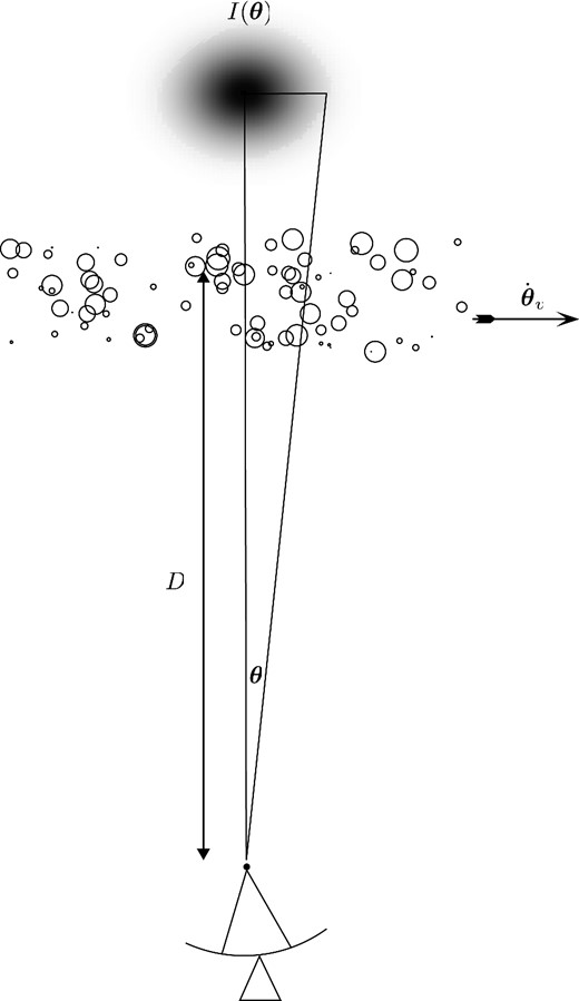
A depiction of the geometry of the absorption model. The absorbing material is located on a thin plane at an angular diameter distance D from the observer, and drifts across the line of sight at an angular velocity |$\dot{\boldsymbol {\theta }}_v$|. The absorbing structure is view against a bright compact source with brightness distribution |$I(\boldsymbol {\theta })$|.
The foregoing formalism also admits in a restricted sense the treatment of opacity fluctuations associated with any relativistic synchrotron-emitting gas that may be present in the foreground of the radio source. Specifically, we may examine the distribution of relativistic gas in the vicinity of the H i and free–free absorbing media using this formalism if the brightness temperature of the synchrotron-emitting gas is substantially less than that of the background source. In this instance we may treat the fluctuations in the synchrotron optical depth in a similar manner to the free–free opacity variations in our formalism below.
In general the exact angular distribution of τ is unknown a priori, but it is possible to describe the temporal flux density variations in terms of the corresponding power spectrum, or cross-power spectrum when comparing absorption at two different frequencies, ν and ν′. The power spectrum characterises the temporal variations associated with H i or free–free absorption alone. The cross-power spectrum compares H i absorption intensity changes with intensity changes due to the free–free opacity. The objective is to relate the temporal spectrum to the underlying statistical properties of the opacity distributions.
The effect of the integral over |$I(\boldsymbol {\theta })$| in equation (8) is to act as a low-pass spectral filter. This has two effects on the spectrum: it removes high frequency temporal fluctuations and it suppresses the overall amplitude of the variability. A source of finite characteristic size θsrc strongly attenuates frequencies |$\omega \gtrsim \dot{\theta }_v / \theta _{\rm src}$| in the temporal power spectrum. One does not therefore expect opacity-induced intensity variations on time-scales considerably less than the source crossing time |$t_{\rm char} \sim \theta _{\rm src}/\dot{\theta }_v$|. Source size further attenuates the overall amplitude of the variability: a finite source only admits spatial frequencies |$q_\perp \lesssim \theta _{\rm src}^{-1}$|, so that the integral over q⊥ only samples the power contained in opacity fluctuations on angular scales larger than ∼θsrc.
To the extent there is no cross-correlation in the underlying opacity fluctuations, no correlated variability will be observed. We remark that one may equally investigate the foreground of synchrotron-absorbing relativistic gas as free–free absorption by substituting νff for νsynch, subject to the caveats discussed below equation (1).
The underlying spectra of H i and free–free opacity fluctuations are unknown in general. To gain further insight into the physics we introduce specific models for the structure of the medium in the following section.
3 ABSORPTION BY AN ENSEMBLE OF CLOUDS
The particular choice of a specific model, involving an ensemble of discrete clouds for the structure of the absorbing region, is adopted here because it connects in a theoretical sense to the work of Bicknell et al. (1997) in terms of the modelling of GPS/CSS radio spectra. Some numerical simulations of such a scenario have also been explored, by Saxton et al. (2005). The success of the theoretical and simulation approaches, against observational data, indicate that this choice has significant future promise that may be relevant for free–free, H i, and X-ray absorption, as similar suggestions have been made for X-ray absorption by Risaliti et al. (2002) and for H i absorption by Briggs (1983).
Let us apply the foregoing results to the specific case of absorption by an ensemble of clouds. We determine the power spectra |$\Phi _\tau ({\boldsymbol {q}},\nu ,\nu ^{\prime })$| for clouds comprised of an admixture of neutral and ionized material. We parametrize the density associated with each cloud, given by a function |$T({\boldsymbol {\theta }}-\Delta \boldsymbol {\theta },z;\theta _{\rm c})$|, in terms of its size θc and its angular offset, |$\Delta \boldsymbol {\theta }$|, from the line of sight at time t = 0, where z is the coordinate parallel to the line of sight.
The positions and sizes of the clouds are unknown, but we can compute an average over these quantities to determine the average power and cross-power spectrum of the optical depth. In the following subsections we explore various averages over these quantities.
3.1 Average over cloud positions
The important result of this section is that, if clustering is unimportant, only the self-terms of each cloud contribute on average to the power spectrum of intensity variations.
3.2 Specific cloud models
3.2.1 Gaussian profile
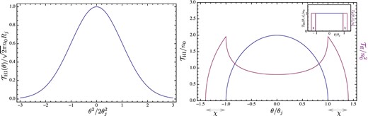
The column profiles of the two models investigated here. Left: the H i column density for the Gaussian cloud model (with the ionized component following the same functional form). Right: the column densities of the neutral and ionized components of the shell model, with (inset, top right) a plot of the corresponding angular dependence of |$T_{\rm H\,\small {I}}(\theta ,z)$| and Tff(θ, z) from which the column profiles are derived.
The generic nature of each spectrum, as illustrated in Fig. 3 is as follows: the spectrum is flat for |$0<q<\theta _{\rm max}^{-1}$|, follows a power-law decline with index γ − 7, and then the spectrum declines sharply for |$q>\theta _{\rm min}^{-1}$|. The simplification enabled by neglect of clustering thus offers a straightforward means of extracting the parameters A and B which encapsulate the physics of the neutral and ionized medium fractions within each cloud, as we discuss further in Section 4.
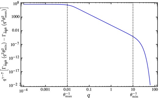
The generic behaviour of the spectra in equations (21), here plotted with γ = 3, θmax = 100 and θmin = 0.1.
3.2.2 Neutral clouds with ionized shells
Simulations of jet environments, e.g. Saxton et al. (2005), can model the medium in the vicinity of an AGN as composed of clouds which are abraded by the AGN jet. We are thus motivated to consider the opacity fluctuations associated by an ensemble of clouds whose neutral hydrogen cores extend to some radius R and whose ionized outer layer extends in a thin shell from a radius R to a radius R(1 + χ).
These expressions may be integrated over a power law distribution of cloud radii to obtain the ensemble-average power- and cross-spectra of the opacity. Although the model is simple, the analytic forms of the resulting power spectra are algebraically cumbersome, so we present them in Appendix A and describe the results in general terms here. The general behaviour of the spectra is shown in Fig. 4, and is described as follows.
The H i and free–free power spectra are flat over the range |$0<q \lesssim 0.5 \, \theta _{\rm max}^{-1}$|, where we recall that θmax is the maximum cloud size.
For γ < 3 the power spectrum declines as q−4 for |$q> \theta _{\rm max}^{-1}$|. For size distributions with γ > 3, the spectrum is dominated by θmin, and it declines as q−4 once |$q > \theta _{\rm min}^{-1}$|.
The presence of the thin-shelled structure in the free–free angular distribution introduces ringing in the power spectrum with a characteristic ripple length q ∼ [θmax(1 + χ)]−1.
The cross-power spectrum is approximately flat for |$q \lesssim 0.5 \,\theta _{\rm max}^{-1}$|, but for γ < 3 and |$q \gtrsim 0.5\, \theta _{\rm max}^{-1}$| the cross power oscillates between positive and negative values, and is bounded by an envelope whose amplitude scales as q−4.
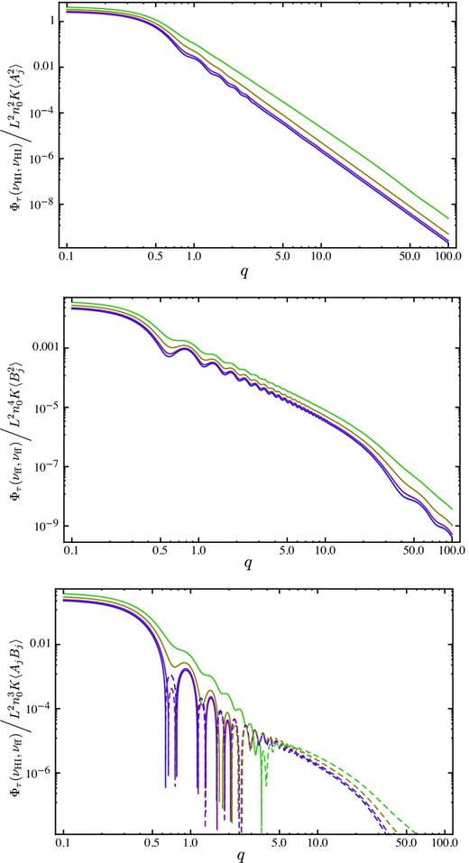
The H i power spectrum, free–free power spectrum, and HI-free–free cross-power spectrum for the ionized sheath model. The spectra are plotted here with parameters θmin = 0.01, θmax = 1.0 and χ = 0.03. In the cross-power spectrum negative values are denoted by dotted lines. The different curves denote the spectra for γ = 0.5, 1.01, 2 and 3.01 (in order of increasing amplitude).
3.3 Temporal behaviour for power-law opacity spectra
Having derived the two-dimensional power and cross-power spectra of the opacity-induced intensity fluctuations, we would like to relate these back to the observables, namely the spectra of temporal intensity fluctuations.
As discussed in Section 2, the derivation of the spectrum of temporal intensity fluctuations involves integration of the product of the power (or cross-) spectrum with the source brightness power (cross-) spectrum over the coordinate orthogonal to the drift velocity, q⊥ (see equations 8 and 9). Although derivation of the temporal power spectrum is complicated by its dependence on source size, which is in principle not known in detail, it is a possible to incorporate the effect of source size by approximating the brightness profile with a Gaussian form with characteristic size θsrc(ν), which we write explicitly as a function of observing frequency ν.
For a source with a brightness profile |$I(\boldsymbol {\theta };\nu ) = I_0(\nu ) \exp [ -\theta^2\!/\theta _{\rm src}^2(\nu ) ]$|, the Fourier-transformed brightness is of the form |$\tilde{I}({\boldsymbol {q}};\nu ) = {\cal I}(\nu ) \exp [-q^2 \theta _{\rm src}^2(\nu )/4]$|, with |${\cal I}(\nu ) = I_0(\nu ) \, \pi \theta _{\rm src}^2(\nu )$|. Thus the spatial power spectrum cuts off at |$q_{\rm src}^2 =2/\theta _{\rm src}(\nu )^2$|, and the cross-spectrum measured between frequencies ν and ν′ cuts off at |$q_{\rm src}^2 = 4/[\theta _{\rm src}^2(\nu ) + \theta _{\rm src}^2(\nu ^{\prime })]$|.
The detailed calculation of the temporal power spectrum is presented in Appendix B, and we summarize the results here. The generic shape of the spectrum is shown in Fig. 5. The temporal power spectrum is approximately flat for angular frequencies |$0 < \omega /\dot{\theta }_v < q_{\rm min}$| and then declines as ω1−β until the source size cuts the spectrum off near |$\omega /\dot{\theta }_v \approx q_{\rm src}$|. The power-law portion of the spectrum is not evident if the source is sufficiently large, qsrc < qmin (i.e. if the angular size of the source exceeds the outer scale of the fluctuations in optical depth).
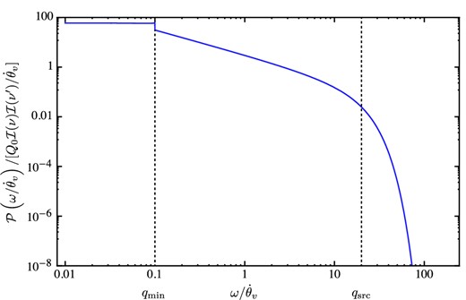
An illustration of the temporal power spectrum associated with an opacity spatial power spectrum whose index is β = 2, plotted here for an opacity power spectrum whose low-spatial frequency cutoff is qmin = 0.1 and for a source size which cuts the spatial power spectrum off at qsrc = 20.
3.3.1 Temporal cross-spectrum for clouds with ionized sheaths
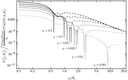
The temporal cross-power spectrum of variations between H i and free–free absorption in the ionized sheath model for a distribution of cloud sizes proportional to θ−2, with a maximum cloud size of θmax = 1.0 and a minimum size of θmin = 0.01, for various fractional sheath thicknesses χ.
4 DISCUSSION
In principle measurements of the temporal spectra of opacity variations due to H i and free–free absorption in front of compact radio sources offer a means of discerning the fine-scale spatial structure of the media in external galaxies, and the cross-power spectrum offers a means of discerning the relationship between the spatial distribution of their neutral and ionized phases.
However, two factors hamper our ability to determine the details of the spatial distribution from temporal opacity variations: the first is that the temporal variations integrate over the spectrum of spatial fluctuations in the direction orthogonal to the drift velocity. This partially smooths over any features in the spectrum that are indicative of the detailed distribution of absorbing structure: the amplitude of features in the temporal spectrum is reduced relative to that in the spatial spectrum.
The second effect is that of the finite size of the background source, which cuts off the temporal power spectrum at an angular frequency |$\omega = \dot{\theta }_v /\theta _{\rm src}$|. The background source effectively acts as a low-pass filter of spatial information. This latter effect poses a serious limitation to measurements of the interrelation between neutral and ionized matter if the differences in their distribution occur only on angular scales finer than θsrc. Our examination of the results of two contrasting cloud models introduced above illustrates this point.
We have considered several models in which absorbing clouds are distributed randomly without clustering and whose sizes follow a power law distribution with index −γ. In the Gaussian cloud model the density of ionized and neutral matter both decline as a Gaussian from the cloud centre (i.e. the two phases are inter-mixed on tiny scales), and the spectra of temporal flux density variations associated with both H i and free–free absorption are essentially featureless: they are both flat in the range |$0 < \omega < \dot{\theta }_v/\theta _{\rm max}$|, and then either decline as ωγ−6 until |$\omega > \dot{\theta }_v/\theta _{\rm min}$| or they decline at |$\omega > q_{\rm src} \dot{\theta }_v \approx \theta _{\rm src}^{-1} \dot{\theta }_v$|, the point at which the finite source size hampers our ability to discern finer detail in the absorbing medium. In practice, we certainly expect the background source to possess a greater angular size than θmin, and possibly also θmax: the ωγ−6 portion of the spectrum may not be discernible for all sources.
The ionized sheath model is distinguishable from the Gaussian model on temporal frequencies |$\omega \gtrsim \dot{\theta }_v/\theta _{\rm max}$|, whereupon the power- and cross-spectra begin to oscillate on scales |$\omega \sim \dot{\theta }_v / \theta _{\rm max} (1+\chi )$|. For γ < 3 the amplitude of the envelope of oscillations in the power spectrum declines as ω−3 for |$\omega > \theta _{\rm max}^{-1} \dot{\theta }_v$|.
If the linear extent of the background source is large compared to the outer scale of the power spectrum, equivalent to the largest cloud size in the discrete cloud models, the temporal spectrum of opacity-induced intensity fluctuations will be flat for all temporal frequencies up to a value |$\omega \sim \dot{\theta }_v/\theta _{\rm src}$|, and will cut-off sharply at higher frequencies. This case applies to absorption against bright (Sν > 1 Jy) distant (D > 100 Mpc) radio sources with vapp ≪ c.
where 〈Xj〉 is the neutral fraction averaged all the clouds (subscripted by the index j) and 〈Yj〉 is related to the ionization fraction of the clouds, as described in equations (13) and (15). Thus we see that the relative amplitudes of the temporal power- and cross-spectra yield information on the ensemble-average neutral and ionized fractional content of the medium.
We stress that the underlying spatial power- and cross-spectra of H i and free–free opacity variations should be regarded as the fundamental quantities of interest. In this sense the two cloud models considered in this paper represent extremes of a range of possible models for the spatial distribution of ionized and neutral material in the circumnuclear regions of external galaxies. These models for the spatial distribution of matter provide a means of forward-modelling the temporal spectra, and their purpose is to provide a physical context in which to interpret the results of the temporal variations.
4.1 Application to PKS 1718–649
As an illustration of the foregoing results, we consider the nearby (z = 0.0144, D = 57.7 Mpc) GPS source PKS 1718−649, whose changes in flux density and spectral shape in the range 1–3 GHz were interpreted as evidence of variations in the free–free opacity by Tingay et al. (2015). The source was observed at three epochs over a 21 month period, and the 0.5 Jy flux density change observed at 1 GHz over this period implies an opacity change of Δτ ≳ 0.13. Parkes observations at 725 MHz and MWA observations at 199 MHz further constrain the spectral shape and appear to exclude simple models that involve homogeneous absorbing material. This provides strong motivation to consider whether spatial inhomogeneity in the free–free opacity in the foreground of the source is consistent with the temporal variations observed.
5 CONCLUSION
We have presented a formalism for interpreting the temporal variations in H i and free–free opacity observed in some young, compact radio sources and for connecting these with the underlying properties of the circumnuclear media of their host galaxies. The theory is, however, more widely applicable to any medium comprised of ionized and neutral material drifting in front of a radio source at a fixed velocity.
The background source structure acts as a low pass filter on the opacity variations observable against these sources and limits the time-scales of variations and minimum size of the structures probed within the medium. For drift rates of ∼103 km s−1 against sources of brightness temperatures ∼1012 K the expected time-scale of variability is of order years to decades. Much faster variations are possible against radio-emitting outbursts with apparently superluminal speeds, giving rise to variations on time-scales ≳ 300 times smaller (i.e. of order days to weeks). However, such motions are not thought to be relevant to some young radio sources in which free–free opacity variations are believed to occur (e.g. Tingay et al. 2015). The expected time-scale is potentially an important distinguishing feature of this model relative to other proposed variability mechanisms, particularly those related to interstellar scintillation, which typically gives rise to variations on day to several-week time-scales; apparent absorption variations can result from the scintillation of the flux density associated with any fine-scale angular structure imprinted in the image of a source by structure in the foreground absorbing medium. We refer the reader to Macquart (2005) for a more detailed discussion as it applies to several-week time-scale variations in H i.
Measurements of the power- and cross-power spectrum of intensity fluctuations associated with the H i and free–free opacity variations can resolve the nature of the spatial relationship between the two phases. We have investigated two contrasting models for their distribution – one based on clouds with Gaussian density profiles, and another based on clouds comprised of neutral cores with ionized sheaths – and shown how the power spectra of temporal intensity fluctuations differs between the two cases. However, source structure limits the angular scales accessible to ≳ θsrc so that, if the ionized and neutral medium is predominately distinguishable only on scales smaller than this, then these scales will not be accessible through measurements of temporal opacity fluctuations. However, even in this case it is still possible to discern details about the average ionization and neutral fraction of the medium through comparison of the H i and free–free opacity temporal variations. Specifically, comparison of the amplitudes of the power spectra of intensity fluctuations caused by these two absorption mechanisms reveals the ratio |$n_0^{-2} \langle X^2 \rangle /\langle Y^2 \rangle$|, where X is the neutral fraction and Y is the ionization fraction relative to the overall density, n0. The amplitude of the cross-power spectrum between H i and free–free intensity variations relative to the free–free power spectrum further reveals the quantity |$n_0^{-1} \langle Y \rangle /\langle X \rangle$|.
Finally, we note that there are exciting prospects for undertaking future investigations of the interstellar media of young compact extragalactic radio sources. Facilities such as the MWA (Lonsdale et al. 2009; Tingay et al. 2013) are capable of making extremely sensitive measurements of variations in free–free opacity at the low frequencies, ∼80–250 MHz, at which the effects of free–free absorption are easily measurable. Meanwhile, cm-wavelength facilities such as ASKAP (Johnston et al. 2007, 2008) are capable of undertaking large surveys for radio galaxies with variable H i absorption (Allison et al. 2015) and, with its high spectral stability and dynamic range, in measuring extremely small opacity variations.
Parts of this research were conducted by the Australian Research Council Centre of Excellence for All-sky Astrophysics (CAASTRO), through project number CE110001020.
The assumption of normality has a proven pedigree in a number of closely-related fields [e.g. for the statistics of the column density of ionized plasma in our Galaxy's interstellar medium (ISM)] in successfully predicting various observables (e.g. the scatter-broadening of compact radio sources). As the H i optical depth is also linear in the matter density, it seems reasonable to adopt this approximation here. To the extent that fluctuations in the ionized density of our own ISM follow a normal distribution, variations in τff, though quadratic in the local density, might similarly be expected to exhibit statistics closely approximating that of a normal distribution, even if only by virtue of the central limit theorem. Moreover, even when the opacity is not normally distributed, the result for 〈exp (−τ)〉 used here is still correct to second order in τ. Significant differences are only evident for τ ≫ 1, a condition unlikely to be relevant here (see text below).
Of course, it is possible for H i and free–free absorption to occur at the same frequency, even though the foregoing theory treats their effects separately. This approach is justified because the effect of the two is observationally separable: an observational analysis would separate H i absorption variations from free–free absorption absorption because the H i flux density variations are measured with respect to the nearby continuum spectrum (which may be subject to free–free absorption).
This treatment follows the formalism introduced in Macquart (2005) in another context, which we recap here for completeness, but to which we refer the reader for additional details.
REFERENCES
APPENDIX A: THE POWER AND CROSS-POWER SPECTRA OF CLOUDS WITH A NEUTRAL CORE AND IONIZED SHEATH
APPENDIX B: THE TEMPORAL POWER SPECTRUM
In this Appendix we compute the temporal power spectrum associated with a medium whose spatial opacity power spectrum follows a power law, of the form given in equation (24). In this treatment we consider the effect of finite source size by modelling the source as a Gaussian which cuts the spatial power spectrum off at a scale qmax, as discussed in Section 3.3 above.
