


Abstract
We report on 22 yr of radio timing observations of the millisecond pulsar J1024−0719 by the telescopes participating in the European Pulsar Timing Array (EPTA). These observations reveal a significant second derivative of the pulsar spin frequency and confirm the discrepancy between the parallax and Shklovskii distances that has been reported earlier. We also present optical astrometry, photometry and spectroscopy of 2MASS J10243869−0719190. We find that it is a low-metallicity main-sequence star (K7V spectral type, [M/H] = −1.0, Teff = 4050 ± 50 K) and that its position, proper motion and distance are consistent with those of PSR J1024−0719. We conclude that PSR J1024−0719 and 2MASS J10243869−0719190 form a common proper motion pair and are gravitationally bound. The gravitational interaction between the main-sequence star and the pulsar accounts for the spin frequency derivatives, which in turn resolves the distance discrepancy. Our observations suggest that the pulsar and main-sequence star are in an extremely wide (Pb > 200 yr) orbit. Combining the radial velocity of the companion and proper motion of the pulsar, we find that the binary system has a high spatial velocity of 384 ± 45 km s−1 with respect to the local standard of rest and has a Galactic orbit consistent with halo objects. Since the observed main-sequence companion star cannot have recycled the pulsar to millisecond spin periods, an exotic formation scenario is required. We demonstrate that this extremely wide-orbit binary could have evolved from a triple system that underwent an asymmetric supernova explosion, though find that significant fine-tuning during the explosion is required. Finally, we discuss the implications of the long period orbit on the timing stability of PSR J1024−0719 in light of its inclusion in pulsar timing arrays.
1 INTRODUCTION
The recent direct detection of gravitational waves by ground-based interferometers has opened a new window on the Universe (Abbott et al. 2016). Besides ground-based interferometers, gravitational waves are also predicted to be measurable using a pulsar timing array (PTA), in which an ensemble of radio millisecond pulsars are used as extremely stable, celestial clocks representing the arms of a Galactic gravitational wave detector (Detweiler 1979; Hellings & Downs 1983).
At present, three PTAs are in operation; the European Pulsar Timing Array in Europe (EPTA; Desvignes et al. 2016), the Parkes Pulsar Timing Array (PPTA) in Australia (Manchester et al. 2013) and NANOGrav in North-America (Demorest et al. 2013). The three PTAs have been in operation for about a decade, and have so far provided limits on the stochastic gravitational wave background at nano-hertz frequencies (e.g. Shannon et al. 2013; Arzoumanian et al. 2015; Lentati et al. 2015). The three PTAs collaborate together as the International Pulsar Timing Array (IPTA; Verbiest et al. 2016). As a result of improvements in instrumentation, analysis software, and higher observing cadence, the timing precision has increased with time, which leads previously unmodelled effects to become important.
The first data release by the EPTA (EPTA DR1.0) has recently been published by Desvignes et al. (2016) and provides high-precision pulse times-of-arrival (TOAs) and timing ephemerides for an ensemble of 42 radio millisecond pulsars spanning baselines of 7–18 yr in time. While preparing this data release, we rediscovered the apparent discrepancy in the distance of the isolated millisecond pulsar J1024−0719 which was reported by Espinoza et al. (2013) and also noticed by Matthews et al. (2016). This discrepancy arises due to the high proper motion of the pulsar, which gives rise to an apparent positive radial acceleration and hence a change in the spin period known as the Shklovskii effect (Shklovskii 1970). In the case of PSR J1024−0719, the Shklovskii effect exceeds the observed spin period derivative for distances larger than 0.43 kpc. Pulsar timing yields parallax distances beyond that limit, which would require an unphysical negative intrinsic spin period derivative for PSR J1024−0719.
This discrepancy could be resolved through a negative radial acceleration due to a previously unknown binary companion in a very wide orbit. In a search for non-thermal emission from isolated millisecond pulsars, Sutaria et al. (2003) studied the field of PSR J1024−0719 in optical bands. Their observations revealed the presence of two stars near the position of the pulsar. The broad-band colours and spectrum of the bright star, 2MASS J10243869−0719190 (R ∼ 19, hereafter star B) were consistent with those of a main-sequence star of spectral type K5, while the other, fainter star (R ∼ 24, hereafter star F) had broad-band colours which Sutaria et al. (2003) suggested could be consistent with non-thermal emission of the neutron star (NS) in PSR J1024−0719. However, the astrometric uncertainties in both the optical and radio did not allow Sutaria et al. (2003) to make a firm conclusion on the association of either stars B or F and PSR J1024−0719.
Here, we present radio observations of PSR J1024−0719 and optical observations of stars B and F (Section 2) that allow us to improve the timing ephemeris of PSR J1024−0719 and the astrometry, photometry and spectroscopy of stars B and/or F (Section 3). In Section 4, we present our results which show that star B is in an extremely wide orbit around PSR J1024−0719. An evolutionary formation scenario for this wide orbit is presented in Section 5. We discuss our findings and conclude in Section 6. This research is the result of the common effort to directly detect gravitational waves using pulsar timing, known as the EPTA (Desvignes et al. 2016).1
While preparing this paper, we became aware that a different group had used independent radio timing observations and largely independent optical observations to reach the same conclusion about the binarity of PSR J1024−0719 (Kaplan et al. 2016). The analysis and results presented in this paper agree very well with those of Kaplan et al. (2016), though these authors suggest an alternate formation scenario for PSR J1024−0719 (see Section 5.4).
2 OBSERVATIONS
2.1 Radio
We present radio timing observations of PSR J1024−0719 that were obtained with telescopes participating in the EPTA over the past 22 yr. The EPTA DR1.0 data presented by Desvignes et al. (2016) contains timing observations of PSR J1024−0719 from the ‘historical’ pulsar instrumentation at Effelsberg, Jodrell Bank, Nançay and Westerbork and contains 561 TOAs over a 17.3 yr time span from 1997 January to 2014 April.
The DR1.0 data set was extended back to 1994 March with observations obtained at 410, 610 and 1400 MHz with the Jodrell Bank analog filterbank (AFB; Shemar & Lyne 1996). The first year of this data set has been published in the PSR J1024−0719 discovery paper by Bailes et al. (1997). We also included observations obtained with the new generation of baseband recording/coherent dedispersing pulsar-timing instruments presently in operation within the EPTA. These instruments are PuMa II at Westerbork (Karuppusamy, Stappers & van Straten 2008), PSRIX at Effelsberg (Lazarus et al. 2016), the ROACH at Jodrell Bank (Bassa et al. 2016) and BON and NUPPI at Nançay (Cognard & Theureau 2006; Cognard et al. 2013). A subset of the Nançay TOAs on PSR J1024−0719 were presented in Guillemot et al. (2016). Combining these data sets yields 2249 TOAs spanning 22 yr since the discovery of PSR J1024−0719 (Table 1 and Fig. 1).
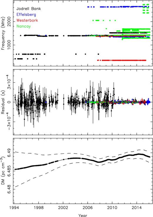
Radio timing observations at different observing frequencies are shown in the top panel as a function of time. Observations from different observatories are shown in different colours. The middle panel shows timing residuals of PSR J1024−0719 based on our timing ephemeris (Table 1). The bottom panel shows the DM values as modelled by the power-law model. The dashed lines indicate the uncertainty in the DM.
Parameters for PSR J1024−0719. All reported uncertainties have been multiplied by the square root of the reduced χ2.
| Fit and data set | |
|---|---|
| MJD range | 49416.8–57437.0 |
| Data span (yr) | 21.96 |
| Number of TOAs | 2249 |
| Rms timing residual (μs) | 2.81 |
| Weighted fit | Y |
| Reduced χ2 value | 0.98 |
| Reference epoch (MJD) | 55000 |
| Measured quantities | |
| Right ascension, αJ2000 | |$10^\mathrm{h}24^\mathrm{m}38{^{\rm s}_{.}}675\,380(5)$| |
| Declination, δJ2000 | |$-07^\circ 19^\prime 19{^{\prime\prime}_{.}} 433\,96(14)$| |
| Proper motion in RA, μαcos δ (mas yr−1) | −35.255(19) |
| Proper motion in Dec., μδ (mas yr−1) | −48.19(4) |
| Parallax, π (mas) | 0.77(11) |
| Pulse frequency, f (s−1) | 193.715 683 448 5468(7) |
| First derivative of f, |$\dot{f}$| (s−2) | −6.958 93(15) × 10−16 |
| Second derivative of f, |$\skew4\ddot{f}$| (s−3) | −3.92(2) × 10−27 |
| Third derivative of f, f(3) (s−4) | <2.7 × 10−36 |
| Fourth derivative of f, f(4) (s−4) | <4.5 × 10−44 |
| Dispersion measure, DM (pc cm−3) | 6.4888(8) |
| First derivative of DM (pc cm−3 yr−1) | 3(15) × 10−5 |
| Second derivative of DM (pc cm−3 yr−2) | −1.4(1.8) × 10−5 |
| Assumptions | |
| Clock correction procedure | TT(BIPM2011) |
| Solar system ephemeris model | DE421 |
| Units | TCB |
2.2 Optical
We retrieved imaging observations of the field of PSR J1024−0719 from the ESO archive. These observations consist of 3 × 2 min V-band, 3 × 3 min R-band, and 3 × 2 min I-band exposures, which were obtained with the FORS1 instrument (Appenzeller et al. 1998) at the ESO VLT at Cerro Paranal on 2001 March 28 under clear conditions with 0.6 arcsec seeing. The high-resolution collimator was used, providing a 0.1 arcsec pix−1 pixel scale and a 3.4 arcsec × 3.4 arcsec field of view. Photometric standards from the Landolt (1992) SA109 field were observed with the same filters and instrument setup. Analysis of this data has been presented by Sutaria et al. (2003).
The field of PSR J1024−0719 was also observed with OmegaCAM (Kuijken 2011) at the VLT Survey Telescope. OmegaCAM consists of 32 4 k × 2 k CCDs with a 0.21 arcsec pix−1 pixel scale. SDSS ugriz observations were obtained between 2012 February 24 and March 2 as part of the ATLAS survey (Shanks et al. 2015). Here, we specifically use the 45 s SDSS r-band exposure obtained on 2012 February 27. The seeing of that exposure was 0.75 arcsec.
Follow-up observations of the field of PSR J1024−0719 were taken on 2015 June 10 and 11 with FORS2 at the ESO VLT at Cerro Paranal in Chile. A series of eight dithered 5 s exposures in the R-band filtered were obtained on June 10, under clear conditions with mediocre seeing of 1.1 arcsec. The standard resolution collimator was used with 2 × 2 binning, providing a pixel scale of 0.25 arcsec pix−1 with a 6.8 arcmin × 6.8 arcmin field of view.
Two long-slit spectra were also obtained with FORS2, one with the 600RI grism on June 10 and one with the 600z grism on June 11. These grisms cover wavelength ranges of 5580–8310 Å and 7750–10 430 Å, respectively. Both exposures were 1800 s in length and used the 1.0 arcsec slit. The CCDs were read out using 2 × 2 binning, providing a resolution of 6.3 Å, sampled at 1.60 Å pix−1 for both the 600RI and 600z grism. The seeing during these exposures was 0.77 and 0.80 arcsec, respectively. The spectrophotometric standard LTT 3864 was observed with the same grisms and a 5 arcsec slit. Arc-lamp exposures for all grism and slit combinations were obtained as part of the normal VLT calibration programme.
3 ANALYSIS
3.1 Pulsar timing
We use the standard approach, as detailed in Edwards, Hobbs & Manchester (2006), for converting the topocentric TOAs to the Solar-system barycenter through the DE421 ephemeris (Folkner, Williams & Boggs 2009) and placing them on the Terrestrial Time standard (BIPM2011; Petit 2010). The TOAs from the different combinations of telescope and instrument were combined in the tempo2 pulsar timing software package (Hobbs, Edwards & Manchester 2006).
The best-fitting timing solution to the TOAs was found through the standard tempo2 iterative least-squares minimization. The free parameters in the fit consist of the astrometric parameters (celestial position, proper motion and parallax), a polynomial describing the spin frequency f as a function of time, and a polynomial to describe variations in the pulsar dispersion measure (DM) as a function of time. We also fitted for offsets between the telescope and instrument combinations to take into account difference in pulse templates and instrument delays.
To perform model selection between models that include increasing numbers of spin frequency derivatives when incorporating increasingly complex noise models, we use the Bayesian pulsar timing package temponest (Lentati et al. 2014), which operates as a plugin to tempo2. In all cases, we include parameters to model the white noise that scale, or add in quadrature with, the formal TOA uncertainties, and define these parameters for each of the 20 observing systems included in the data set. We also include combinations of additional time correlated processes, including DM variations and system-dependent noise. For this final term, we use the approach described in Lentati et al. (2016). Apart from the spin frequency, derivatives we marginalize over the timing model analytically. The spin frequency derivatives are included in the analysis numerically with priors that are uniform in the amplitude of the parameter in all cases.
When including only white noise parameters, and limiting our model for DM variations to a quadratic in time, we find the evidence supports a total of four frequency derivatives. However, we find there is significant support from the data for higher order DM variations. In particular, the difference in the log evidence for models with and without an additional power-law DM model besides the quadratic model is 36 in favour of including the additional stochastic term. We find the spectral index of the DM variations (3.2 ± 0.6) to be consistent with that expected for a Kolmogorov turbulent medium. When including these additional parameters to describe higher order DM variations, we find that the data only support the first and second frequency derivatives. The significant detections of the third and fourth frequency derivatives observed in the simpler model can therefore not be confidently interpreted as arising from a binary orbit, as they are highly covariant with the power-law variations in DM, thereby reducing their significance. Finally, we find no support for any system-dependent time-correlated noise in this data set. The timing ephemeris using a DM power-law model is tabulated in Table 1 and timing residuals and DM values as a function of time are plotted in Fig. 1.
3.2 Photometry
The FORS1 and FORS2 images were bias-corrected and flat-fielded using sky flats. Instrumental magnitudes were determined through point spread function (PSF) fitting with the daophot II package (Stetson 1987). The instrumental PSF magnitudes of the 2001 VRI observations were calibrated against 17 photometric standards from the SA109 field, using calibrated values from Stetson (2000) and fitting for zero-point offsets and colour terms, but using the tabulated ESO extinction coefficients of 0.113, 0.109 and 0.087 mag airmass−1 for VRI, respectively. The residuals of the fit were 0.03 mag in V, 0.06 mag in R and 0.07 mag in I. We find that star B has V = 19.81 ± 0.04, R = 18.78 ± 0.06 and I = 18.00 ± 0.07, while star F has V = 24.71 ± 0.13, R = 24.64 ± 0.14 and I = 24.57 ± 0.34.
The instrumental magnitudes of the eight FORS2 R-band images from 2015 were calibrated against the 2001 FORS1 observations. As the FORS2 R-band (R_SPECIAL) filter has a different transmission curve compared to the FORS1 Bessell R-band (R_BESS) filter, we fitted R-band offsets as a function of the R − I colour, finding a colour term of −0.11(R − I) and residuals of 0.05 mag. We find that star B has R = 18.74 ± 0.05, i.e. consistent with the FORS1 measurement.
3.3 Astrometry
We use the OmegaCAM r-band exposure to obtain absolute astrometry of the field of PSR J1024−0719 as the individual CCDs from OmegaCAM have the largest field of view each (7.3 arcmin × 14.5 arcmin). The image containing the field of PSR J1024−0719 was calibrated against astrometric standards from the fourth US Naval Observatory CCD Astrograph Catalog (UCAC4; Zacharias et al. 2013), which provides proper motions through comparison with other catalogues. A total of 14 UCAC4 astrometric standards overlapped with the image. The UCAC4 positions were corrected for proper motion from the reference epoch (2000.0) to the epoch of the OmegaCAM image (2012.15). The centroids of these stars were measured and used to compute an astrometric calibration fitting for offset, scale and position angle. Rejecting two outliers with residuals larger than 0.3 arcsec, the calibration has rms residuals of 0.047 arcsec in right ascension and 0.040 arcsec in declination.
The position of star B on the OmegaCAM r-band image is |$\alpha _\mathrm{J2000}=10^\mathrm{h}24^\mathrm{m}38{^{\rm s}_{.}}677(3)$|, |$\delta _\mathrm{J2000}=-07^\circ 19^\prime 19{^{\prime\prime}_{.}} 59(4)$|, where the uncertainties are the quadratic sum of the uncertainty in the astrometric calibration and the positional uncertainty on the image (0.008 arcsec in both coordinates). Star F is not detected on the OmegaCAM images. Hence, we transferred the OmegaCAM calibration to the median combined FORS1 R-band image using seven stars in common to both (excluding star B). The residuals of this transformation are 0.06 arcsec in both coordinates. Star F is at |$\alpha _\mathrm{J2000}=10^\mathrm{h}24^\mathrm{m}38{^{\rm s}_{.}}691(5)$|, |$\delta _\mathrm{J2000}=-07^\circ 19^\prime 17{^{\prime\prime}_{.}} 45(7)$|. Here, the uncertainties also include the uncertainty in the calibration between the OmegaCAM and FORS1 image.
The 14.2 yr time baseline between the FORS1 and FORS2 images allows us to determine the proper motions of stars B and F. To prevent pollution by non-random proper motions of stellar objects, we determined the absolute proper motion with respect to background galaxies. We selected seven objects on the FORS1 and FORS2 images, located within 45 arcsec of PSR J1024−0719, which were clearly extended in comparison to the PSF of stars. The 5 s FORS2 R-band exposures were not deep enough to accurately measure the positions of the objects, so instead we used the 40 s FORS2 acquisition exposure for the long-slit spectroscopic observations. This image was taken with the OG590 order sorting filter, which cuts light bluewards of 6000 Å.
Using the seven extragalactic objects, we determined the transformation between each of the three FORS1 R-band images and the FORS2 OG590 image. The residuals of the transformations were typically 0.050 arcsec in each coordinate. The transformations were then used to compute the positional offsets of stars B and F between the FORS1 and FORS2 images. Averaging the positional offsets and taking into account the 14.2 yr time baseline yielded the proper motion of both stars. We find that star B had μα cos δ = −0.033(2) arcsec yr−1 and μδ = −0.050(2) arcsec yr−1, while star F has μα cos δ = 0.001(5) arcsec yr−1 and μδ = 0.021(5) arcsec yr−1. Table 2 lists the magnitudes, position and proper motion of stars B and F.
The positions and proper motions of stars B and F and PSR J1024−0719 are referenced to epoch MJD 55984.135. The uncertainties in the VRI magnitudes of stars B and F are instrumental. The zero-point uncertainties of 0.03 mag in V, 0.06 mag in R and 0.07 mag in I should be added in quadrature to obtain absolute uncertainties.
| Object | αJ2000 | δJ2000 | μαcos δ (yr−1) | μδ (yr−1) | V | R | I | Ref. |
|---|---|---|---|---|---|---|---|---|
| PSR J1024−0719 | |$10^\mathrm{h}24^\mathrm{m}38{^{\rm s}_{.}}668\,996(6)$| | |$-07^\circ 19^\prime 19{^{\prime\prime}_{.}} 56380(18)$| | −0|${^{\prime\prime}_{.}}$|035 276(18) | −0|${^{\prime\prime}_{.}}$|04822(4) | – | – | – | 1 |
| PSR J1024−0719 | |$10^\mathrm{h}24^\mathrm{m}38{^{\rm s}_{.}}668\,988(7)$| | |$-07^\circ 19^\prime 19{^{\prime\prime}_{.}} 5638(2)$| | −0|${^{\prime\prime}_{.}}$|035 28(3) | −0|${^{\prime\prime}_{.}}$|04818(7) | – | – | – | 2 |
| PSR J1024−0719 | |$10^\mathrm{h}24^\mathrm{m}38{^{\rm s}_{.}}668\,985(13)$| | |$-07^\circ 19^\prime 19{^{\prime\prime}_{.}} 5641(4)$| | −0|${^{\prime\prime}_{.}}$|035 33(4) | −0|${^{\prime\prime}_{.}}$|04832(8) | – | – | – | 3 |
| PSR J1024−0719 | |$10^\mathrm{h}24^\mathrm{m}38{^{\rm s}_{.}}668\,996(10)$| | |$-07^\circ 19^\prime 19{^{\prime\prime}_{.}} 5638(3)$| | −0|${^{\prime\prime}_{.}}$|0352(1) | −0|${^{\prime\prime}_{.}}$|0480(2) | – | – | – | 4 |
| Star B (PPMXL) | |$10^\mathrm{h}24^\mathrm{m}38{^{\rm s}_{.}}674(9)$| | |$-07^\circ 19^\prime 19{^{\prime\prime}_{.}} 54(13)$| | −0|${^{\prime\prime}_{.}}$|030(6) | −0|${^{\prime\prime}_{.}}$|048(6) | – | – | – | 5 |
| Star B (APOP) | |$10^\mathrm{h}24^\mathrm{m}38{^{\rm s}_{.}}663(3)$| | |$-07^\circ 19^\prime 19{^{\prime\prime}_{.}} 51(3)$| | −0|${^{\prime\prime}_{.}}$|0335(19) | −0|${^{\prime\prime}_{.}}$|0517(12) | – | – | – | 6 |
| Star B | |$10^\mathrm{h}24^\mathrm{m}38{^{\rm s}_{.}}677(3)$| | |$-07^\circ 19^\prime 19{^{\prime\prime}_{.}} 59(4)$| | −0|${^{\prime\prime}_{.}}$|033(2) | −0|${^{\prime\prime}_{.}}$|050(2) | 19.81(2) | 18.78(1) | 18.00(1) | 1 |
| Star F | |$10^\mathrm{h}24^\mathrm{m}38{^{\rm s}_{.}}692(6)$| | |$-07^\circ 19^\prime 17{^{\prime\prime}_{.}} 22(9)$| | +0|${^{\prime\prime}_{.}}$|001(5) | +0|${^{\prime\prime}_{.}}$|021(5) | 24.71(13) | 24.64(13) | 24.6(3) | 1 |
3.4 Spectroscopy
The spectroscopic observations were bias corrected and flat-fielded using lamp-flats. Spectra of the counterpart and the spectrophotometric standard were extracted using the optimal extraction method by Horne (1986), and wavelength calibrated using the arc-lamp exposures. The residuals of the wavelength calibration were 0.1 Å or better. The extracted instrumental fluxes were corrected for slit losses by using the wavelength dependent spatial profile to estimate the fraction of the flux being masked by the finite slit width (about 28 per cent for the 1 arcsec slit and 1 per cent for the 5 arcsec slit). The instrumental response of both instrument setups was determined from the standard observations and a comparison with calibrated spectra from Hamuy et al. (1992, 1994). The response was then used to flux calibrate the spectra of star B.
4 RESULTS
4.1 Pulsar timing
As the data set presented here is an extension of the EPTA DR1.0 data set, the parameters in Table 1 have improved with respect to the Desvignes et al. (2016) ephemeris. The parameters are generally consistent with the exception of the polynomial describing the DM variations, primarily due to the inclusion of the power-law model. The inclusion of the multifrequency observations from the Jodrell Bank AFB and PuMa II at Westerbork have significantly improved the measurement of DM variations.
Our timing ephemeris is also generally consistent with the PPTA and NANOGrav results. In Table 2, we list the positions and proper motion of PSR J1024−0719 from the timing ephemerides by Desvignes et al. (2016), Reardon et al. (2016) and Matthews et al. (2016) propagated to the epoch of the OmegaCAM observations. We find that the positions and proper motions are consistent within the uncertainties. The observed parallax π = 0.77(11) mas corresponds to a distance of |$d=1.20^{+0.18}_{-0.14}$| kpc after correcting for Lutz–Kelker bias (Lutz & Kelker 1973; Verbiest, Lorimer & McLaughlin 2010), and is consistent with the values found by Desvignes et al. (2016), Reardon et al. (2016) and Matthews et al. (2016).
The improvements in the timing ephemeris allow us to measure a significant second derivative of the spin frequency f; |$\skew4\ddot{f}$|. This higher order derivative likely accounts for the steep red noise spectrum seen in the PPTA observations of PSR J1024−0719 (Reardon et al. 2016). Our measurement of |$\skew4\ddot{f}$| translates to |$\ddot{P}=1.05(6)\times 10^{-31}$| s−1. For comparison, Matthews et al. (2016) use the NANOGrav data and the |$\dot{P}$| measurement by Verbiest et al. (2009) to set a limit on |$\ddot{P}<3.2\times 10^{-31}$| s−1. Guillemot et al. (2016) measured |$\ddot{P}=0.70(6)\times 10^{-31}$| s−1 from Nançay observations of PSR J1024−0719. This value is inconsistent with our value; we attribute this difference to unmodelled DM variations in the Guillemot et al. (2016) timing solution.
The observed spin frequency derivative |$\dot{f}_\mathrm{obs}$| contains contributions from the intrinsic pulsar spin-down, the Shklovskii effect due to non-zero proper motion (Shklovskii 1970), differential Galactic rotation and Galactic acceleration (e.g. Nice & Taylor 1995) and any contribution due to radial acceleration. These effects are more commonly described as derivatives of the spin period P such that |$\dot{P}_\mathrm{obs}=\dot{P}_\mathrm{int}+\dot{P}_\mathrm{shk}+\dot{P}_\mathrm{dgr}+\dot{P}_\mathrm{kz}+\dot{P}_\mathrm{acc}$|.
Fig. 2 shows the observed spin period derivative and the Shklovskii contribution as a function of distance. As noted by Desvignes et al. (2016), Matthews et al. (2016) and Guillemot et al. (2016), the large proper motion of PSR J1024−0719 leads the Shklovskii contribution |$\dot{P}_\mathrm{shk}/P=\mu ^2 d/c$| to exceed the observed spin period derivative |$\dot{P}_\mathrm{obs}=1.855\times 10^{-20}$| s s−1 for distances larger than 0.43 kpc. Our results confirm this. The histogram on the right of Fig. 2 shows the distribution of intrinsic spin period derivatives |$\dot{P}_\mathrm{int}$| of known millisecond pulsars (P < 10 ms; Manchester et al. 2005). These range between 10−21 and 10−19 s s−1, and PSR J1024−0719 is expected to have a |$\dot{P}_\mathrm{int}$| in this range. Desvignes et al. (2016) and Matthews et al. (2016) estimate that for PSR J1024−0719 the contributions due to differential Galactic rotation and Galactic acceleration only account for |$\dot{P}_\mathrm{dgr}+\dot{P}_\mathrm{kz}<-8\times 10^{-22}$| s s−1, which is negligible with respect to the other terms making up |$\dot{P}_\mathrm{obs}$|. Depending on the value of |$\dot{P}_\mathrm{int}$|, the remaining spin period derivative due to radial acceleration |$\dot{P}_\mathrm{acc}=\ddot{z}_1P_0/c$| required to explain the observed spin period derivative sets the radial acceleration |$\ddot{z}_1$| between −2 × 10⁻⁷ and −8 × 10⁻⁷ cm s−2.
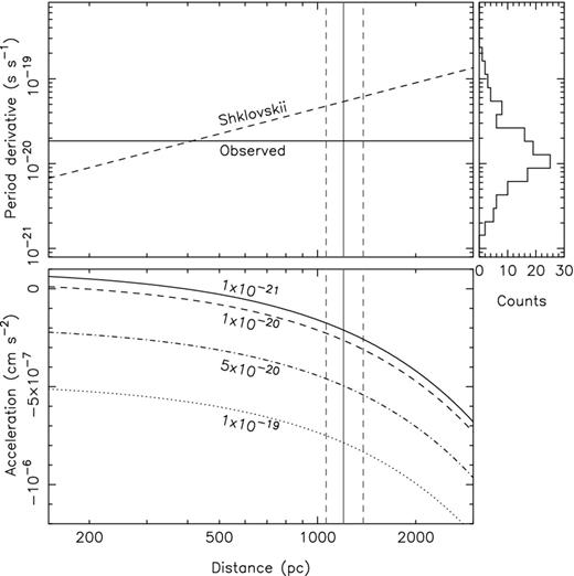
The top panel shows the spin period derivative due to the non-zero proper motion (the Shklovskii effect) as a function of distance as the dashed line. For distances larger than 0.43 kpc, it exceeds the observed spin period derivative (solid horizontal line). The histogram on the right-hand side of the top panel shows the distribution of intrinsic spin period derivatives for all radio millisecond pulsars in the Galactic field (Manchester et al. 2005). The bottom panel shows the radial acceleration required to explain the observed spin period derivative of PSR J1024−0719 given the Shklovskii contribution assuming four different values for the intrinsic spin period derivative of the pulsar. The solid and dashed vertical lines denote the Lutz & Kelker (1973) bias corrected distance of PSR J1024−0719 derived from our parallax measurement.
4.2 Association with PSR J1024−0719
In Table 2, we list the proper motion and pulsar position propagated to the epoch of the OmegaCAM observations (MJD 55984.135) for several timing ephemerides of PSR J1024−0719. Within the uncertainties, the pulsar position and proper motion as measured by the three PTAs are consistent with each other. We find that star B is offset from PSR J1024−0719 by Δα = −0.12(5) arcsec and Δδ = −0.03(4) arcsec, corresponding to a total offset of 0.12(6) arcsec. Here, the uncertainty is dominated by the astrometric calibration against the UCAC4 catalogue. For star F, the total offset is 2.37(11) arcsec. Moreover, the proper motions determined from the 14.2 yr baseline between the FORS1 and FORS2 observations show that, within 2σ, star B has a proper motion consistent with the pulsar.
The similarity in position and proper motion between star B and PSR J1024−0719 is independently confirmed by several surveys. At R = 18.78, star B is bright enough to have been recorded on historic photographic plates and hence is included in the USNO-A2 (Monet et al. 1998) and USNO-B1 (Monet et al. 2003) astrometric catalogues. It is also detected in the near-IR in the 2MASS survey (Cutri et al. 2003; Skrutskie et al. 2006). Star B is present in the PPMXL catalogue by Roeser et al. (2010), which combines the USNO-B1 and 2MASS astrometry to determine proper motions, and also the APOP catalogue by Qi et al. (2015), which uses STScI digitized Schmidt survey plates originally utilized for the creation of the GSC II catalogue (Lasker et al. 2008) to derive absolute proper motions. The position and proper motion of star B in these catalogues is plotted in Figs 3 and 4 and listed in Table 2.
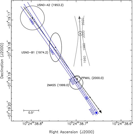
The position of PSR J1024−0719 (black), star B (blue) and star F (grey) between 1950 and 2025. The positional uncertainties of stars B and F are indicated by the ellipses at the OmegaCAM observation of star B (epoch 2012.15) and the FORS1 observation of star F (epoch 2001.24). The lines expanding from the ellipse illustrate the positional uncertainty due to position and proper motion as a function of time. On the scale of this plot, the uncertainties on the timing position and proper motion of PSR J1024−0719 are negligible. Also plotted are measurements of the position of star B in the USNO-A2 (Monet et al. 1998), USNO-B1 (Monet et al. 2003), 2MASS (Cutri et al. 2003; Skrutskie et al. 2006) and PPMXL (Roeser et al. 2010) catalogues. The epochs of these measurements are given in brackets. The USNO-A2 catalogue does not provide positional uncertainties; we conservatively estimate 0.4 arcsec uncertainties on the position.
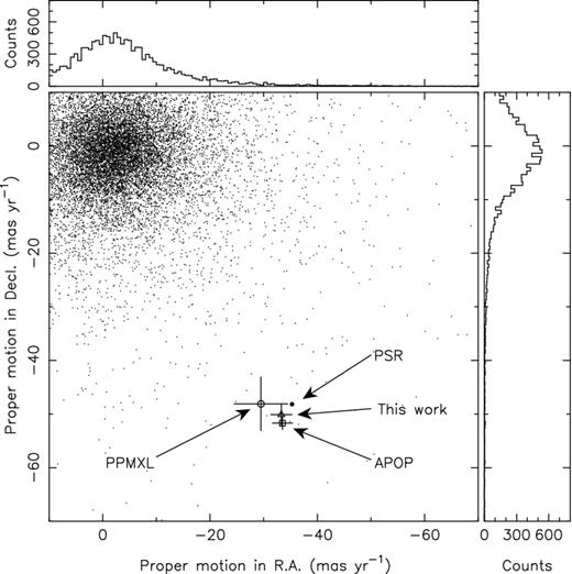
Proper motion measurements of PSR J1024−0719 and star B. The proper motion of PSR J1024−0719 is denoted by the thick black dot. The proper motion of star B as determined in this work, the PPMXL catalogue (Roeser et al. 2010) and the APOP catalogue (Qi et al. 2015) are shown with the triangle, circle and square, respectively. The small points and histograms at the top and right of the figure represent proper motion measurements from stars in the APOP catalogue, selecting 14 754 stars within a radius of |$1^\circ$| around PSR J1024−0719.
The probability that an unrelated star has, within the uncertainties, a position and proper motion consistent with PSR J1024−0719 is minuscule. The APOP catalogue and the FORS2 photometry yield a stellar density for stars with R < 18.78 (equal or brighter than star B) of one to two stars per square arcminute, while within |$1^\circ$| from PSR J1024−0719, only 8 out of 7300 APOP stars with R < 18.78 have a proper motion in right ascension and declination that is within 10 mas yr−1 of that of PSR J1024−0719 (μ = 59.71 mas yr−1). Based on these numbers, we estimate that the chance probability of a star having a similar position and proper motion to PSR J1024−0719 is about 10−7 for stars equal or brighter than star B. Such a low probability confirms that star B is associated with PSR J1024−0719 and that both objects form a common proper motion pair.
At or above the brightness level of star F, there are about 10 objects per square arcminute in the FORS1 R-band image, suggesting that there is a probability of about 7 per cent of finding an object as bright and close as star F with respect to the pulsar position. Hence, we consider star F as a field star, not related to PSR J1024−0719.
4.3 Properties of star B
The spectroscopic observation of star B shows strong absorption lines of Na D and Ca ii, while Hα is weak. There is some suggestion of absorption from the TiO bands near 6300 and 7000 Å. A comparison against templates from the library by Le Borgne et al. (2003) favours a K7V spectral type over K2V or M0V templates. This classification agrees with the previous work by Sutaria et al. (2003), who classified star B as a K-type dwarf.
To obtain the radial velocity and spectral parameters of star B, we compare the observed spectrum (Fig. 5) with synthetic spectral templates from the spectral library of Munari et al. (2005). The templates from this library cover a range in effective temperature Teff, surface gravity log g, rotational velocity vrot sin i and metallicity [M/H]. To account for the resolution of the observed spectrum, we convolved the synthetic spectra with a Moffat profile that has a width equal to the seeing and is truncated at the width of the slit. For each combination of temperature, surface gravity and metallicity, we used the convolved templates to find the best-fitting values for rotational velocity vrot sin i and radial velocity v. These convolved, broadened and shifted spectra were then compared with the observed spectrum while fitting the ratio of observed and normalized flux with a second-order polynomial.
![The FORS2 optical spectrum of star B, formed from the combination of the single exposures obtained with the 600RI and 600z grisms, is shown in black. The spectrum has been shifted to zero velocity. The R- and I-band magnitudes have been converted to fluxes using the zero-points of Bessell, Castelli & Plez (1998) and are plotted. Regions affected by telluric absorption have been masked. The most prominent spectral lines are indicated. Two synthetic spectra by Munari et al. (2005) are shown which bracket the best-fitting model to the observed spectrum. Both model spectra have [M/H] = −1.0 and has been rotationally broadened by 83 km s−1 and convolved by a truncated Moffat profile representing the observational seeing and slit width. The top light-grey model spectrum has Teff = 4250 K and log g = 4.5 cgs, while the dark-grey model spectrum has Teff = 4000 K and log g = 4.0 cgs. The models have been reddened using the extinction law by Cardelli, Clayton & Mathis (1989) and E(B − V) = 0.04 and then scaled to match the observed spectrum. The model spectra are offset by 0.3 and 0.4 vertical units for clarity.](https://oup.silverchair-cdn.com/oup/backfile/Content_public/Journal/mnras/460/2/10.1093_mnras_stw1134/2/m_stw1134fig5.jpeg?Expires=1750291819&Signature=w75fjlrMBt-eN0P37F4g53dV948td4SN3CV4ldfpAetUNNZGE12IgvDzMYzwl7~HOC5~6M9SEAfysUJ1SFP8q64HMXEJXY5sStarUOuzQXirzwTiJmbL1bnq0N5NWhx4e5e~MNnNNv4MJyBLe7vUGjwlOKfWHxNCrzYxw0wx0BA4P8~F4fp9vCQNKfSXK2rA1OVzM3yQX1elNaX3OAK5zLSeFQd3aLPWQZ5gao9qPu~VcPn7~SmJ-fcdxFj8cGhmFcs00iG2n7eK0Duxhqj1yFskxy1wXu4ZQ0du01tGzRUD3fh0uaVwHZvNGuStyVQ1U~iZ453ALUCk91cTbyY8DQ__&Key-Pair-Id=APKAIE5G5CRDK6RD3PGA)
The FORS2 optical spectrum of star B, formed from the combination of the single exposures obtained with the 600RI and 600z grisms, is shown in black. The spectrum has been shifted to zero velocity. The R- and I-band magnitudes have been converted to fluxes using the zero-points of Bessell, Castelli & Plez (1998) and are plotted. Regions affected by telluric absorption have been masked. The most prominent spectral lines are indicated. Two synthetic spectra by Munari et al. (2005) are shown which bracket the best-fitting model to the observed spectrum. Both model spectra have [M/H] = −1.0 and has been rotationally broadened by 83 km s−1 and convolved by a truncated Moffat profile representing the observational seeing and slit width. The top light-grey model spectrum has Teff = 4250 K and log g = 4.5 cgs, while the dark-grey model spectrum has Teff = 4000 K and log g = 4.0 cgs. The models have been reddened using the extinction law by Cardelli, Clayton & Mathis (1989) and E(B − V) = 0.04 and then scaled to match the observed spectrum. The model spectra are offset by 0.3 and 0.4 vertical units for clarity.
To exclude possible pollution of the observed spectrum by telluric absorption, the wavelength ranges between 5600 and 6600 Å and 8400 and 8800 Å were selected for the comparison. These ranges contain the strong lines of the Na D doublet and the Ca ii triplet, but also the weak Hα line. The observed spectrum is best represented by the models with [M/H] = −1.0, at an effective temperature of Teff = 4050(50) K and surface gravity log g = 4.28(19) cgs, broadened by vrot sin i = 83(14) km s−1 at a radial velocity with respect to the Solar-system barycenter of v = 185(4) km s−1. The reduced χ2 = 3.5 for 875 degrees of freedom.
4.4 Mass, distance and reddening
The effective temperature and surface gravity of star B are consistent with those of a low-mass main-sequence star, as higher mass stars will have evolved off the main-sequence and have much lower surface gravities (log g < 3 cgs).
In Fig. 6, we plot the predicted effective temperatures Teff of the PARSEC stellar evolution models of [M/H] = −1.0 by Bressan et al. (2012), Tang et al. (2014) and Chen et al. (2014, 2015) to estimate the mass and distance of star B. Here, we use our Johnson–Cousins VRI photometry as well as the SDSS griz photometry from the ATLAS survey (Shanks et al. 2015), where star B has g = 20.56(2), r = 19.215(10), i = 18.612(15) and z = 18.232(19). We further more use the model by Green et al. (2014, 2015) to obtain the reddening E(B − V) as a function of distance towards PSR J1024−0719. This model predicts that the reddening reaches a maximum value of E(B − V) = 0.040 for distances larger than 800 pc. Combined with the RV = 3.1 extinction coefficients for the VRI and griz filters from Schlafly & Finkbeiner (2011), the observed magnitudes are corrected for absorption and compared with the predicted absolute magnitudes from the PARSEC models to obtain the plotted distance modulus (m − M)0 and hence distance d.
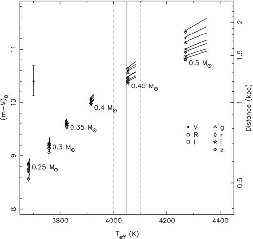
Mass and distance predictions from the PARSEC stellar evolution models by Bressan et al. (2012), Tang et al. (2014) and Chen et al. (2014, 2015) at the observed temperature and broad-band VRI and griz magnitudes. The observed magnitudes were corrected for reddening using E(B − V) = 0.040 from the model by Green et al. (2014, 2015) and the Schlafly & Finkbeiner (2011) extinction coefficients. The error bar on the left denotes the Lutz & Kelker (1973) bias corrected parallax distance of PSR J1024−0719.
We find that models with masses between 0.43 and 0.46 M⊙ can explain the observed temperature. Taking into account the scatter in the distance moduli between the different filters, our dereddened photometry constrains the distance to 1.1–1.4 kpc. These distances are consistent with the parallax distance (corrected for Lutz & Kelker 1973 bias) of |$d=1.20^{+0.18}_{-0.14}$| kpc for PSR J1024−0719 determined from pulsar timing, further confirming the association of star B with PSR J1024−0719.
4.5 Orbit constraints
The question now remains if star B can account for the apparent radial acceleration and higher order spin frequency derivatives seen in the timing of PSR J1024−0719.
Since it is unlikely that star B is in an unbound orbit around PSR J1024−0719, we will consider a bound orbit in the following analysis. In Appendix A, we derive expressions for the line-of-sight acceleration |$\ddot{z}_1$|, jerk |$z_1^{(3)}$|, snap |$z_1^{(4)}$| and crackle |$z_1^{(5)}$| acting on the pulsar due to orbital motion and also show they relate to the spin frequency derivatives. This derivation is similar to that presented in Joshi & Rasio (1997), though we also provide expressions for the projected separation of the binary members on the sky, as our optical and timing astrometry provides an additional constraint.
Besides the line-of-sight acceleration |$\ddot{z}_1$|, the observed second derivative of the spin frequency |$\skew4\ddot{f}$| translates into a jerk of |$z_1^{(3)}=6.1(3)\times 10^{-19}$| cm s−3 along the line of sight. The limits on f(3) and f(4) constrain line-of-sight snap and crackle to |$z_1^{(4)}<4\times 10^{-28}$| cm s−4 and |$z_1^{(5)}<7\times 10^{-36}$| cm s−5, respectively. Furthermore, the angular separation of 0.12 ± 0.06 arcsec between the pulsar and star B at the parallax distance of d = 1.20 ± 0.16 kpc corresponds to a projected separation ρ = 144 ± 75 au.
As shown in Appendix A, six parameters are required to describe the orbit; orbital period Pb, semimajor axis a, inclination i, eccentricity e, argument of perigee ω and true anomaly ν. By treating the companion masses as known, i.e. a pulsar mass of m1 = 1.5 M⊙ and a companion mass of m2 = 0.45 M⊙, we can relate the orbital period Pb to the semimajor axis a, and also to the semimajor axis of the pulsar orbit a1 = a m2/(m1 + m2). To investigate which orbits are allowed by the observations, we performed a Monte Carlo simulation where random values for e, ω and ν were drawn from uniform distributions between 0 ≤ e < 1, |$0^\circ \le \omega <360^\circ$| and |$0^\circ \le \nu <360^\circ$|. Furthermore, we choose random values of |$\ddot{z}_1$| from a uniform distribution between −2 × 10⁻⁷ and −8 × 10⁻⁷ cm s−2 to account for the unknown intrinsic spin period derivative of PSR J1024−0719. These values were used to compute q2 and q3 such that the equations for |$\ddot{z}_1$| and |$z_1^{(3)}$| can then be divided to obtain a1 and sin i. Based on these parameters, values for |$z_1^{(4)}$|, |$z_1^{(5)}$| and ρ were computed and compared with the observational constraints. We consider only those orbits that yield values within 1σ of the observed values or limits.
Fig. 7 shows the results of the Monte Carlo simulation. A total of 10 000 possible orbits are depicted as a function of orbital period. Two families of solutions are found. The solutions with sin i < 0.3 are eccentric (e > 0.2) and have orbital periods up to 2000 yr and favour |$\omega \approx 270^\circ$| and |$\nu \approx 180^\circ$|, i.e. placing the pulsar at apastron and the apsides pointing towards the observer. The second family of solutions is less constrained and allows for essentially all eccentricities, also circular orbits, but requires the orbital period to be longer than 6000 yr and sin i > 0.9. Depending on the eccentricity and orbital period, all values for ν and ω are possible.
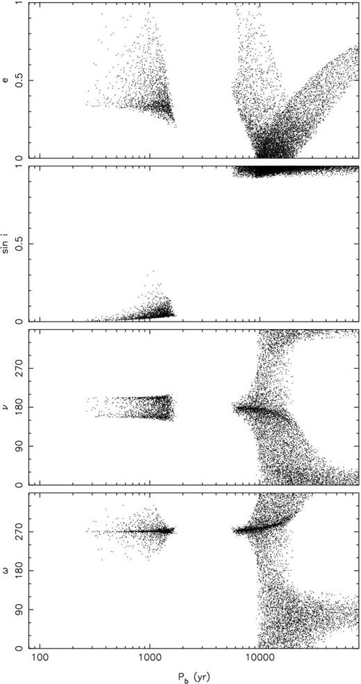
The results of a Monte Carlo simulation to find orbits which account for the observed properties of PSR J1024−0719. Random values for e, ω and ν are drawn from uniform distributions and used to compute Pb and sin i. Only those orbits which predict |$z_1^{(4)}$|, |$z_1^{(5)}$| and ρ consistent with the 1σ measurements or limits are plotted.
4.6 Space velocity
The radial velocity measurement of star B of VR = 185 ± 4 km s−1 complements the transverse velocity VT = 341 ± 45 km s−1 from the proper motion measurement of PSR J1024−0719 and allows us to determine the 3D velocity of the system in the Galaxy. Based on the orbital solutions presented in Section 4.5, we find that the corrections on the transverse velocity of PSR J1024−0719 and the radial velocity of star B with respect to the binary centre of mass are negligible in comparison with the uncertainties on VT and VR. As such, we treat VT and VR as representative of the velocity of the binary centre of mass, yielding a total velocity of 388 ± 39 km s−1 with respect to the Solar-system barycenter. Converting these velocities into the Galactic frame using the algorithm by Johnson & Soderblom (1987)2 and correcting for solar motion with the values from Hogg et al. (2005), the resulting peculiar motion with respect to the local standard of rest is (U, V, W) = (−77, −353, −129) ± (3, 30, 34) km s−1.
The distance, location and proper motion of PSR J1024−0719 place it 0.82 kpc above and moving towards the Galactic plane. Using the MWPotential2014 Galactic potential and the orbit integrator implemented in the galpy software package by Bovy (2015), we numerically integrate the orbit of PSR J1024−0719 in the Galaxy. The result of the integration is plotted in Fig. 8, which shows that the Galactic orbit of PSR J1024−0719 is eccentric and inclined. The Galactic orbit varies between Galactic radii of 4 and 9 kpc (e ∼ 0.5) and reaches up to 5.8 kpc above the Galactic plane. The vertical velocity of the system as it crosses the Galactic plane varies between 120 and 220 km s−1. With these properties, PSR J1024−0719 can be classified as belonging to the Galactic halo (Bland-Hawthorn & Gerhard 2016).
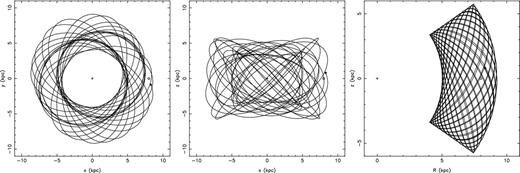
The present Galactic position of PSR J1024−0719 is indicated with the black dot, while the line traces the Galactic orbit of the system over the next 5 Gyr. The location of the Sun at a Galactic radius of R = 8 kpc is denoted with ⊙, while the Galactic Centre is at the plus sign. It is clear that PSR J1024−0719 is in an eccentric and inclined orbit in the Galaxy.
5 A TRIPLE STAR FORMATION SCENARIO
The standard formation scenario for millisecond pulsars is not applicable in the case of PSR J1024−0719. In that scenario, a period of mass and angular momentum transfer from a stellar binary companion spins up an old NS (Alpar et al. 1982; Bhattacharya & van den Heuvel 1991). The outcome of that evolutionary channel is a ‘recycled’ radio millisecond pulsar orbiting the white dwarf remnant of the main-sequence star in a short (0.1 < Pb < 200 d) and circular orbit (e.g. Tauris 2011; Tauris, Langer & Kramer 2012). This channel has been confirmed observationally by the identification of several white dwarf binary companions to MSPs (e.g. van Kerkwijk et al. 2005; Bassa et al. 2006; Antoniadis et al. 2012; Kaplan et al. 2013).
In the case of PSR J1024−0719, the current binary companion is a main-sequence star and thus cannot have recycled the pulsar. Currently, we know of only one other MSP with a main-sequence companion; PSR J1903+0327, which is a 2.15 ms period MSP in a 95 d eccentric (e = 0.44) orbit (Champion et al. 2008) around a 1.0 M⊙ G-dwarf companion (Freire et al. 2011; Khargharia et al. 2012). This system is believed to have evolved from a hierarchical triple consisting of a compact low-mass X-ray binary (LMXB), accompanied by the G dwarf in a wide orbit. The inner companion then was either evaporated by the pulsar (Freire et al. 2011), or the widening of the orbit of the X-ray binary due to mass transfer led to a dynamical instability which ejected the inner companion from the triple (Freire et al. 2011; Portegies Zwart et al. 2011).
For PSR J1024−0719, we argue below that the ejection scenario is unlikely based on its orbital constraints. The evaporation scenario proposed in Freire et al. (2011) is only described qualitatively. To obtain a quantitative description, we investigate if PSR J1024−0719 could have evolved from a triple system in which the inner companion was evaporated. Further considerations of mass transfer, stability, and the effects of supernovae (SNe) in triple systems can be found in Tauris & van den Heuvel (2014).
5.1 Summary of our model
There are a number of criteria which must be fulfilled in order to produce a stable triple system which would eventually leave behind PSR J1024−0719: (i) the triple system must remain bound after the SN explosion which creates the NS, (ii) to survive the SN, the secondary and the tertiary star must therefore be brought close to the exploding star via significant orbital angular momentum loss, e.g. in a common envelope, (iii) the SN explosion must result in a large 3D systemic velocity and cause the tertiary star to be almost (but not quite) ejected, in order to explain the observed properties of PSR J1024−0719, (iv) the post-SN triple system must remain dynamically stable on a long time-scale (i.e. avoid chaotic three-body interactions) and (v) the inner binary must evolve to evaporate the secondary star after the LMXB recycling phase, leaving behind PSR J1024−0719.
We find that the following model is able to account for the criteria listed above, albeit with significant fine-tuning during the SN explosion. The model is illustrated in Fig. 9. Starting on the zero-age main sequence (ZAMS), the system consists of a roughly 16–18 M⊙ primary O-star and two low-mass companions: a secondary F-star with a mass of M2 = 1.1–1.5 M⊙ and a tertiary K-dwarf with a mass M3 ≃ 0.45 M⊙, the presently observed star B (stage 1). After a common envelope phase (stage 2), where the extended envelope of the primary engulfed the other two stars prior to its ejection, the orbital period of the inner binary, Pb, 12 was reduced to a few days and the orbital period of the tertiary star was Pb, 3 ≈ 100 d. Following a phase of wind mass-loss3 from the exposed (initially) ∼6 M⊙ helium core, that star reaches a mass of M1 ≃ 4.3 M⊙ (and Pb, 12 = 3.0 d) when it collapses and undergoes an SN explosion (stage 3). Whereas the inner binary remains compact (but now with a fairly high eccentricity), the dynamical effects of the SN causes the tertiary star to be almost (but not quite) unbound, reaching an orbital period of 102–103 yr in an extremely eccentric orbit (e ≃ 1), and yet remaining in a long-term dynamically stable three-body system (stage 4, see Section 5.3). A combination of tidal damping and magnetic braking eventually causes the secondary star to fill its Roche lobe while still on the main sequence and initiate mass transfer to the NS, i.e. the inner binary becomes an LMXB system (stage 5). The LMXB system is converging, i.e. evolving to a small orbital period, and the secondary star may either form a low-mass helium white dwarf companion with a mass of 0.16–0.20 M⊙ (Istrate, Tauris & Langer 2014) or continue evolving through the period minimum and become a semi-degenerate ‘black widow’-type companion with a mass of a few 0.01 M⊙ (Podsiadlowski, Rappaport & Pfahl 2002; Chen et al. 2013). Meanwhile, the accreting NS is recycled and turns on as an energetic millisecond pulsar which will evaporate its companion star completely (stage 6), thereby leaving behind a system with the presently observed properties of PSR J1024−0719 (stage 7).
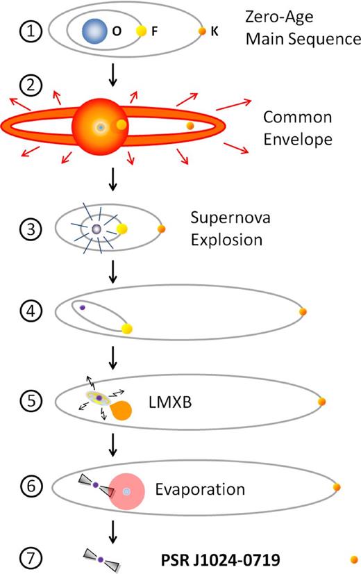
Illustration of the formation of PSR J1024−0719 via a triple star scenario: (1) A triple system is formed with a massive star (an O-star, the progenitor of the NS), an F-star (needed to recycle the NS) and a K-dwarf (star B as presently observed). (2) When the massive star becomes a giant, it expands and engulfs its two orbiting stars. (3) The SN explosion. (4) The dynamically stable post-SN system. (5) Mass-transfer and recycling of the NS during the LMXB phase of the inner binary. (6) Evaporation of the remnant of the secondary star from the energetic wind of the recycled millisecond pulsar. (7) The present-day system PSR J1024−0719. See the text for a discussion of the various stages.
5.2 The dynamical effects of the SN explosion
We now describe in more detail the dynamically important properties of our model. The dynamical effects of asymmetric SNe in binaries, leading to either bound or disrupted systems, has been studied in full detail (Flannery & van den Heuvel 1975; Hills 1983; Tauris & Takens 1998). A general discussion of dynamical effects of asymmetric SNe in hierarchical multiple star systems is found in Pijloo, Caputo & Portegies Zwart (2012), and references therein. Here, we follow their method and apply a two-step process, where we first calculate the effects of an asymmetric SN explosion in the inner binary and then treat the inner binary as an effective point mass with respect to the tertiary star and calculate the dynamical effects of the SN on the outer binary. Hence, we use the obtained recoil velocity of the inner binary as a ‘kick’ velocity added to this effective point-mass star representing the inner binary and then calculate the solution for the outer binary. We assume the SN explosion is instantaneous and for simplicity we neglect in our example any dependence on the orbital phase or inclination of the inner binary with respect to the outer binary.
In the case of a purely symmetric SN (w = 0), a binary will always disrupt if ΔM/M0 > 0.5. This follows from the virial theorem and is also seen when the denominator in equation (1) becomes negative. Since the tertiary star (star B) is almost ejected from the system, we can estimate a critical mass of the exploding star to be 4.55 M⊙ (for which ΔM/M0 = 0.5, if we assume M2 = 1.3 M⊙). In our selected model, we then chose a slightly smaller mass of M1 = 4.3 M⊙ since we also need to apply a kick to obtain a large systemic velocity.
In Fig. 10, we plot examples of the probability4 of the outer binary to remain bound as a function of the resulting recoil velocity, w12 of the inner binary, for three different pre-SN values of the orbital period of the tertiary star (Pb, 3 = 30, 115 and 3000 d). The dots indicate average values of w12 for a given kick velocity added to the newborn NS (between 50 and 350 km s−1). To calculate each of these values, we simulated 107 SN explosions using Monte Carlo techniques. As a result of mass-loss of the inner binary, the minimum value of w12 for any bound solution of the triple system is 67.8 km s−1, thus excluding any solutions in the grey-shaded (forbidden) region in Fig. 10. It is clearly seen that the probability of remaining bound is small for large values of Pb, 3 (e.g. there are no possible solutions if Pb, 3 = 3000 d). The star at w12 = 159 km s−1 is for the selected example investigated further in this scenario (Figs 11 and 12).
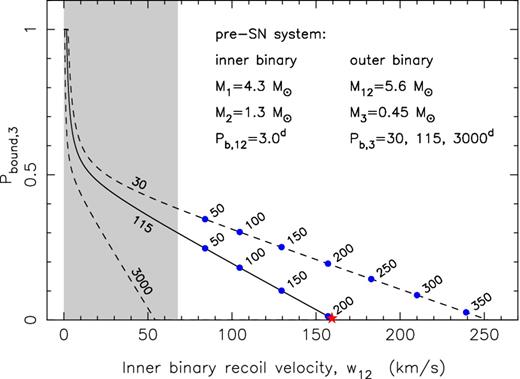
Probability for a triple system to survive a given recoil velocity, w12 obtained by the inner binary due to an SN. The three lines are for a pre-SN orbital period of the tertiary star of Pb, 3 = 30, 115 and 3000 d. The bullet points represent average values of w12 for the stated kick magnitudes (in km s−1) imparted on to the newborn 1.4 M⊙ NS in the inner binary, calculated from Monte Carlo simulation of 107 SNe and using an isotropic distribution of kick directions for both w and w12. When calculating 〈w12〉, only triple systems for which the inner binary avoided merging were considered. However, the long-term stability of the surviving triple systems is not included here. The assumed pre-SN mass of the exploding star is M1 = 4.3 M⊙, the secondary star has a mass of M2 = 1.3 M⊙ and the tertiary star has a mass of M3 = 0.45 M⊙. The pre-SN orbital period of the inner binary is Pb, 12 = 3.0 d. The red star at w12 = 159 km s−1 (Pb, 3 = 115 d) marks the example investigated further in this scenario.
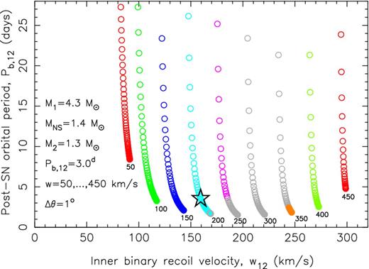
Post-SN orbital period of the inner binary (Pb, 12) as a function of its resulting recoil velocity (w12) and kick velocity (w) imparted on to the NS. Each coloured track is for a given value of w (between 50 and 450 km s−1) and plotted along the tracks are solutions for different values of the kick angle θ (in steps of |$1^\circ$|). Grey circles represent systems that merge during the SN. The open star indicates the selected example which we investigate in more detail.
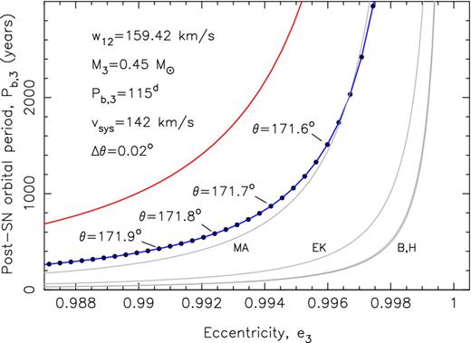
Post-SN orbital period of the tertiary star, Pb, 3 as a function of the eccentricity of its orbit using our selected inner binary model from Fig. 11. The pre-SN model has an orbital period of Pb, 3 = 115 d. Solutions are shown along the blue curve for different values of the kick angle, θ in steps of 0| $_{.}^{\circ}$|02. The grey lines shown minimum orbital periods for a given eccentricity to ensure a long-term stable three-body configuration. The red line shows the expected orbital period after evaporation of the secondary star – see text for discussions.
The values of the pre-SN orbital periods of the tertiary star (Pb, 3) are limited to an interval where it cannot be too large (otherwise the system would dissociate) or too small (in which case the pre-SN triple system would not be stable due to three-body interactions between the stars). Besides reproducing the orbital period of the K-dwarf (star B) in PSR J1024−0719, we must also make sure to reproduce the large systemic velocity, vsys of PSR J1024−0719. As derived in Section 4.6, the vertical velocity of PSR J1024−0719 when it crosses the Galactic plane must be between 120 and 220 km s−1. Hence, our model must produce at leastvsys = 120 km s−1 for an optimal orientation of vsys. A large value of vsys requires a large value of w12, which depends on the magnitude of the kick, w imparted on to the newborn NS during the SN as well as the value of the pre-SN orbital period of the tertiary star Pb, 3.
In Fig. 11, we demonstrate how w12 increases with the kick velocity, w. For these calculations, we assumed in all cases a pre-SN inner binary with circular orbit and M1 = 4.3 M⊙, MNS = 1.4 M⊙, M2 = 1.3 M⊙, Pb, 12 = 3.0 d and varied w between 50 and 450 km s−1 (w = 0 is not included as it would lead to dissociation of the system). Each point (coloured circle) represents a value of the kick angle, θ (in steps of 1|$^\circ$|) for a given value of w. The magnitude of w is given at the bottom of each track which ends at |$\theta = 180^\circ$|. For clarity, we assumed here that the kick was in the pre-SN plane of the inner binary – i.e. the second kick angle |$\phi =0^\circ$| or |$180^\circ$|, where ϕ is the angle between the projection of the kick velocity vector on to a plane perpendicular to the pre-SN velocity vector of the exploding helium star and the pre-SN orbital plane (e.g. fig. 1 in Tauris & Takens 1998). The post-SN orbital period of the inner binary, Pb, 12 is seen to decrease monotonically with larger values of θ, i.e. when the kick is directed backwards compared to the pre-SN orbital motion of the exploding star. Similarly, we have that Pb, 12 → ∞ for θ → θcrit (cf. equation 1). Grey colours mark systems which immediately merge after the SN, i.e. systems where the periastron separation of the post-SN inner binary is smaller than the radius (∼1.1 R⊙) of the secondary star (here assuming a 1.3 M⊙ main-sequence F-star). The secondary star in our model must have a mass between 1.1 and 1.5 M⊙ to be massive enough to evolve within a Hubble time and still be light enough to possess a convective envelope, which is necessary for magnetic braking to operate during the LMXB phase.
The open black star symbol in Fig. 11 indicates our selected example model (see below) for which w = 200 km s−1 and |$\theta =140^\circ$|, leading to post-SN values of Pb, 12 = 3.54 d, e12 = 0.768 and w12 = 159.42 km s−1. The surviving systems for which w = 350–450 km s−1 produce too large post-SN eccentricities to ensure a long-term stable triple system.
As we have seen already in Fig. 10, a pre-SN orbital period of the tertiary star of Pb, 3 = 3000 d (∼8 yr) is much too wide to keep the system bound after the SN explosion. Therefore, the value of Pb, 3 must have been much smaller and in our chosen example Pb, 3 = 115 d. As a result, the eccentricity of the post-SN system must become very large in order for the K-dwarf (star B) to reach post-SN orbital periods of Pb, 3 = 200–1400 yr, as derived in Section 4.5.
In Fig. 12, we plot the post-SN orbital period of the tertiary star, Pb, 3 as a function of the eccentricity of its orbit using our selected inner binary model with w = 200 km s−1 and |$\theta =140^\circ$|, leading to w12 = 159 km s−1, Pb, 12 = 3.54 d and e12 = 0.768 for the post-SN inner binary, and assuming a pre-SN orbital period of the tertiary star of Pb, 3 = 115 d. We only find solutions for a system mimicking PSR J1024−0719 for a very small interval of 171| $_{.}^{\circ}$|6 < θ < 172| $_{.}^{\circ}$|0 given our particular choice of pre-SN parameters. The values of θ are, as expected, close to the critical value of θcrit = 171| $_{.}^{\circ}$|4 where the system dissociates (e3 > 1). We can calculate θcrit for this system from equation (2). The red line indicates the final orbital period of the tertiary star as a consequence of orbital widening when the secondary star has been evaporated (assuming here that the NS has accreted 0.1 M⊙ during the LMXB phase). The final 3D systemic velocity of our model is vsys = 142 km s−1, which is sufficient to explain the Galactic motion of PSR J1024−0719 (Fig. 8). As we discuss below, the post-SN orbit of the tertiary star (star B, the K-dwarf) cannot be too eccentric since this would prevent the post-SN triple system from remaining bound on a long time-scale.
5.3 Long-term stability of a triple system
For all our solutions of bound post-SN triples, we must check if their mutual stellar orbits are dynamically stable on a long-term time-scale. One must keep in mind that it is expected to last several Gyr from the SN explosion until the secondary star evolves through the LMXB phase and finally becomes evaporated. In all this interval of time, the triple system must be stable. This means that for a given eccentricity of the outer binary, we must require that the ratio of the periastron separation of the tertiary star to the semimajor axis of the inner binary, (Rperi/a12) be larger than a critical value. Otherwise, three-body interactions will cause the hierarchical triple to be unstable and eject of one of the stars via tidal disruption or chaotic energy exchange (Mardling & Aarseth 2001). This criterion translates into the requirement that the post-SN orbital period of the tertiary star, Pb, 3, with a given eccentricity, must be larger than a critical value.
Finally, it should be noted that the strict stability criteria of Mardling & Aarseth (2001) was derived for coplanar prograde motion in accordance with a recoil velocity of the inner binary in the orbital plane of the outer orbit. Hence, this criterion represents an upper limit for stability of non-coplanar systems since triple systems whose inner and outer orbits are inclined, despite Kozai interactions (Kozai 1962), will be more stable than coplanar prograde systems with the same mass ratios and eccentricities. Mardling & Aarseth (2001) estimate that for non-coplanar systems, the ratio (Rperi/a12) could be around 30 per cent smaller and still result in long-term stability against escape in the three-body system. This would slightly enhance the probability for producing a system like PSR J1024−0719.
We have demonstrated that PSR J1024−0719 could have formed via a triple system in the Galactic disc. However, estimating the probability for this formation channel would require an investigation combining population synthesis, gravitational dynamics, detailed stellar evolution and hydrodynamical interactions of the common envelope phase, which is much beyond the scope of this paper. While it is difficult to estimate the rate at which binaries like PSR J1024−0719 could be produced from a triple star scenario, we have demonstrated that this scenario is possible, although severe fine-tuning is required for this to happen. Nevertheless, so far we have only detected one such system in our Galaxy.
5.4 Alternative models
A different formation scenario has been suggested by Kaplan et al. (2016). In the scenario, PSR J1024−0719 has been recycled in the centre of a globular cluster, where an exchange encounter with another cluster star or binary led to the ejection of the pulsar from the core of the cluster. In this scenario, the major part of the high space velocity is simply the original velocity of the globular cluster.
The ejection of the inner companion due to a dynamical instability in a triple system, studied in detail by Portegies Zwart et al. (2011) for PSR J1903+0327, does not seem possible for PSR J1024−0719. The reason is that the orbit of the outer companion (the K-dwarf/star B) is expected to harden (i.e. become tighter) if the inner companion is ejected. However, given the current extremely wide orbit, any release of orbital binding energy would have been insufficient to energetically eject the inner companion. The possibility that the ejection event of the inner companion also caused the outer companion to be perturbed into its current extremely wide orbit, from an initially much closer orbit, is not allowed by energy considerations.
Detailed simulations of either the dynamically stable triple evolution scenario presented here, or the globular cluster ejection scenario suggested by Kaplan et al. (2016) will be required to ascertain which scenario is most probable. When better constraints on the orbit of PSR J1024−0719 become available in the future, predictions from these scenarios can be tested.
6 DISCUSSION AND CONCLUSIONS
Since its discovery in 1994, PSR J1024−0719 was thought to be an isolated millisecond pulsar. Our extended EPTA timing ephemeris of the pulsar, combined with optical astrometry, photometry and spectroscopy of the 2MASS J10243869−0719190 (star B), show that PSR J1024−0719 is gravitationally bound to star B, and that the gravitational interaction between the two can account for the apparent discrepancy in the system distance and the steep spectrum timing noise of PSR J1024−0719. We furthermore find that, even though we cannot fully constrain the binary orbit, it must be extremely wide, with orbital periods in excess of 200 yr. A rare formation scenario of PSR J1024−0719 is required to explain the extremely wide binary orbit and the very high space velocity in the Galaxy. We show that PSR J1024−0719 could have evolved from a triple system, though significant fine-tuning during the SN explosion is required.
The binary orbit of PSR J1024−0719 and star B is presently not fully constrained. As a result, the higher order frequency derivatives in the radio timing solution of PSR J1024−0719 will remain free parameters and will hence be a source of timing noise which may limit using PSR J1024−0719 as a PTA source. To fully constrain the orbit by timing PSR J1024−0719 alone, a measurement of five spin frequency derivatives would be required (Joshi & Rasio 1997). Considering the component masses as known, and assuming a value for either |$\dot{P}_\mathrm{int}$| or |$\ddot{z}_1$|, the frequency derivatives would constrain Pb, i, e, ω and ν and provide a description of the timing using the spin frequency and spin frequency derivative as with other pulsars.
Improvements in the timing accuracy of PSR J1024−0719 are expected in future IPTA data releases which combine EPTA, PPTA and NANOGrav observations. The first IPTA data release (Verbiest et al. 2016) contains 15.9 yr of EPTA and PPTA data on PSR J1024−0719. That release contains a subset of the EPTA data used in this paper and hence does not provide stronger constraints than those in Table 1. Combining the timing data presented here with that of NANOgrav (Matthews et al. 2016; Kaplan et al. 2016) and the PPTA (Reardon et al. 2016) should provide an increase in the timing accuracy which, to first order, scales with the square root of the number of TOAs. The uncertainties on the spin frequency derivatives with decrease over time t with tα, where α = −3/2 for f, −5/2 for |$\dot{f}$|, −7/2 for |$\skew4\ddot{f}$| and so on. Hence, the uncertainties on f(3) will already be halved by extending the timing baseline another 4 yr.
Independent astrometry of PSR J1024−0719 will be provided in the near future through an ongoing VLBA pulsar astrometry project (Deller et al. 2011, 2016). The expected uncertainties on position and proper motions will be comparable to that from pulsar timing, while the uncertainty on the pulsar parallax will be significantly better (factor 5–10) compared to the current uncertainty of 0.11 mas on the timing parallax (Deller, private communication).
An improvement in the position and proper motion of star B would also help constrain the orbit through equations (A1) and (A2). Though this would require including the longitude of ascending node Ω as a free parameter, a measurement of differential position and proper motion as well as two spin frequency derivatives would allow a complete description of the orbit. Improving the astrometry presented here through further ground-based observations will be challenging. However, star B is bright enough for its parallax, position and proper motion to be measured by gaia. The photometric transformations by Jordi et al. (2010) estimate a gaiaG-band magnitude of G = 19.1 for its V-band magnitude and V − I colour. The astrometric performance of gaia5 predicts uncertainties on the parallax, position and proper motion of 0.32 mas, 0.23 mas and 0.17 mas yr−1, respectively. These uncertainties are comparable to those of PSR J1024−0719 from the timing solution.
Combining the gaia astrometry of star B with the pulsar timing astrometry of PSR J1024−0719 will provide much stronger constraints on the orbit. For the nominal distance of d = 1.20 kpc, these uncertainties translate to a distance uncertainty of 500 pc, an uncertainty in the projected position on the sky of 0.3 au and a projected velocity uncertainty of 0.9 km s−1. Based on the orbital solutions shown in Fig. 7, the projected velocities on the sky at the nominal distance are in the range of 0.3 to a few km s−1, where the velocity is larger for less eccentric orbits and with the binary members away from apastron, and hence may be measurable from the astrometry of both binary members. This approach will also provide independent constraints on the distance and the intrinsic spin period derivative of PSR J1024−0719.
The full gaia catalogue is expected to be released in 2022. Given the prospect of much tighter constraints on the orbital parameters with this future release, and considering the large pulsar timing data set that has already been accumulated for PSR J1024−0719, we consider it worthwhile to keep observing the pulsar as part of PTAs. Besides contributing to the constraints on nano-hertz gravitational waves, these decade long, multifrequency, pulsar timing data sets like that presented here enable us to measure other effects perturbing the stable rotation of millisecond pulsars and make unexpected discoveries.
We thank David Kaplan for fruitful discussions about the system and the orbital constraints, which helped resolve a mistake in the derivation of the spin frequency derivatives due to orbital motion. This research has made use of the VizieR catalogue access tool, CDS, Strasbourg, France. This research is based on observations made with ESO Telescopes at the La Silla Paranal Observatory under programme ID 95.D-0973(A). Part of this work is based on observations obtained the 100-m telescope of the MPIfR (Max-Planck-Institut für Radioastronomie) at Effelsberg. Pulsar research at Jodrell Bank and access to the Lovell Telescope is supported by a Consolidated Grant from the UK's Science and Technology Facilities Council. The Nançay Radio Observatory is operated by the Paris Observatory, associated with the French Centre National de la Recherche Scientifique (CNRS). The Westerbork Synthesis Radio Telescope is operated by the ASTRON (Netherlands Institute for Radio Astronomy) with support from the Netherlands Foundation for Scientific Research (NWO). The authors acknowledge the support of the colleagues in the EPTA. CGB acknowledges support from the European Research Council under the European Union's Seventh Framework Programme (FP/2007-2013)/ERC Grant Agreement no. 337062 (DRAGNET; PI Jason Hessels). SO is supported by the Alexander von Humboldt Foundation. KL acknowledges the financial support by the European Research Council for the ERC Synergy Grant BlackHoleCam under contract no. 610058. RNC and PL acknowledge the support of the International Max Planck Research School Bonn/Cologne and the Bonn-Cologne Graduate School. GT and IC acknowledge financial support from ‘Programme National de Cosmologie and Galaxies’ (PNCG) of CNRS/INSU, France.
With a rotation matrix for the J2000 input frame.
Given the low metallicity of star B, we only expect a moderate amount of wind mass-loss from the helium star prior to its collapse.
The plotted probabilities do not take into account the specific requirements on the value of the post-SN orbital period of the tertiary star necessary for forming PSR J1024−0719. If including this specific constraint, the probabilities shown would be much lower. Similarly, for estimating the resulting values of w12 we did not filter out those surviving triples which would not survive the SN in long-term stable orbits (see Section 5.3).
REFERENCES
APPENDIX A: SPIN FREQUENCY DERIVATIVES DUE TO ORBITAL MOTION
The time derivatives of z1 translate into time derivatives of the spin frequency f through subsequent derivations of |$\dot{f}=-f \ddot{z}_1/c$|, where c is the speed of light. The derivatives yields |$\ddot{f}=-f z_1^{(3)}/c+\dot{f}^2/f$| and so on. We use the approximation by Joshi & Rasio (1997) by neglecting the higher order terms which tend to be a factor |$\dot{z}/c$| smaller and neglectable. As such, we will use |$\dot{f}=-f \ddot{z}_1/c$|, |$\ddot{f}=-f z_1^{(3)}/c$|, |$f^{(3)}=-f z_1^{(4)}/c$| and |$f^{(4)}=-f z_1^{(5)}/c$|.
