


Abstract
We apply a method recently introduced to the statistical literature to directly estimate the precision matrix from an ensemble of samples drawn from a corresponding Gaussian distribution. Motivated by the observation that cosmological precision matrices are often approximately sparse, the method allows one to exploit this sparsity of the precision matrix to more quickly converge to an asymptotic |$1/\sqrt{N_{\rm sim}}$| rate while simultaneously providing an error model for all of the terms. Such an estimate can be used as the starting point for further regularization efforts which can improve upon the |$1/\sqrt{N_{\rm sim}}$| limit above, and incorporating such additional steps is straightforward within this framework. We demonstrate the technique with toy models and with an example motivated by large-scale structure two-point analysis, showing significant improvements in the rate of convergence. For the large-scale structure example, we find errors on the precision matrix which are factors of 5 smaller than for the sample precision matrix for thousands of simulations or, alternatively, convergence to the same error level with more than an order of magnitude fewer simulations.
1 INTRODUCTION
Frequently in astrophysics and cosmology the final step in any analysis is to compare some summary of the data to the predictions of a theoretical model (or models). In order to make this comparison a model for the statistical errors in the compressed form of the data is required. The most common assumption is that the errors are Gaussian distributed, and the covariance matrix, |$\boldsymbol{\sf C}_{ij}$|, is supplied along with the data. In order for precise and meaningful comparison of theory and observation, the theoretical model, summary statistics derived from the data and |$\boldsymbol{\sf C}_{ij}$| must all be accurately determined. A great deal of work has gone into all three areas.
There are three broad methods for determining such a covariance matrix. First, there may be an analytical or theoretical description of |$\boldsymbol{\sf C}_{ij}$| that can be used (see O'Connell et al. 2015; Grieb et al. 2016; Pearson & Samushia 2016, for some recent examples and further references). Secondly, we may attempt to infer |$\boldsymbol{\sf C}_{ij}$| from the data itself. This is often referred to as an ‘internal error estimate’ and techniques such as jackknife (Tukey 1958) or bootstrap (Efron 1979) are commonly used. Thirdly, we may attempt to infer |$\boldsymbol{\sf C}_{ij}$| by Monte Carlo simulation. This is often referred to as an external error estimate. Combinations of these methods are also used.
Our focus will be on the third case, where the covariance matrix is determined via Monte Carlo simulation. The major limitation of such methods is that the accuracy of the covariance matrix is limited by the number of Monte Carlo samples that are used with the error typically scaling at |$N_{\rm sim}^{-1/2}$| (see e.g. Dodelson & Schneider 2013; Taylor, Joachimi & Kitching 2013; Taylor & Joachimi 2014, for recent discussions in the cosmology context). The sample covariance matrix is a noisy, but unbiased, estimate of the true covariance matrix, while its inverse is both a biased (although correctible) and noisy estimate of the inverse covariance matrix (which we shall refer to as the ‘precision matrix’ from now on and denote by |${\boldsymbol \Psi }$|).
We consider the specific case where the precision matrix is sparse, either exactly or approximately. This may happen even when the covariance matrix is dense, and occurs generically when the correlations in the covariance matrix decay as a power law (or faster). It is worth emphasizing that any likelihood analysis requires the precision matrix, and not the covariance matrix. We present an algorithm that can exploit this sparsity structure of the precision matrix with relatively small numbers of simulations.
The outline of the paper is as follows. In Section 2, we introduce our notation and set up the problem we wish to address. Section 3 introduces the statistical method for entrywise estimation of the precision matrix, plus a series of refinements to the method which improve the convergence. Section 4 presents several numerical experiments which emphasize the issues and behaviour of the algorithm, both for a toy model which illustrates the principles behind the algorithm and for a model based on galaxy large-scale structure analyses. We finish in Section 5 with a discussion of our results, the implications for analysis and directions for future investigation.
2 NOMENCLATURE AND PRELIMINARIES
We will consider p-dimensional observations, |$\boldsymbol x$|, with a covariance matrix |$\boldsymbol{\sf C}$| and its inverse, the precision matrix |${\boldsymbol \Psi }$|; we differ from the usual statistical literature where the covariance and precision matrices are represented by |$\boldsymbol {\Sigma }$| and |$\boldsymbol {\Omega }$| in order to match the usage in cosmology more closely. Since we will need to consider both estimates of these matrices as well as their (unknown) true value, we denote estimates with hats. Individual elements of the matrix are represented by the corresponding lowercase Greek letters, e.g. ψij. We will also want to consider normalized elements of the precision matrix – we will abuse notation here and define these by |$r_{ij} \equiv \psi _{ij}/\sqrt{\psi _{ii} \psi _{jj}}$|.
Summary of notation used in this paper.
| Notation | Description |
|---|---|
| |${\cal N}({\boldsymbol\mu}, \boldsymbol{\sf C})$| | Normal distribution with mean μ, covariance |$\boldsymbol{\sf C}$|. |
| |$x \sim {\cal D}$| | x distributed as |${\cal D}$|. |
| ‖ · ‖F | Frobenius matrix norm (see equation 1). |
| ‖ · ‖2 | Spectral matrix norm (see after equation 1). |
| |${\boldsymbol A}^{\rm t}$| | Transpose of |${\boldsymbol A}$|. |
| k banded | The first k − 1 off-diagonals are non-zero. |
We consider banded matrices in this paper, with different numbers of non-zero off-diagonals. We define a k-banded matrix as one with the main diagonal and k − 1 off-diagonals non-zero.
3 THE METHOD
Our approach in this paper uses the observation that precision matrices in cosmology are often very structured and sparse. Unfortunately, this structure is hard to exploit if computing the precision matrix involves the intermediate step of computing the covariance matrix. Our approach uses a technique, pointed out in Ren et al. (2015), to directly compute the precision matrix from an ensemble of simulations. Unlike that work, which was interested in an arbitrary sparsity pattern, the structure of cosmological precision matrices is expected to be more regular, significantly simplifying the problem.
The steps in our algorithm are as follows.
Estimate the elements of the precision matrix entrywise.
Smooth the precision matrix.
Ensure positive-definiteness of the resulting precision matrix.
Each of these is discussed in detail below. It is worth emphasizing that the key insight here is the first step, and it is easy to imagine variants of the remaining steps that build off an entrywise estimate of the precision matrix.
An immediate question that arises is how one determines that a particular precision matrix is sparse and what the sparsity pattern is. For specific cases, like when is the covariance matrix is known to be Toeplitz (or even approximately so) with decaying off-diagonal elements, an estimate of the sparsity pattern is possible. We do not have a complete answer to this question, but provide a possible ‘data-driven’ solution below. We expect that this will generally require some numerical experimentation.
3.1 Entrywise estimates
The above equation also demonstrates how to make use of the sparsity of the precision matrix. Note that the submatrix |${\boldsymbol \Psi }_{A,A^c}$| (that appears in β) inherits the sparsity of the precision matrix and therefore, one only need regress on a small number of elements of |$Z_{A^c}$|. To illustrate this with a concrete example, consider a tridiagonal |${\boldsymbol \Psi }$| and A = {1}. Equations (4) and (5) imply that Z1 = βZ2 + e where, in this case, β and e are simply scalars, and |$\langle e^2 \rangle = \psi _{1,1}^{-1}$|. Given measurements |$(Z_1^{(1)},Z_2^{(1)},\ldots )$|, |$(Z_1^{(2)},Z_2^{(2)},\ldots )$|, …, |$(Z_1^{(d)},Z_2^{(d)},\ldots )$|, we do an ordinary least-squares fit for β estimating the error e2 and use ψ1, 1 = e−2. The linear regression in this case requires d ≫ 2 observations to robustly determine β and e, compared with d ≫ p observations where p is the rank of the precision matrix; this can translate into a significant reduction in the required number of simulations.
The above is the elementwise distribution of the precision matrix. An extension of these results would be to determine the probability distribution of the entire precision matrix, allowing one to marginalize over the uncertainty in the estimated precision matrix (Sellentin & Heavens 2016). However, as of this work, we do not have such a description of the probability distribution; we therefore defer this possibility to later work.
3.2 Smoothing
We expect the covariance and precision matrices we encounter in cosmology to be relatively ‘smooth’, which we can therefore hope to use to reduce the noise in the entrywise estimates. Such a smoothing operation can take many forms. If we could construct a model for the covariance/precision matrix, one could directly fit the entrywise estimates to the model. For example, on large scales, one might use a Gaussian model with free shot noise parameters (Xu et al. 2012; O'Connell et al. 2015). In the absence of a model, one might use a non-parametric algorithm to smooth the precision matrix, respecting the structure of the matrix. For such an algorithm, the elements of the data vector must be appropriately ordered. In our numerical experiments below, we give an explicit example where we interleave the elements of the monopole and quadrupole correlation functions, which keeps the precision matrix explicitly banded. Different orderings may result in more complicated sparsity patterns, but our algorithm easily generalizes to these cases.
For the examples we consider in this paper, we use a cubic smoothing spline and smooth along the off-diagonals of the matrix, with the degree of smoothing automatically determined by the data using a cross-validation technique. Since we believe that such a smoothing procedure may be generically useful, Appendix C contains an explicit description of the algorithm.
3.3 Maximum-likelihood refinement
The estimate of the precision matrix is ‘close’ to the true precision matrix in a Frobenius sense. However, since the matrix was estimated entrywise, there is no guarantee that |$\boldsymbol{\sf R}_0$| (and therefore |$\hat{\boldsymbol \Psi }$|) is positive definite Our goal in this section is to find a refined estimate |$\boldsymbol{\sf R}$| that is both positive definite and close to |$\boldsymbol{\sf R}_0$|. Since the diagonal matrices |$\boldsymbol{\sf D}$| are positive definite by construction, a positive definite |$\boldsymbol{\sf R}$| guarantees a positive definite |$\hat{\boldsymbol \Psi }= \boldsymbol{\sf DRD}$|.
We perform this optimization using standard techniques; details of the algorithm are in Appendix B.
4 NUMERICAL EXPERIMENTS
4.1 Model covariance and precision matrices
We consider two examples of covariance (and precision) matrices in this paper. First, in order to build intuition, we consider a tridiagonal precision matrix |${\boldsymbol \Psi }= (\psi _{ij})$| where ψii = 2, ψi, i + 1 = ψi − 1, i = −1 and zero otherwise. The structure of the resulting covariance matrix is shown in Fig. 1; unlike the precision matrix, the covariance matrix has long range support. The structure of this precision matrix, and the corresponding covariance matrix, is qualitatively similar to the cosmological examples we will consider later. We fix p = 100; this is similar to the number of parameters in covariance matrices for current surveys.
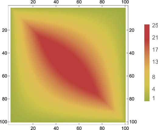
A density plot of the covariance matrix for our toy tridiagonal precision matrix with 2 along the diagonals and −1 on the first off-diagonal.
Secondly, we use an example more closely related to the covariance matrices one might expect in galaxy redshift surveys. Galaxy redshift surveys typically involve negligible measurement uncertainties, but suffer instead from both sampling variance and shot noise. These can be estimated within the framework of a theory, but a theory for the formation of non-linear objects is not currently understood. Instead we use a linear theory approximation. Specifically, we compute the covariance matrix of the multipoles of the correlation function, ξℓ(s), assuming Gaussian fluctuations evolved according to linear theory. The assumed cosmology and power spectrum are of the ΛCDM family, with Ωm = 0.292, h = 0.69, ns = 0.965 and σ8 = 0.8. The objects are assumed to be linearly biased with b = 2 and shot noise is added appropriate for a number density of |$\bar{n}=4\times 10^{-4}\,h^3\,{\rm Mpc}^{-3}$|. We evaluate |$\boldsymbol{\sf C}_{ij}$| in 100 bins, equally spaced in s, for both the monopole and quadrupole moment of the correlation function, interleaved to form a 200 × 200 matrix. Fig. 2 plots the corresponding precision matrix. This is clearly dominated by a narrow-banded structure, and is similar in character to our first case.
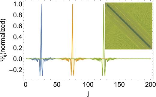
A representation of the precision matrix for the cosmologically motivated example. We plot the 25th, 50th and 75th rows of the matrix, demonstrating that the matrix is clearly diagonally dominant, and very sparse. The inset shows that the full matrix shows the same structure of the individual rows plotted here.
4.2 Entrywise estimates
We start by characterizing the accuracy with which we can estimate individual entries of the precision matrix. As we discussed previously, we separate out the measurements of the diagonal elements of |${\boldsymbol \Psi }$| from the off-diagonal elements; for the latter, we compute |$r_{ij} \equiv \psi _{ij}/\sqrt{\psi _{ii} \psi _{jj}}$|. Figs 3 and 4 show the distributions of the recovered values for two representative entries of the precision matrix of our toy model. The different panels correspond to different numbers of simulations d, while each of the histograms is constructed from an ensemble of 1000 such realizations. We find good agreement with the theoretically expected distributions of both ψii and rij, with the distribution for rij close to the asymptotically expected Gaussian even for relatively small numbers of simulations. All of these results assumed a k = 25 banded structure (i.e. 24 non-zero upper/lower off-diagonals); the results for different choices of this banding parameter are qualitatively similar. Holding the number of simulations d fixed, the scatter in the estimates decreases with decreasing k (the number of assumed non-zero diagonals), since one is regressing on a smaller number of variables in this case.
![Histograms of the recovered values of ψ50,50 for different values of d, correcting for the finite sample bias. We assume that the matrix is banded to k = 25 in all cases. The solid [red] line is the expected distribution of these values.](https://oup.silverchair-cdn.com/oup/backfile/Content_public/Journal/mnras/460/2/10.1093_mnras_stw1042/2/m_stw1042fig3.jpeg?Expires=1750426356&Signature=Fu3B~yqLu6sugp~XVHi8xZBPFydhxJbgBbOOgkOUVczOFGMyS5anxaTwPgwUo3YQPuBYVyr2~0AaSwV0RpLUCvGdUi1TfnTAr1RaHQLF0cMgr2IyscCYeqWg8NUrZpyLGyA6V-TaPpzWrTdddZ9~YcYvaMhXN675qV6DNwO2F~XcNya4CErn-9YFxxk3vFL3JhgDkjiMJzxD9bRswae43YWVjTlp~Q6jBLNz4lfcGRL349ZWdxMmwlnsa4i~olAmx2q~2DPQD-Z3RJStwnFj789E9S-dZikfft~9MEfzmlYSzDE5JBGI5M6eVSE7~b5N7RtJlyrITCkKSrbqaThJ~A__&Key-Pair-Id=APKAIE5G5CRDK6RD3PGA)
Histograms of the recovered values of ψ50,50 for different values of d, correcting for the finite sample bias. We assume that the matrix is banded to k = 25 in all cases. The solid [red] line is the expected distribution of these values.
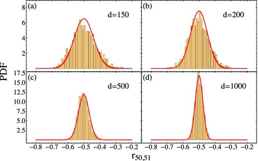
Same as Fig. 3, except for r50,51.
Given these entrywise estimates (each of which will be individually noisy), we turn to the problem of ‘smoothing’ away this noise to improve our covariance estimates. If one had an a priori model for the structure of the precision matrix, one could directly fit to it. For instance, in the case of our toy model, one might use the fact that the matrix has constant off-diagonals. However, in general, one might only expect the matrix to be smooth (nearby entries with the same value); in such a case, using e.g. smoothing splines could provide a reasonably generic solution.
As a worked non-trivial example, we consider smoothing an estimate of our cosmological model. Given that the underlying galaxy correlation function is a smooth function, we would expect the off-diagonals of the precision matrix to be smooth. However, given that our matrix was constructed by interleaving the monopole and quadrupole correlation functions, we would expect this interleaving to persist in the off-diagonals. We therefore smooth the odd and even elements of each off-diagonal separately. Fig. 5 shows the results for two example minor diagonals, comparing it to the raw entrywise estimates as well as the true value. For the majority of the points, smoothing significantly reduces the noise in the entrywise estimates. It can also miss features in the model, if those variations are smaller than the noise. We observe this effect at the edges of the top curves, where the smoothed curves miss the drop-off for the initial and final points. This is clearly a function of the relative sizes of these effects, as is evident from the lower sets of curves where the smoothed estimates track the variations at the edges better.

A demonstration of the impact of smoothing on the elements of the precision matrix for the cosmological model. We plot the odd elements of the first off-diagonal (top, circles) and the even elements of the second off-diagonal for our cosmological model (bottom, squares) (see text for details for how the covariance matrix is packed). The precision matrix was estimated by assuming k = 20 and d = 2000 simulations. The points are the raw entrywise estimates, the dashed line is the true value, while the solid line is the smoothed version. Note that smoothing can significantly reduce the variance of the estimates. More complicated smoothing schemes could reduce the bias at the very edges.
Our final step is to ensure a positive definite precision matrix using the algorithm presented in the previous section. Fig. 6 shows the final results, plotting an example row from the cosmological case. Our estimator tracks the oscillating structure in the precision matrix, and is clearly less noisy than the direct sample precision matrix. This improvement directly translates into improved performance of the precision matrix.
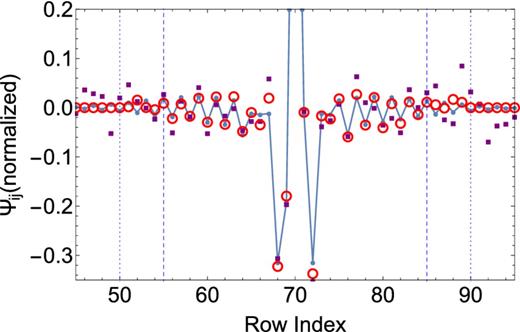
A part of the 70th row of the cosmological precision matrix, normalized by |$\sqrt{\psi _{ii} \psi _{jj}}$|. The filled circles connected by solid lines are the true precision matrix, the filled squares show the sample precision matrix, while the open circles are the estimate developed in this paper. The precision matrix was estimated from d = 1000 simulations, and we assume a banding of k = 20 to estimate the matrix (short dashed lines). The fiducial k = 15 banding that we use for this matrix is marked by the long dashed lines.
4.3 Selecting the banding
We now turn to the problem of determining the banding parameter k. Our goal here is not to be prescriptive, but to develop a simple guide. We anticipate that choosing an appropriate banding will depend on the particular problem as well as some numerical experimentation.
Since we do not expect the off-diagonals of the precision matrix to be exactly zero, choosing a banding reflects a trade-off between bias and variance. By setting small off-diagonals to be zero, our estimated precision matrix will, by construction, be biased. However, any estimate of these off-diagonal elements from a finite number of simulations will be dominated by the noise in the measurements. This also implies that the banding will, in general depend on the number of simulations (except in the case that the matrix is truly sparse); we will see this explicitly in the next section.
We follow a similar procedure for the smoothed estimate of the precision matrix, although the choice of the threshold is complicated by the smoothing procedure and the correlations between different elements on the same off-diagonal. We therefore estimate the threshold by Monte Carlo, simulating m random Gaussian variables, fitting them with a cubic spline and then tabulating the distribution of maximum values. This process ignores the correlations between the points and so, we expect our estimates to only be approximate. Table 2 shows an example of these thresholds as a function of m.
An example of the thresholds at the 95 per cent level for the unsmoothed and smoothed off-diagonals (see text for details on how these are computed). While the thresholds increase for the unsmoothed case, they decrease for the smoothed case since the increase in the number of points better constrain the spline.
| m | Unsmoothed | Smoothed |
|---|---|---|
| 70 | 2.47 | 0.75 |
| 80 | 2.52 | 0.71 |
| 90 | 2.56 | 0.67 |
| 100 | 2.59 | 0.63 |
| m | Unsmoothed | Smoothed |
|---|---|---|
| 70 | 2.47 | 0.75 |
| 80 | 2.52 | 0.71 |
| 90 | 2.56 | 0.67 |
| 100 | 2.59 | 0.63 |
Figs 7 and 8 plot, for a set of simulations, which off-diagonals are determined to be non-zero, using the above criteria. Each row of these figures corresponds to an off-diagonal, whereas each column represents an independent set of simulations from which a precision matrix can be estimated. Since our procedure assumes a banding of the precision matrix, we start by selecting a conservative choice of the band. Filled boxes show off-diagonals that are inconsistent with zero, with the shading representing the confidence level for this. A banded matrix in this figure would appear as a filled set of rows.
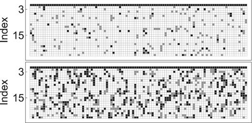
Selecting the banding for the toy model, with each row representing whether a particular off-diagonal was consistent with zero or not. Each row represents an off-diagonal in the scaled precision matrix |${\cal R}$|, with the index of the off-diagonal on the y-axis, while each column represents a set of d = 500 simulations used to estimate the precision matrix. In order to estimate the precision matrix, we assume a banding of k = 25. Unfilled boxes show diagonals consistent with zero, grey boxes show diagonals that are inconsistent with zero at the 95 per cent level but not at 99 per cent, while black represents diagonals inconsistent with zero at the 99 per cent level. An index of one represents the first off-diagonal. The top panel considers the unsmoothed matrix, while the lower panel considers the smoothed case. The tridiagonal nature of the matrix is clearly apparent here, with the first off-diagonal clearly non-zero, and no structure evident for the remaining cases. We choose k = 3 as our fiducial choice for both cases.
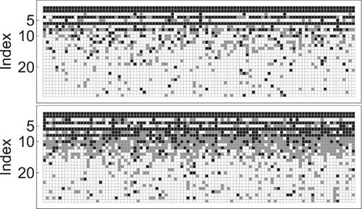
Same as Fig. 7 except for the cosmological model. The number of realizations per column is d = 1000, and the banding assumed for in the estimate is k = 30. The difference between the smoothed and unsmoothed cases is more apparent here. Smoothing requires us to estimate more off-diagonals, due to the reduction in the noise. We choose k = 10 and 15 for the unsmoothed and smoothed cases, respectively.
We start with the unsmoothed cases first (upper panels). The tridiagonal nature of the toy precision matrix is clear, with only a single row clearly visible. The cosmological example is less sharp, but a central band is still clear. The smoothed cases (lower panels) are noisier, because our estimates of the thresholds ignored correlations. Even with this increased noise, we discern no trend suggesting an increased banding for the toy example. For the cosmological example however, the non-zero band is clearly increased, implying that one must work out to a larger band. This is to be expected, since the elements of the precision matrix in this case are not exactly zero. Reducing the noise (by smoothing) reduces the threshold below which one may estimate an element of the precision matrix to be zero. We find a similar trend with increasing numbers of simulations (discussed further below).
A shortcoming of the above is the lack of an objective, automatic determination of the banding. We do not have such a prescription at this time (and it is not clear that such a prescription is possible in general). We therefore advocate some level of numerical experimentation when determining the appropriate band.
4.4 Performance of estimates
We now turn to the performance of our precision matrix estimates as a function of the number of simulations input. There are a number of metrics possible to quantify ‘performance’. The most pragmatic of these would be to propagate the estimates of the precision matrix through parameter fitting, and see how the errors in the precision matrix affect the errors in the parameters of interest. The disadvantage of this approach is that it is problem dependent and therefore hard to generalize. We defer such studies to future work that is focused on particular applications.
A more general approach would be to quantify the ‘closeness’ of our precision matrix estimates to truth, using a ‘loss’ function. There are a variety of ways to do this, each of which test different aspects of the matrix. We consider five such loss functions here:
- Frobenius norm:This is an entrywise test of the elements of the precision matrix, and is our default loss function. Clearly, reducing the Frobenius norm will ultimately improve any estimates derived from the precision matrix, but it is likely not the most efficient way to do so. In the basis where |$\Delta {\boldsymbol \Psi }$| is diagonal, the Frobenius norm is just the RMS of the eigenvalues, and can be used to set a (weak) bound on the error on χ2.(15)\begin{equation} || \Delta {\boldsymbol \Psi }||_{\rm F} \equiv || {\boldsymbol \Psi }- \hat{\boldsymbol \Psi }||_{\rm F}. \end{equation}
- Spectral norm:This measures the largest singular value (maximum absolute eigenvalue) of |$\Delta {\boldsymbol \Psi }$|. This yields a very simple bound on the error in χ2 − |$||\Delta {\boldsymbol \Psi }||_2 |\boldsymbol x|^2$| where x is the difference between the model and the observations.(16)\begin{equation} || \Delta {\boldsymbol \Psi }||_2 \equiv || {\boldsymbol \Psi }- \hat{\boldsymbol \Psi }||_2 \end{equation}
Inverse test: a different test would be to see how well |$\hat{\boldsymbol \Psi }$| approximates the true inverse of |$\boldsymbol{\sf C}$|. A simple measure of this would be to compute |$|| \boldsymbol{\sf C}\hat{\boldsymbol \Psi }- I ||_{\rm F}$| = |$|| \boldsymbol{\sf C}\hat{\boldsymbol \Psi }- \boldsymbol{\sf C}{\boldsymbol \Psi }||$| = |$|| \boldsymbol{\sf C}\Delta {\boldsymbol \Psi }||$|. However, this measure is poorly behaved. In particular, it is not invariant under transposes, although one would expect |$\hat{\boldsymbol \Psi }$| to be an equally good left and right inverse. To solve this, we use the symmetrized version |$||\boldsymbol{\sf C}^{1/2} \hat{\boldsymbol \Psi }\boldsymbol{\sf C}^{1/2} - I||_{\rm F}$|, although for brevity, we continue to denote it by |$||\boldsymbol{\sf C}\Delta {\boldsymbol \Psi }||_{\rm F}$|.
- χ2 variance: given that parameter fits are often done by minimizing a χ2 function, we can aim to minimize the error in this function due to an error in the precision matrix. If we define |$\Delta \chi ^2 = \boldsymbol x^{{\rm t}} \Big ( \Delta {\boldsymbol \Psi }\Big ) \boldsymbol x$|, where as before, |$\boldsymbol x$| is the difference between the data and the model, we define the χ2 loss as the RMS of Δχ2. In order to compute this, we need to specify how |$\boldsymbol x$| is distributed. There are two options here. The first comes from varying the input parameters to the model, while the second comes from the noise in the data. The former is application dependent and we defer specific applications to future work. The second suggests |$\boldsymbol x \sim {\cal N}(0, \boldsymbol{\sf C})$|, in which case we find(17)\begin{equation} \sigma \Big (\Delta \chi ^2\Big ) = \Bigg [ 2 {\rm Tr} \big (\Delta {\boldsymbol \Psi }\boldsymbol{\sf C}\Delta {\boldsymbol \Psi }\boldsymbol{\sf C}\big ) + \big ( {\rm Tr} {\boldsymbol \Psi }\boldsymbol{\sf C}\big )^2 \Bigg ]^{1/2}. \end{equation}
- Kullback–Leibler (KL) divergence: our final loss function is the Kullback–Leibler divergence2 between |$\boldsymbol{\sf C}$| and |${\boldsymbol \Psi }$|, defined byThe Kullback–Leibler divergence can be interpreted as the expectation of the log of the Gaussian likelihood ratio of |$\boldsymbol x$| computed with the estimated and true precision matrices. As in the inverse variance case, we assume |$\boldsymbol x \sim {\cal N}({\boldsymbol{\it 0}}, \boldsymbol{\sf C})$|, which captures the variation in the data.(18)\begin{equation} {\rm KL} \equiv \frac{1}{2} \Bigg [ {\rm Tr} (\boldsymbol{\sf C}{\boldsymbol \Psi }) - {\rm dim}(C) - \log {\,\rm det} (C {\boldsymbol \Psi }) \Bigg ]\,. \end{equation}
Figs 9 and 10 show these different losses for our toy and cosmological models; we plot the ratio of the loss obtained using the sample precision matrix to the loss obtained using the techniques presented in this paper. The figures show the improvement averaged over 50 realizations, although the improvement for individual realizations is similar. For all choices of a loss function, we find that the techniques presented here yield a factor of an ∼few improvement over simply inverting the sample precision matrix. The largest gains come from exploiting the sparsity of the precision matrix and directly estimating it from the simulations. The secondary smoothing step yields a smaller relative (although clear) improvement. Given the similar behaviour of all the loss functions, we focus on the Frobenius norm below for brevity.
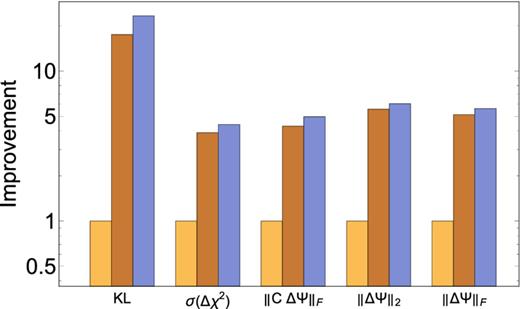
The improvement over the sample precision matrix Loss(sample)/Loss for different norms for the toy tridiagonal precision matrix. From left to right, each group plots the improvement for the sample precision matrix (1 by construction), the unsmoothed and smoothed precision matrices. We assume a k = 3 banding in both the unsmoothed and smoothed cases, and all cases assume d = 500. We average over 50 such realizations in this figure, although the improvements for individual realizations are similar.
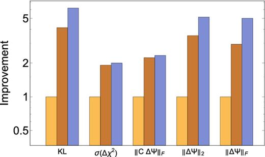
The same as Fig. 9 but for the cosmological model. The unsmoothed covariance matrix assumes k = 10, while the smoothed covariance matrix uses k = 15. All three cases use d = 1000.
We now turn to how the loss depends on the number of simulations d; Figs 11 and 12 summarize these results for both models considered here. The improvements seen above are immediately clear here. At a fixed number of simulations, one obtains a more precise estimate of the precision matrix; conversely, a significantly smaller number of simulations are required to reach a target precision. We also note that we can obtain estimates of the precision matrix with d < p simulations. Given that we assume the precision matrix is sparse, this is not surprising, although we re-emphasize that the usual procedure of first computing a covariance matrix and then inverting it does not easily allow exploiting this property.
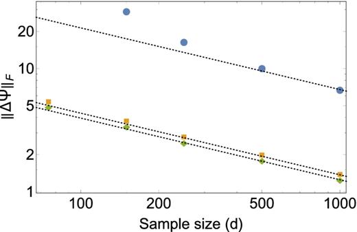
The Frobenius loss |$|| \Delta {\boldsymbol \Psi }||_{\rm F}$| for our toy model as a function of sample size d for the sample precision matrix (blue circles), our estimate of the precision matrix with and without the intermediate smoothing step (green diamonds and orange squares, respectively). The latter two cases assume a banding of k = 3. The dashed lines show a d−1/2 trend which is more quickly attained by the estimates presented in this work than by the sample precision matrix. Recall that this is a 100 × 100 matrix – one cannot estimate the sample precision matrix with d < 100. This restriction is not present for the estimator presented here; all that is required is that d > k.
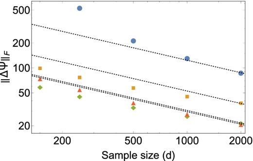
Analogous to Fig. 11 except now for the cosmological model. As in the previous case, the circles (blue) show the sample precision matrix, squares (orange) – our unsmoothed estimate with k = 10, diamonds (green) – our smoothed estimate with k = 15, and triangles (red) – our smoothed estimate with k = 30. Unlike the toy model, we see our estimators flatten out with increasing d at fixed values of k. This reflects the fact that the precision matrix here is not strictly sparse, and that with increasing values of d, one can reliably estimate more elements of the matrix.

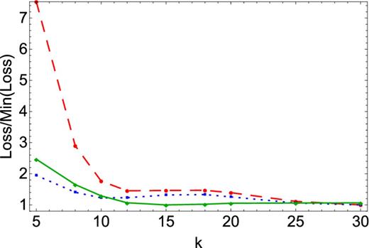
Matrix losses as a function of the choice of the banding parameter k for the toy model. The dashed (red), dotted (blue) and solid (green) lines correspond to the KL, ||CΔΩ|| and ||ΔΩ||F losses, respectively. The losses are all normalized to the minimum value of the loss. Recall that k is defined including the main diagonal (e.g. k = 2 corresponds to one-off diagonal element). All of these are computed for d = 500 simulations. We find a well-defined minimum here, although for two of the three norms, it is at k = 3 and not k = 2.
Same as Fig. 13 but for the cosmological model. The number of simulations used here is d = 1000. Unlike the toy model, there is not a clear optimal banding here, with small changes in the loss for banding k > 10.
Analogous to the fact that the sample precision matrix requires d > p to obtain an estimate, our approach requires d > k to perform the linear regressions. The gains of the method come from the fact that k can be significantly smaller than d.
We can also see how the accuracy in the precision matrix scales with the number of simulations. For d ≫ p, the error scales as d−1/2 as one would expect from simple averaging. However, as d gets to within a factor of a few of p, the error deviates significantly from this scaling; at d < p the error is formally infinite, since the sample covariance matrix is no longer invertible.
The d dependence for our estimator is more involved. For the case of the toy model, we find that the error lies on the d−1/2 scaling for the range of d we consider here, with the smoothed estimator performing ∼10 per cent better. Note that we do not converge faster than d−1/2 – that scaling is set by the fact that we are still averaging over simulations – but the prefactor is significantly smaller. At fixed banding, the cosmological model starts close to a d−1/2 scaling, but then flattens off as d increases. This follows from the fact that the true precision matrix is not strictly zero for the far off-diagonals, and therefore, the error in the estimator has a minimum bound. However, the appropriate banding will be a function of d, since as the number of simulations increases, one will be able to estimate more off-diagonal terms. We see this explicitly in the figure where the k = 30 curve starts to outperform the k = 15 curve at large d.
Motivated by this, we consider how the various losses vary as a function of the assumed banding at fixed number of simulations (see Figs 13 and 14). For the toy model, we find a well-defined minimum k value. Intriguingly, except for the Frobenius norm, it is one larger that the true value. For the cosmological case, the answer is less clear. All the norms suggest k > 10, but have very weak k dependence after that, with possible multiple maxima. This suggests that the particular choice of k will tend to be application specific (and require some numerical experimentation). We defer a more careful study of this to later work.
5 DISCUSSION
This paper describes a method recently introduced in the statistics literature to directly estimate the precision matrix from an ensemble of samples for the case where we have some information about the sparsity structure of this matrix. This allows for getting higher fidelity estimates of the precision matrix with relatively small numbers of samples.
The key result in this paper is the description of an algorithm to directly estimate the precision matrix without going through the intermediate step of computing a sample covariance matrix and then inverting it. It is worth emphasizing that this estimator is completely general and does not rely on the sparsity of the precision matrix. The estimator does allow us to exploit the structure of the precision matrix directly; we then use this property for the specific case where the precision matrix is sparse. However, we anticipate that this algorithm may be useful even beyond the specific cases we consider here.
We also demonstrate the value of regularizing elementwise estimates of the precision matrix. Although this is not the first application of such techniques to precision (and covariance) matrices, we present a concrete implementation using smoothing splines, including how regularizing parameters may be automatically determined from the data.
We demonstrate our algorithm with a series of numerical experiments. The first of these, with an explicitly constructed sparse precision matrix, allows us to both demonstrate and calibrate every aspect of our algorithm. Our second set of experiments uses the covariance/precision matrix for the galaxy two-point correlation function and highlights some of the real world issues that one might encounter, including the fact that the precision matrices may not be exactly sparse. In all cases our method improves over the naive estimation of the sample precision matrix by a significant factor (see e.g. Figs 9 and 10). For almost any measure comparing the estimate to truth we find factors of several improvement, with estimates based on 100 realizations with our method outperforming the sample precision matrix from 2000 realizations (see Figs 11 and 12). The errors in our method still scales as |$N_{\rm sim}^{-1/2}$|, just as for an estimator based on the sample covariance matrix. However, our approach achieves this rate for a smaller number of simulations, and with a significantly smaller prefactor.
A key assumption in our results is that the precision matrix may be well approximated by a banded, sparse matrix. This approximation expresses a trade-off between bias and noise. Banding yields a biased estimate of the precision matrix, but eliminates the noise in the estimate. We present a thresholding procedure to estimate this banding, and find that the width of band increases with increasing sample size, as one would expect. Our banded approximation is similar in spirit to the tapering of the precision matrix proposed by Paz & Sánchez (2015). A hybrid approach may be possible; we defer this to future investigations.
Realistic precision matrices may combine a dominant, approximately sparse component with a subdominant, non-sparse component. For instance, in the case of the correlation function, the non-sparse component can arise even in Gaussian models from fluctuations near the scale of the survey volume, from non-linear effects, as well from the effect of modes outside the survey volume (Harnois-Déraps & Pen 2012; de Putter et al. 2012; Kayo, Takada & Jain 2013; Takada & Hu 2013; Mohammed & Seljak 2014). In these cases, we imagine combining our estimate of the dominant term with an estimate of the non-sparse component (perhaps taken directly from the sample covariance matrix). The key insight here is that our method may be used to estimate the dominant term with higher fidelity. We defer a detailed study of methods for estimating the non-sparse component and combining the estimates to later work.
The computational requirements for the next generation of surveys are in large part driven by simulations for estimating covariance and precision matrices. We present an approach that may significantly reduce the number of simulations required for classes of precision matrices. The ultimate solution to this problem will likely involve combining model-agnostic approaches like the one presented in this work, with improved models for covariance matrices.
We thank the referee, Alan Heavens, for a number of suggestions that improved our presentation of these results. NP thanks Daniel Eisenstein, Andrew Hearin and Uroš Seljak for discussions on covariance matrices. NP and MW thank the Aspen Center for Physics, supported by National Science Foundation grant PHY-1066293, where part of this work was completed. NP is supported in part by DOE DE-SC0008080. HHZ is supported in part by NSF DMS-1507511 and DMS-1209191.
We use d instead of Nsim in what follows for brevity.
A divergence is a generalization of a metric which need not be symmetric or satisfy the triangle inequality. Formally a divergence on a space X is a non-negative function on the Cartesian product space, X × X, which is zero only on the diagonal.
Even though we do not explicitly compute the inverse, there is a substantial cost to solving the linear system.
REFERENCES
APPENDIX A: USEFUL LINEAR ALGEBRA RESULTS
For completeness, we include a few key linear algebra results used in this paper. We refer the reader to Petersen & Pedersen (2012) for a convenient reference.
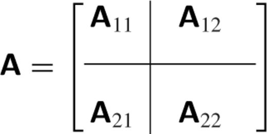
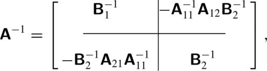
A1 The inverse of a partitioned matrix
A2 Conditional distributions of a multivariate gaussian
APPENDIX B: AN ALGORITHM FOR MAXIMUM-LIKELIHOOD REFINEMENT
Compute the minimization direction v by solving y = Hv.
Compute |$\delta =\sqrt{v^{T} y}$|, and set the step size α = 1 if δ < 1/4; otherwise α = 1/(1 + δ).
Update x → x + αv, and use this to update |$\cal R$| and y. If the update yields an |$\cal R$| that is not positive definite, we backtrack along this direction, reducing α by a factor of 2 each time, until positive definiteness is restored. In practice, this happens rarely, and early in the iteration, and a single backtrack step restores positive definiteness.
The above algorithm is very efficient, converging in ∼50 iterations or fewer for the cases we consider. However, a major computational cost is in inverting the Hessian.3 For a k-banded matrix, s = n(k − 1) − k(k − 1)/2; for some of the cases we consider, this is easily between 103 and 104 elements. Inverting the Hessian every iteration is computationally too expensive, and we transition over to the BFGS algorithm (Nocedal & Wright 2000) for problem sizes s > 1000. Conceptually, the BFGS algorithm (and others of its class) use first derivative information to approximate the Hessian and its inverse. At each step of the iteration, the inverse Hessian is updated using a rank-2 update (equation 6.17 in Nocedal & Wright 2000), based on the change in the parameters and the gradient. Since the algorithm works by directly updating the inverse Hessian, we avoid the computational cost when computing the minimization direction.
We implement algorithm 6.1 of Nocedal & Wright (2000) and refer the reader there for a complete description. We limit ourselves here to highlighting the particular choices we make. The first is the starting approximation to the Hessian; we use the identity matrix for simplicity. While we may get better performance with an improved guess, this choice does not appear to adversely affect convergence and we adopt it for simplicity. The second choice is how to choose the step size in the one-dimensional line minimization. Motivated by our success in the Newton–Raphson case, we use the same step-size choice, with the additional condition that we also backtrack if the error on the previous iteration is <0.9 × the current error. This last condition prevents overshooting the minimum. Note that the Wolfe conditions (Nocedal & Wright 2000) are automatically satisfied with this algorithm due to the convexity of our function.
Finally, we verify that both algorithms converge to the same answer for the same problems.
APPENDIX C: CUBIC SMOOTHING SPLINES AND CROSS-VALIDATION
We summarize the construction of cubic smoothing splines as used here; our treatment here follows (Craven & Wahba 1979, see also Reinsch 1967; de Boor 2001).
Craven & Wahba (1979) suggest a variation on cross-validation to determine the value of p. In ordinary cross-validation, one removes a point at a time from the data and minimizes the squared deviation (over all points) of the spline prediction for the dropped point from its actual value. While conceptually straightforward, actually performing this cross-validation is operationally cumbersome. Craven & Wahba (1979) suggest a weighted variant of ordinary cross-validation (generalized cross-validation), that both theoretically and experimentally, has very similar behaviour, and is straightforward to compute. We outline this method below.
Construct the n × n − 2 tridiagonal matrix |$\boldsymbol{\sf Q}$| with the following non-zero elements qi,i + 1 = qi + 1,1 = 1 and qii = −2, where i = 1, …, n.
Construct the (n − 2) × (n − 2) tridiagonal matrix |$\boldsymbol{\sf T}$| with non-zero elements tn − 2,n − 2 = tii = 4/3 and ti,i + 1 = ti + 1,i = 2/3, with i = 1, …, n − 3.
Compute |$\boldsymbol{\sf F}$| = |$\boldsymbol{\sf QT}$|−1/2. Construct its singular value decomposition |$\boldsymbol{\sf F}$| = |$\boldsymbol{\sf UDV}$|t with |$\boldsymbol{\sf D}$| a diagonal matrix with n − 2 singular values di, and |$\boldsymbol{\sf U}$| and |$\boldsymbol{\sf V}$| being n × (n − 2) and (n − 2) × (n − 2) orthogonal matrices, respectively.
Define the n − 2 values zj by |$\boldsymbol{\sf U}^{t} {\boldsymbol y}$|, where |${\boldsymbol y}$| are the yi arranged in a column vector as above. Define |$\skew3\tilde{d}_i \equiv d_i^2/(d_i^2+p)$|.
- The generalized cross-validation function V(p) is given byWe minimize this function using a simple linear search in log p; the minimum determines the value of p.(C3)\begin{equation} V(p) = \frac{1}{n} \sum _{i=1}^{n-2} \skew3\tilde{d}_i^2 z_i^2 \Bigg / \Bigg ( \sum _{i=1}^{n-2} \skew3\tilde{d}_i \Bigg )^2 \,. \end{equation}
The cubic spline matrix is then given by |$\boldsymbol{\sf I} - {\boldsymbol A} = \boldsymbol{\sf U} {\tilde{\boldsymbol{\sf D}}} \boldsymbol{\sf U}^{{\rm t}}$|, where |${\tilde{\boldsymbol{\sf D}}}$| is an (n − 2) × (n − 2) diagonal matrix with |$\skew3\tilde{d}_i$| on the diagonal.
