


Abstract
We analysed Kepler data of two similar dwarf novae V344 Lyr and V1504 Cyg in order to study optical fast stochastic variability (flickering) by searching for characteristic break frequencies in their power density spectra. Two different stages of activity were analysed separately, i.e. regular outbursts and quiescence. Both systems show similar behaviour during both activity stages. The quiescent power density spectra show a dominant low break frequency which is also present during outburst with a more or less stable value in V344 Lyr while it is slightly higher in V1504 Cyg. The origin of this variability is probably the whole accretion disc. Both outburst power density spectra show additional high-frequency components which we interpret as generated by the rebuilt inner disc that was truncated during quiescence. Moreover, V344 Lyr shows the typical linear rms–flux relation which is strongly deformed by a possible negative superhump variability.
1 INTRODUCTION
Accretion processes are generating a large amount of energy. On sub-galactic scales, accretion occurs in proto- and T Tauri stars and in binary systems where a primary compact object (a white dwarf, a neutron star or a black hole) is accreting matter from a companion star. The class of X-ray binaries contain a neutron star or black hole, where the companion determines whether a systems belongs to the class of low-mass X-ray binaries or high-mass X-ray binaries (see e.g. Lewin & van der Klis 2010 for a review). All accreting binaries in which the central compact object is a white dwarf belong to the class of cataclysmic variables (CVs), where some subclasses derive their definition from the nature of the companion, e.g. red giants in symbiotic systems (see e.g. Marsh 1995; Warner 1995 for a review). Strong magnetic fields can influence the mode of accretion, driving the definition of polars (pure accretion stream), intermediate polars (combination of outer accretion stream and inner accretion disc) and non-magnetic CVs in which an accretion disc is present.
We are interested in a specific subclass of non-magnetic CVs called SU UMa dwarf novae (DN). In general, DN are alternating between quiescence and regular outbursts. The driving mechanism of this alternation is the viscous-thermal disc instability, generated by variations in ionization state of hydrogen (Osaki 1974; Hōshi 1979; Meyer & Meyer-Hofmeister 1981; Lasota 2001). During regular outburst, the mass accretion rate through the disc is high and the disc is fully developed down to the white dwarf surface, while in quiescence the mass accretion rate is much lower and the disc is truncated, i.e. the inner disc region is missing, and evaporated material is forming an inner hot optically thin geometrically thick X-ray corona (Meyer & Meyer-Hofmeister 1994). SU UMa systems show considerably larger superoutbursts that occur in cycles, in addition to the regular outbursts (see e.g. Warner 1995; Lasota 2001 for a review). Two different physical scenarios have been proposed to explain the superoutbursts, i.e. enhanced mass transfer or tidal thermal instability (Schreiber, Hameury & Lasota 2004). The former suggests that the superoutbursts are generated when the disc mass exceeds a critical value, while the latter is based on the outer disc radius expanding to a critical 3:1 resonance radius, where the tidal activity is triggering the superoutburst. Osaki & Kato (2013) analysed the same data as we use in this paper, and concluded that the superoutbursts are initiated by a tidal instability.
Every subclass has its own characteristic physical processes and radiation variabilities, but the driving engine is common, i.e. accretion. Therefore, all systems show fast stochastic variability (so-called flickering) as typical manifestation of the underlying accretion process. This variability is observed over a wide range of energies and time-scales, from infrared to X-rays and from fractions of a second to tens of minutes (see e.g. Bruch 1992). The amplitude of this variability is usually defined as square root of the variance, and a typical linear relation between this variability amplitude and mean flux with lognormal distribution is observed (Uttley, McHardy & Vaughan 2005). This main property of the linear so-called rms–flux relation suggests that the variability is coupled multiplicatively and can be explained by variations in the accretion rate that are produced at different disc radii (Lyubarskii 1997; Kotov, Churazov & Gilfanov 2001; Arévalo & Uttley 2006). The relation is observed in a variety of accreting systems as X-ray binaries or active galactic nuclei (Uttley et al. 2005), CVs (Scaringi et al. 2012a; Van de Sande, Scaringi & Knigge 2015) and symbiotic systems (Zamanov et al. 2015).
Flickering is a red noise process characterized by decreasing power with increasing frequency. Such power law in log–log space (the so-called power density spectrum – PDS) has one or more components separated by characteristic break frequencies (Kato, Ishioka & Uemura 2002; Baptista & Bortoletto 2008; Dobrotka, Mineshige & Ness 2014), after which the red noise slope becomes steeper towards higher frequencies. Long-term observations of a single sky segment available from the Kepler mission offer a unique opportunity to study the PDS in unprecedented detail. Such observational strategy allowed detection of four PDS components in the case of the CV MV Lyr (Scaringi et al. 2012b). An almost continuous light curve of a duration of about 1400 d allowed detailed PDS study during different activity stages of the DN V1504 Cyg (Dobrotka & Ness 2015). Both the outburst and quiescence PDSs of V1504 Cyg show a rather similar high-frequency break, while a lower frequency component is apparently variable between the two activity stages.
V344 Lyr is a DN similar to V1504 Cyg which for a long light curve was observed in the short cadence mode by the Kepler mission. We analyse those data in quiescence and outbursts separately in order to search for the multicomponent nature of the PDSs and the typical linear rms–flux relation. Motivated by the results, we revisit also the V1504 Cyg data in order to search for similarities because both V1504 Cyg and V344 Lyr have similar orbital parameters and belong to the same subclass of SU UMa systems.
2 OBSERVATIONS
The NASA Kepler mission (Borucki et al. 2010) offers a unique opportunity to study fast optical variability of a variety of accreting objects in unprecedented detail, thanks to the high quality of the data: low noise, without any perturbation from the atmosphere and almost continuous1 coverage during long time with a cadence of 58.8 s. This allows detailed studies of the PDSs over a wide frequency range.
As a target of timing analysis we chose two CV systems observed by Kepler, i.e. the SU UMa DN systems V1504 Cyg (KIC number 7446357, orbital period of 1.67 h) and V344 Lyr (KIC number 7659570, orbital2 period of 2.1 h). The light curves of V1504 Cyg/V344 Lyr have durations of approximately 1400 d, and consist of quiescent emission, 118/125 regular outbursts and 11/13 superoutbursts.3 The average quiescent count rates are 448 and 1983 for V344 Lyr and V1504 Cyg, respectively. We are interested in short-term variability during quiescence and regular outbursts.
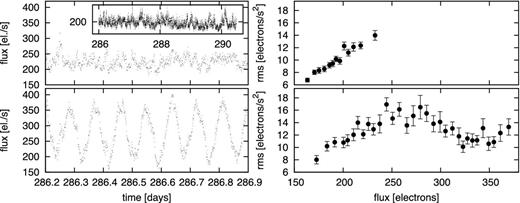
For a quiescent light-curve extraction, we applied two criteria. First, an upper flux limit4 of 1200 electrons/s was used to exclude all outburst data above the limit. Secondly, the times of decline of one outburst and rise into the respective next outburst were determined by a derivative flux limit of 400 electrons/s2. The data in between are the quiescent data. The limits on the derivatives and flux were chosen empirically. Examples of extracted intervals are shown in Fig. 1.
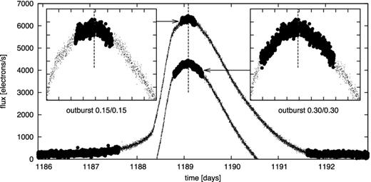
Example of a regular outburst of V344 Lyr. The dots are the original Kepler light curve, and the thick light-curve segments are the selected quiescence and outburst subsamples. Two outburst cases are shown, i.e. 0.15/0.15 and 0.30/0.30 (vertically offset downwards by a value of 2000 for visualization purposes) with details in the inset panels. The moment of outburst maximum (taken as maximum of strongly smoothed light curve) is shown by the dashed line.
The derivative limit method works well for quiescent light curves because the quiescent intervals are long enough and possess high quantity of data, and any border trim does not influence the quality of the resulting PDS. The outbursts are relatively short and the derivative limit method does not work well. Therefore, we adopted an additional method for outburst light-curve extraction. We selected a light curve between some time interval before and after the outburst peak,5 taken from a strongly smoothed light curve. As a smoothing, we selected averaging of n successive light-curve points. Fig. 2 in Cannizzo et al. (2012) suggests that all normal outbursts have a fairly consistent duration, which justifies the use of the same time interval for every outburst. In the subsequent analysis, we denote as ‘outburst 0.10/0.10’ a light curve extracted 0.10 d before and 0.10 d after the outburst peak.

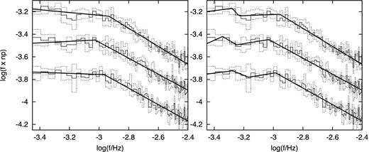
Left-hand and middle panels: quiescent and outburst 0.15/0.15 mean PDSs in different y-axis units. The vertical dashed lines indicate the dominant 2.1 h period with its first harmonic. Right-hand panels: corresponding rms–flux data with error of the mean. The grey data points in the top panel show copied and offset (marked by the arrow) data marked by the shaded area. See the text for details.
3 TIMING ANALYSIS
3.1 Method
For the PDS calculation, we used the Lomb–Scargle algorithm (Scargle 1982) which can handle gaps in the light curves or non-equidistant data. The low-frequency end of the studied PDSs usually depends on the light-curve duration. The high-frequency end is usually limited by white noise or the power rising to the Nyquist frequency, and we empirically defined this limit to log(f/Hz) = −2.2.6 The quiescent data were divided into 1 d intervals, yielding the low-frequency limit approximately log(f/Hz) = −5.0, and every quiescent interval yields an individual PDS. The outburst light curves are too short for further division; therefore, we determine a PDS for each full outburst light curve. A mean PDS was calculated from all individual PDSs. We subsequently binned the mean PDS and a mean value with the standard deviation as an indicator of the intrinsic scatter (error estimate) within each averaged frequency bin was calculated from all points in the bin. We used constant number of mean PDS points with a frequency step of log(f/Hz) = −5.0 for every bin to get consistent PDS estimate. This number was chosen empirically (equal to 5) in order to get acceptable signal-to-noise ratio.
Two y-axis units are commonly used by authors, i.e. a power7np or frequency multiplied by the power f × np. In np units, the white noise is a constant, while it is an increasing power law in f × np units. Furthermore, any red noise is a decreasing power law in np units, while it can be an increasing power law in f × np units in the case of shallow red noise. Therefore, for visualization purposes, we first use np units, but for subsequent detailed analysis we use f × np as y-axis units.
All resulting binned PDSs were fitted with individual multicomponent8 models using gnuplot9 software, yielding searched break frequencies with standard errors calculated from the variance-covariance matrix directly by the fitting software.
3.2 V344 Lyr
3.2.1 PDS analysis
The mean PDSs of V344 Lyr calculated from quiescent and outburst data (0.15/0.15 case) in both y-axis units are shown in the left-hand and middle panel of Fig. 2. While the middle panel can suggest that the PDS is dominated by the Poissonian noise, the left-hand panel with different y-axis units proves that the variability is a red noise. The difference is due to very low slope of the red noise. Furthermore, the dominant period of 2.1 h is clear and is marked, together with its first harmonic, by vertical dashed lines. Both PDSs show an obvious break frequency around log(f/Hz) = −3.45. The low-frequency part of the outburst PDS is rising because of a long-term trend typical for every outburst. Therefore, for direct comparison of both activity stages, we concentrated our study at frequencies above log(f/Hz) = −3.8.
Detailed and binned PDS from the quiescence is shown in Fig. 3. The dominant low break frequency is clear. Using the two-, three- and four-component models yields |$\chi ^2_{\rm red}$| of 1.63, 1.18 and 1.20, respectively. We conservatively assume the scatter within each bin of the averaged PDS to correspond to the statistical errors. The additional break frequency in the best three-component models is not the break frequency we are interested in, because the power increases towards higher frequencies after this break. This is a standard shape when red noise is losing steepness before changing to white noise.

Binned mean PDSs examples of V344 Lyr for both activity stages with multicomponent fits. Two best outburst cases are shown, i.e. outburst 0.15/0.15 and 0.15/0.20. The latter is shifted vertically by 0.3, while the quiescent PDS by 0.8 for visualization purposes.
The |$\chi ^2_{\rm red}$| from different model fitting of various outburst PDSs are summarized in Table 1. Apparently the shorter the light curve, the poorer the fit. This is not surprising as shorter data sets yield larger PDS scatter and not only the errors are larger, but also any real PDS features are buried in the noise. First, we concentrated the fitting to the four-component model. It yields better solutions almost in all cases, at least in those with smallest |$\chi ^2_{\rm red}$|. Just in one case, the four-component model did not converge properly. The higher break frequency is even visually non-identifiable in this case. A visual inspection suggests another ‘peak’ at approximately log(f/Hz) = −2.8. Therefore, additional six-component fit was performed with even better |$\chi ^2_{\rm red}$| (summarized in Table 1). Two best models with six-component fits are depicted in Fig. 3. Larger extraction limits yielding longer outburst light curves started to lose the higher break frequency because the light curve started to extend too far to the rising or declining branch of the outburst (outburst 0.30/0.30 in Fig. 1).
|$\chi ^2_{\rm red}$| values from two- (2 pl) and four-component (4 pl) fits for various outburst light curves (lc) for V344 Lyr (lyr) and V1504 Cyg (cyg).
| Outburst lc | |$\chi ^2_{\rm red}$| | |$\chi ^2_{\rm red}$| | |$\chi ^2_{\rm red}$| | |$\chi ^2_{\rm red}$| | |$\chi ^2_{\rm red}$| | lc duration |
|---|---|---|---|---|---|---|
| 2 pl | 4 pl | 6 pl | 2 pl | 4 pl | (d) | |
| lyr | lyr | lyr | cyg | cyg | ||
| 0.15/0.20 | 1.70 | 1.37 | 1.26 | 0.76 | 0.77 | 0.35 |
| 0.10/0.20 | 2.73 | 2.36 | 2.22 | 0.92 | 0.94 | 0.30 |
| 0.15/0.15 | 1.27 | 1.20 | 1.09 | 1.08 | 1.08 | 0.30 |
| 0.15/0.10 | 5.19 | 3.73 | 3.33 | 1.74 | 1.69 | 0.25 |
| 0.10/0.15 | 2.39 | 2.31 | 2.24 | 1.93 | 2.01 | 0.25 |
| 0.10/0.10 | 3.25 | – | 2.95 | 2.26 | 2.39 | 0.20 |
| 0.15/0.05 | 4.44 | 4.49 | 3.04 | 5.47 | 5.51 | 0.20 |
| 0.10/0.05 | 5.44 | 5.51 | 5.15 | 4.76 | 3.96 | 0.15 |
Finally, based on best fits, we summarize the resulting break frequencies with standard errors in Table 2.
PDS parameters with errors. ‘npl’ means number of power laws used in the fitted model and ‘dof’ means degree of freedom.
| Binary | PDS | log(flower/Hz) | log(fhigher,1/Hz) | log(fhigher,2/Hz) | |$\chi ^2_{\rm red}$| | npl | dof |
|---|---|---|---|---|---|---|---|
| V344 Lyr | quiescence | −3.43 ± 0.01 | – | – | 1.18 | 3 | 117 |
| V344 Lyr | outb. 0.15/0.15 | −3.46 ± 0.13 | −3.02 ± 0.03 | −2.81 ± 0.03 | 1.09 | 6 | 111 |
| V1504 Cyg | outb. 0.10/0.20 | – | −2.97 ± 0.03 | 0.92 | 2 | 69 | |
| V1504 Cyg | outb. 0.10/0.20 | −3.28 ± 0.11 | −2.99 ± 0.04 | 0.94 | 4 | 65 | |
| V1504 Cyg | outb. 0.15/0.15 | – | −3.03 ± 0.02 | 1.08 | 2 | 69 | |
| V1504 Cyg | outb. 0.15/0.15 | −3.34 ± 0.07 | −3.03 ± 0.03 | – | 1.08 | 4 | 65 |
| V1504 Cyga | outb. 0.15/0.20 | −3.34 ± 0.03 | −3.02 ± 0.04 | −2.87 ± 0.03 | 1.03 | 5 | 9 |
| V1504 Cygb | quiescence | −3.38 ± 0.01 | – |
3.2.2 Rms–flux
The rms–flux relations of both stages are depicted in the right-hand panels of Fig. 2. The outburst case behaviour is not surprising when compared to V1504 Cyg (Dobrotka & Ness 2015), but the quiescent case is a surprise. There is a tendency for two linear trends separated by a noisy/variable plateau approximately between flux of 320 and 470 electrons. The high-flux tail is totally non-standard, i.e. decreasing rms with the increasing flux. The last data point suggests a possible inversion of the trend.
3.3 V1504 Cyg
The V344 Lyr finding in the previous section motivated us to reanalyse the data of V1504 Cyg, in order to test whether the low frequency in V1504 Cyg PDS is really significantly different between the activity stages as presented in Dobrotka & Ness (2015), or the quiescent signal at log(f/Hz) = −3.38 is hidden and non-detected in the outburst PDS noise in Dobrotka & Ness (2015).
We followed the same analysis procedure as in V344 Lyr case described in Section 3.1, while for the low-frequency PDS end we used empirically chosen value of log(f/Hz) = −3.45, because we are interested in the same frequencies as studied in Dobrotka & Ness (2015), i.e. higher than the first harmonic of the orbital frequency. We tried again more outburst variants and fitted models. The situation is not that clear as in V344 Lyr analysis, i.e. the four-component model does not give clearly better |$\chi ^2_{\rm red}$|, but neither significantly worse. In Table 1, we summarize all |$\chi ^2_{\rm red}$| from individual fitted models. Apparently, the shorter the light curve, the poorer the fit as already seen in V344 Lyr. Another remark is the |$\chi ^2_{\rm red}$| difference between two- and four-component models for best fits with |$\chi ^2_{\rm red}$| close to 1; they do not differ significantly or are even equal. Therefore, we cannot definitely conclude whether the lower break frequency seen in quiescence is a real PDS feature, neither to rule it out. Fig. 4 shows the three best cases with both two- and four-component fits, and the fitted break frequencies from models with |$\chi ^2_{\rm red}$| closest to 1 are summarized in Table 2.
V1504 Cyg outburst (from top to bottom) 0.15/0.20, 0.15/0.15 and 0.10/0.20 PDSs (thin solid line) with estimated errors (dotted line). The thick solid line is the fitted two- (left-hand panel) and four-component (right-hand panel) model.
3.4 PDS binning
In order to test the reality of detected PDS features, we performed an additional analysis of the best PDSs with frequency binning and error estimate as in Dobrotka & Ness (2015). Instead of a constant-frequency step, we used a constant logarithmic interval in frequency, and instead of the standard deviation we used error of the mean. The former better describes the intrinsic scatter of the binned mean PDS, while the latter better represents the scatter of the binned points.
The V344 Lyr case with mean PDS binned into 0.1 dex in the logarithmic frequency scale is depicted in the left-hand panel of Fig. 5 (outburst 0.15/0.15). The PDS shape is well visible with minimal noise and the four-component nature is unambiguous. Two- and three-component fits yield unacceptable |$\chi ^2_{\rm red}$| of 4.36 and 2.73, respectively, while the four-component model yields a value of 1.30. However, this binning version cleans up the ‘peak’ at log(f/Hz) = −2.81, and a smaller frequency step is required. A binning of 0.05 dex yields larger data scatter, which negates the meaning of this binning version, and the resulting |$\chi ^2_{\rm red}$| are not acceptable for any model. However, once the initial parameters are set up, the optimization method converges and finds a peak around log(f/Hz) = −2.81, but with a doubtful shape and with unconstrained PDS parameters errors,10 probably because of low data points to fit (degree of freedom). Therefore, this binning version is not adequate for a quantitative study of the V344 Lyr PDS.
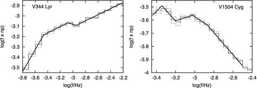
Binned best mean PDSs with different binning procedure than used previously. The errors are the errors of the mean, instead of the standard deviation (see the text for details). Left-hand panel: best V344 Lyr outburst 0.15/0.15 case with a four-component fit. Right-hand panel: best V1504 Cyg outburst 0.15/0.20 case with a five-component fit.
Another situation appears in the case of V1504 Cyg, with mean PDS binned into 0.05 dex (outburst 0.15/0.20, right-hand panel of Fig. 5). The multicomponent shape is again unambiguous with a four-component model yielding a |$\chi ^2_{\rm red}$| of 1.35. Visual inspection suggests that an additional break frequency is present above the main break at log(f/Hz) = −3.0. Therefore, we fitted the data with a five-component model and we got a |$\chi ^2_{\rm red}$| of 1.03. The resulting break frequencies are summarized in Table 2. This finding suggests that the outburst light-curve selection method used in this paper is better than the one used in Dobrotka & Ness (2015), where we used the same data, binning and error estimate.
4 DISCUSSION
4.1 PDS analysis
We analysed Kepler data of two similar DN V344 Lyr and V1504 Cyg in order to search for characteristic break frequencies in PDS from different activity stages, i.e. regular outbursts and quiescence. The analysis of V344 Lyr is new, while the V1504 Cyg data were already analysed for this purpose but differently in Dobrotka & Ness (2015) yielding different low-frequency PDS ends between outbursts and quiescence which we do not find for V344 Lyr. Such significantly different behaviour of such similar systems is unlikely, which motivated us to reanalyse the V1504 Cyg data.
4.1.1 PDS break frequencies
Using different y-axis units and different outburst light-curve extraction limits, we can conclude that quiescent and outburst PDSs of V344 Lyr show a dominant break frequency at log(f/Hz) = −3.4, and two additional break frequencies are present during outburst at log(f/Hz) = −3.02 and −2.81.
V1504 Cyg data yield similar results for the low-frequency break at log(f/Hz) = −3.3 during outburst, which agrees within the estimated errors with a value of log(f/Hz) = −3.38 present during quiescence detected by Dobrotka & Ness (2015). The higher break frequency, previously thought as a modified log(f/Hz) = −3.38 quiescent break frequency, is clear at log(f/Hz) = −3.0 as already detected in outburst by Dobrotka & Ness (2015). Furthermore, an additional break frequency at log(f/Hz) = −2.87 is present during the outburst.
Therefore, both similar systems do show a similar behaviour with a low frequency present during quiescence and an additional PDS complex consisting of two higher break frequencies during outburst. The only significant difference between both systems is the red noise slope which is much shallower in V344 Lyr. This is shown in Fig. 6 where the PDS fits in both stages are compared.
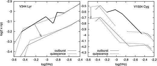
Comparison of quiescent and outburst PDS fits of V344 Lyr (left-hand panel) and V1504 Cyg (right-hand panel). The upper PDSs with thick lines are the fits from Figs 3 (outburst 0.15/0.15) and 4 (outburst 0.10/0.20). The V1504 Cyg fit is expanded by two additional power laws to reach also the high-frequency part for direct comparison with quiescent fits taken from fig. 2 of Dobrotka & Ness (2015). The quiescent fits are shifted vertically by −0.10 for V344 Lyr and −0.22 for V1504 Cyg to be better comparable with the outburst PDSs. The thick line represents the additional outburst component not detected in quiescence. The lower PDSs are the same but shifted (marked by the arrow) for visualization purposes, and with the thick lines removed to show the similarity of both PDS fits without the additional outburst component.
The V344 Lyr case is shown in the left-hand panel. The slopes below the lower break frequency are different between quiescence and outburst which is expected because of long-term trend causing shallower slope in outburst (Fig. 2). The high-frequency ends of both fits have similar slopes. The only significant difference is the PDS pattern characterized by two break frequencies at log(f/Hz) = −3.02 and −2.81 in outburst. This appears like additional components are present in the outburst PDS (marked as thick line) compared to the quiescent case. Otherwise both fits/PDSs have very similar behaviour, which is shown by the shifted PDS (for better comparison) fits where we artificially excluded the additional outburst component.11
The V1504 Cyg case is depicted in the right-hand panel of Fig. 6. We used quiescent PDS fits from Dobrotka & Ness (2015) and expanded the outburst fit derived in this paper to higher frequencies by adding two more power laws in order to be better comparable with quiescence. The additional outburst PDS components are again marked with thick lines, and removed12 from the offset PDS for direct comparison with the original one.
This suggests that the quiescent flickering sources remain radiating during the outburst, and an additional flickering source/sources is/are emerging or becoming more pronounced (not detectable during the quiescence) during the outburst.
4.2 Rms–flux analysis
In the outburst rms–flux relation of V344 Lyr, we can definitely rule out the typical linearity of the relation as expected from the similar system V1504 Cyg (Dobrotka & Ness 2015). The quiescent case is too complicated to confirm or rule out the typical linear relation. Two linear trends marked as shaded areas in Fig. 2 are clear. The light curve of V344 Lyr shows a strong signal around 2.1 h, which may be the orbital period, although following Still et al. (2010) this signal can also be a negative superhump generated by the retrograde-precessing accretion disc. Such superhumps can deform the otherwise present linear rms–flux relation by adding some flux offset proportional to the superhump amplitude. This scenario is marked by the arrow in Fig. 2, i.e. removing the rms plateau between the flux of 320 and 470 electrons, we get the searched linear relation. The grey data points are a copy of the data in the right shaded area and offset horizontally by a flux of 165. We estimated this offset visually and it agrees well with a mean amplitude of the quiescent variability depicted in fig. 1 in Still et al. (2010). Therefore, the rms–flux relation of V344 Lyr can still have the typical linear shape, but is somehow deformed due to other variability sources not connected with the accretion process or flickering.
Upper-left panel: a V1504 Cyg light-curve sequence (all in the inset panel and details in the main panel). Lower-left panel: the same as the upper panel but with added sinusoidal variability. Right-hand panels: corresponding rms–flux data with errors of the mean.
The real light curve is rather complicated; hence, we tried an additional modification. Following Still et al. (2010), the superhump variability is not present during whole quiescence. Therefore, the signal is variable and parameters like amplitude can vary or even disappear. We performed the same approach with artificial superhumps, but we divided the light curve into two parts. One is superhumping as in the previous case, while the second half is not. We did not observe any change. Subsequently, we tried a variable superhump amplitude with a half amplitude superhump for the second light-curve part. The result is depicted in Fig. 8, where we compare the original observed rms–flux data from Fig. 2 with the simulated ones. The original V344 Lyr data were modified horizontally and vertically for direct comparison. Clearly, the behaviour of both is very similar with both rising linear parts, rms plateau and the final decreasing trend with a possible trend inversion at the end. Therefore, we can conclude that V344 Lyr has the typical linear rms–flux relation, but might be considerably deformed by superhumping variability with variable amplitude.

Comparison of observed and ‘simulated’ rms–flux data for V344 Lyr. The data points are calculated from a modified (see the text for details) segment of V1504 Lyr light curve, which exhibits the linear rms–flux relation. The line is the observed rms–flux data from the bottom-right panel of Fig. 2 modified horizontally and vertically in order to match the points for direct comparison.
4.3 Final model
In this study, we are mainly interested in the difference between quiescence and outburst, because it is well known what is the main difference in DN, i.e. a truncated versus fully developed accretion disc (see e.g. Lasota 2001 for a review). Both studied systems show a low-frequency break during quiescence which remains present during outburst with the same of slightly higher value. This component should be generated by a structure which is present in both activity stages and is not changing dramatically. The additional and perhaps dominant (in V1504 Cyg) component is present only during outburst, which suggests that the source is a structure formed during the outburst. Such structure can be the inner disc which is truncated during quiescence. Therefore, we suggest a model, where an accretion disc during quiescence is generating the low-frequency break, while it remains present during outburst and the rebuilt inner disc is somehow much more turbulent generating an additional component with a higher break frequency value.
Why should the inner disc be more turbulent than the preexisting truncated disc? The explanation is the Kelvin–Helmholtz instability, occurring whenever there is a velocity gradient to the flow along the direction that separates two fluids. The geometrically thin disc is rotating with a different radial velocity than the inner hot corona surrounding it, which is the source of the mentioned velocity gradient satisfying condition for enhanced turbulence generation of the disc–corona boundary via Kelvin–Helmholtz instability. It is believed that during quiescence, the corona is formed by evaporation of inner disc material because of inefficient cooling in the low mass accretion rate regime. But it appears that this hot structure is not only present during quiescence. Following Scaringi (2014), the highest break frequency of MV Lyr in PDS calculated from Kepler data is generated by this geometrically thick corona (the so-called sandwiched model) which is confirmed by XMM–Newton X-ray observations (Dobrotka et al., in preparation).
The Kelvin–Helmholtz instability as turbulence generator below the corona as a dominant fast variability source is an attractive scenario to explain also the hybrid rms–flux relation observed during outburst in both studied systems. The rms–flux linearity is an imprint of the multiplicative accretion process where variabilities from different disc rings have characteristic time-scales and are correlated, i.e. the mass accretion rate fluctuation at outer disc radii influences the mass accretion rate variability at innermost disc ring. If Kelvin–Helmholtz instability generates turbulences, these appear chaotically and a corresponding mass accretion rate at a certain radius is then not necessarily correlated to a farther-out fluctuation. Therefore, the fast variability generated by the disc satisfying the linear rms–flux relations is complemented by another variability with a different behaviour. Dobrotka & Ness (2015) showed that an additional ‘constant’ source deforming the linear rms–flux relation is at work during outburst. It is beyond the scope of this paper to investigate whether the variability generated by Kelvin–Helmholtz instability satisfies this condition.13
The proposed final model is depicted in Fig. 9 together with the inner hot corona as a possible source of an additional high-frequency component of V1504 Cyg between log(f/Hz) = −2.3 and −2.4 detected in Dobrotka & Ness (2015).
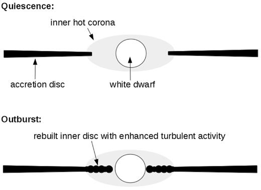
A model of the situation generating a different PDS in quiescence and outburst. See the text for details.
Having found two characteristic break frequencies in the outburst PDS of both SU UMa systems suggests that the emission from the outburst does not originate from a single structure. More detailed investigations of structures are beyond the scope of this study.
The main difference between the two systems is the very different slope of the red noise. While more detailed studies of the red noise are beyond the scope of this work, we find worth emphasizing that V344 Lyr probably shows superhumps during quiescence (Still et al. 2010), while they are naturally present only during superoutbursts like in V1504 Cyg. Following Hellier (2001), the quiescent superhumps are possible in binaries with extreme mass ratios of q < 0.07. In such case, the angular momentum transport by tidal dissipation is very efficient. Otherwise the turbulent viscosity is the main angular momentum transport mechanism (Balbus & Hawley 1998). If there is a significantly different or additional source of angular momentum transport that affects the accretion process, it should influence the variability patterns because flickering is a characteristic manifestation of the underlying turbulent accretion process. Since structures like inner disc and an evaporated corona are similar in both objects, the sources of angular momentum transport are probably different. Therefore, the dominant angular momentum transport mechanisms can influence the red noise slopes (which are different in the two objects), while the accretion structures influence the characteristic break frequencies (which are similar in both objects).
5 SUMMARY
Results of our analysis of optical fast stochastic variability (flickering) of two DN V344 Lyr and V1504 Cyg present in the Kepler field can be summarized as follows.
Both systems show a similar PDS shape in quiescence and outburst with similar break frequencies.
The quiescent PDS is dominated by a single break frequency of approximately log(f/Hz) = −3.4.
The quiescent break frequency is still present during outburst together with additional components with two higher break frequencies of approximately log(f/Hz) = −3.0 and a second one between −2.8 and −2.9.
Rms–flux data of V344 Lyr do not show the typical linear shape because of possible superhump activity. Taking into account this activity with variable amplitude, a linear trend is present but deformed.
The most likely source of the low-frequency component in quiescence and outburst is the accretion disc. The higher frequency component, present only during the outburst, can originate in a re-formed inner disc with somehow enhanced turbulent activity.
This study was supported by the ERDF – Research and Development Operational Programme under the project ‘University Scientific Park Campus MTF STU – CAMBO’ ITMS: 26220220179. AD acknowledges the Slovak grant VEGA 1/0335/16. Furthermore, we acknowledge constructive comments of the anonymous reviewer, who helped us to improve this work.
The satellite performed quarterly |$90\deg$| rolls in order to have the solar panels face the Sun.
The period is thought to be an orbital period, but following Still et al. (2010) it can also be a negative superhump generated by a retrograde-precessing accretion disc.
For a long-term light curve (first 740 d), see figs 1 and 2 in Cannizzo et al. (2012).
For V1504 Cyg in Dobrotka & Ness (2015), we used a value of 7000 electrons/s.
The outburst peaks are defined as maxima in strongly smoothed outburst light curves.
The log is to the base 10.
Lomb–Scarge is calculating a normalized power.
n-component model is composed of n power laws (linear functions in log–log scale) separated by n − 1 break frequencies.
The algorithm converged yielding PDS parameters with |$\chi ^2_{\rm red}$| value, but it crashed during error calculation.
The remaining PDS data are simply connected with a straight line.
The remaining power laws were simply extrapolated by a straight line.
The ‘constant’ source would mean for V344 Lyr that from the point of view of the rms–flux relation, it behaves like a constant source not adding rms (linearly) during flux increases.
REFERENCES
