


Abstract
The Gaia-ESO Survey was designed to target all major Galactic components (i.e. bulge, thin and thick discs, halo and clusters), with the goal of constraining the chemical and dynamical evolution of the Milky Way. This paper presents the methodology and considerations that drive the selection of the targeted, allocated and successfully observed Milky Way field stars. The detailed understanding of the survey construction, specifically the influence of target selection criteria on observed Milky Way field stars is required in order to analyse and interpret the survey data correctly. We present the target selection process for the Milky Way field stars observed with Very Large Telescope/Fibre Large Array Multi Element Spectrograph and provide the weights that characterize the survey target selection. The weights can be used to account for the selection effects in the Gaia-ESO Survey data for scientific studies. We provide a couple of simple examples to highlight the necessity of including such information in studies of the stellar populations in the Milky Way.
1 INTRODUCTION
The Milky Way is just one of hundreds of billions of galaxies that populate our visible Universe. However, it is the one galaxy that we can study in the greatest detail. For example, thanks to spectroscopic surveys over the last few decades our understanding of the chemical evolution of our own Galaxy has increased tremendously (for reviews see Freeman & Bland-Hawthorn 2002; Feltzing & Chiba 2013; Bland-Hawthorn & Gerhard 2016). A number of large-scale spectroscopic surveys of stars in the Milky Way have been completed or are underway, e.g. SEGUE (Yanny et al. 2009), RAVE (Steinmetz et al. 2006), GALAH (De Silva et al. 2015), APOGEE (Majewski et al. 2015), LAMOST (Deng et al. 2012), Gaia-ESO (Gilmore et al. 2012; Randich, Gilmore & Gaia-ESO Consortium 2013), Gaia (Perryman et al. 2001) or are being planned e.g. WEAVE (Dalton et al. 2012), MOONS (Cirasuolo et al. 2012) and 4MOST (de Jong et al. 2014). These are opening a new path to study formation and evolution of the Galaxy in great detail. All spectroscopic surveys of the Milky Way will suffer from selection effects. For example, the object targeting algorithm employed in the survey will cause selection biases. Therefore we need to design our target selection algorithms to be as simple as possible. This way we can determine how the observed spectroscopic sample represents the stars in the parent stellar population. All selection effects need to be accounted for when we want to extrapolate from the observed volume to the ‘global' volume of the Milky Way.
There have been several SEGUE papers that have demonstrated the importance of accounting for the observational biases in different SEGUE samples. Cheng et al. (2012) examined the observational biases of the main-sequence turn-off stars on low-latitude plates and they stress the importance of the weighting procedure for the proper correction for selection biases. Furthermore, Schlesinger et al. (2012) determined and corrected for the effect of the SEGUE target selection on cool dwarf stars (G and K type). A portion of this sample was also studied and corrected for biases in a different way by Bovy et al. (2012) and Liu & van de Ven (2012). Selection effects are also considered in other analyses of spectroscopic survey data (e.g. RAVE, APOGEE; Francis 2013; Nidever et al. 2014). In this context, it is important to discuss the Gaia-ESO Survey construction: how targets are selected; allocated on the spectrograph; and finally – successfully observed.
The Gaia-ESO Survey observing strategy has been constructed to answer specific scientific questions. The full survey includes all major stellar populations: the Galactic inner and outer bulge, inner and outer thick and thin discs, the halo, currently known halo streams, and star clusters. Selected targets consist of early- and late-type stars, metal-rich and metal-poor stars, dwarfs, giants, and cluster stars across the evolutionary sequence selected from previous studies of open clusters.
By the end, the survey will have observed with Fibre Large Array Multi Element Spectrograph/UV-Visual Echelle Spectrograph (FLAMES/UVES) a sample of several thousand FG-type stars within 2 kpc of the Sun in order to derive the detailed kinematic and elemental abundance distribution functions of the solar neighbourhood. The sample includes mainly thin and thick disc stars, of all ages and metallicities, but also a small fraction of local halo stars. FLAMES/GIRAFFE (GIRAFFE: Medium-high resolution spectrograph) will observe a statistically significant (∼105) sample of stars in all major stellar populations.
The Gaia-ESO Survey will provide a legacy data set that adds great merit to the astrometric Gaia space mission by assembling a catalogue of representative spectra for stars which Gaia will deliver highly accurate proper motions but not detailed spectroscopic information. These combined data will allow us to probe for example the properties of the Galactic disc by looking for traces of past, and ongoing, accretion events.
While the Gaia-ESO Survey is currently still completing the observing campaign, there are scientific questions that are already being answered. These cover testing the nature of the thick disc and its relation to the thin disc (Mikolaitis et al. 2014; Recio-Blanco et al. 2014; Kordopatis et al. 2015); studying the relationship between age and metallicity, and the spatial distribution of stars (Bergemann et al. 2014); identifying the remnants of ancient building blocks of the Milky Way (Ruchti et al. 2015); determining the chemical composition of recently discovered ultrafaint satellites (Koposov et al. 2015); analysing metal-poor stars (Howes et al. 2014; Jackson-Jones et al. 2014); and determining the chemical abundance distribution in globular and open clusters (Donati et al. 2014; Magrini et al. 2015; San Roman et al. 2015; Tautvaišienė et al. 2015).
In this paper, we present the target selection process only for the Milky Way field stars observed in the Gaia-ESO Survey and provide the weights that characterize the survey sample.
The Gaia-ESO is a public survey and the stellar spectra are available after observations, while reduced spectra and the astrophysical results obtained by the Gaia-ESO analysis teams are available to the general community via public releases through the ESO data archive.1
This paper is organized as follows. In Section 2, we introduce the observational setup of the Gaia-ESO Survey. Section 3 describes the methods used to select targets for the Milky Way field observations with FLAMES/GIRAFFE and FLAMES/UVES. The initial target selection for GIRAFFE is presented in Section 4 and for UVES in Section 5. In Section 6, we introduce the final target selection, and in Section 7 the weights used to correct for selection effects, calculated after target selection and allocation. In Section 8, we take a first look at the Gaia-ESO Survey iDR4 data and discuss the completeness of the successfully analysed spectroscopic sample. We provide a simple example of the metallicity distribution and how it is affected by the selection effects. We show that the metallicity distribution of the Milky Way field stellar sample observed in the Gaia-ESO Survey can be corrected to a distribution unaffected by the selection bias by applying the calculated weights. Finally, in Section 9 we discuss the implications of our results and give concluding remarks.
2 OBSERVATIONAL SETUP FOR MILKY WAY FIELDS
The observations are conducted with the FLAMES (Pasquini et al. 2002) at the Very Large Telescope (VLT) array operated by the European Southern Observatory on Cerro Paranal, Chile. FLAMES is a fibre facility of the VLT and is mounted at the Nasmyth A platform of the second Unit Telescope of VLT. This instrument has a large 25 arcmin diameter field-of-view (see Fig. 1).
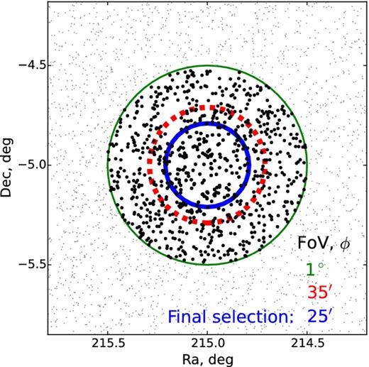
The plot shows stars in one of the Gaia-ESO Milky Way field, GES_MW_142000-050000. Small dots are surrounding stars, while the large dots are stars involved in the calculation of the selection function (see Section 6 for details). Green thin line – a 1-deg (diameter) field-of-view; red dashed line – a 35 arcmin (diameter) field-of-view; blue solid line – final target selection with a 25 arcmin (diameter) field-of-view (i.e. that at FLAMES on VLT).
One of the three main FLAMES components is a Fibre Positioner (OzPoz) which hosts two plates. While one plate is observing, the other plate is configuring fibres so that they are positioned for the subsequent observation. This limits the overhead between one observation and the next to less than 15 min, including the telescope preset and the acquisition of the next field. The fibre facility is equipped with two sets of 132 and 8 fibres to feed two different spectrographs GIRAFFE and UVES, respectively.
The medium resolution spectrograph GIRAFFE with the two setups – HR10 (λ = 533.9–561.9 nm, R ∼ 19 800) and HR21 (λ = 848.4–900.1 nm, R ∼ 16 200) was used to observe the Milky Way field stars. To observe Milky Way field stars in high-resolution mode, the survey used the UVES with a setup centred at 580 nm (λ = 480–680 nm, R ∼ 47 000; Dekker et al. 2000).
3 TARGET SELECTION METHODS
The Gaia-ESO Survey is designed to select and observe three classes of targets in the Milky Way – field stars, candidate members of open clusters and calibration standards (Gilmore et al. 2012; Randich et al. 2013). In this paper, we present the Gaia-ESO Survey selection function only for the Milky Way field stars observed with the GIRAFFE and UVES spectrographs at VLT, not including the bulge. All targets were selected according to their colours and magnitudes, using photometry from the VISTA Hemisphere Survey (VHS; McMahon et al. 2013) and the Two Micron All-Sky Survey (2MASS; Skrutskie et al. 2006). Selected potential target lists were generated at the Cambridge Astronomy Survey Unit (CASU) centre.
We discuss the initial GIRAFFE and UVES target selection and photometry used in more detail in Sections 4 and 5. In the following section, we present the basic scheme constructed to select Milky Way field targets.
3.1 Basic target selection scheme
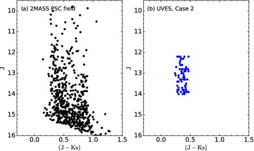
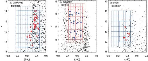
The primary goal of the selection strategy of the survey is to select Milky Way stars in order to study a robust sample of all major Galactic components (i.e. thin and thick discs, and halo). The basic target selection is built on stellar magnitudes and colours. The targets are selected to sample the main sequence, the turn-off, and the red giant branch stars centred on the red clump. To achieve this the stars are selected from two boxes, the blue and the red (see Fig. 2a). The blue box is used for the selection of the turn-off and main-sequence targets to be observed with GIRAFFE. The red box is defined to select stars on the red clump or nearby the red clump in the Colour Magnitude Diagram (CMD). For the selection of stars to be observed with UVES only one box is used (see Fig. 2b).
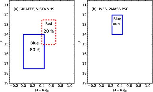
The basic colour–magnitude schemes for target selection (a) GIRAFFE and (b) UVES, respectively. Blue solid line – shows the area from which targets are assigned to the blue box, and the red dashed line – to the red box. The selection of targets is based on VISTA VHS photometry and 2MASS photometry as indicated. On the x-axis we show the dereddened (J−Ks)0 colour, whereas on the y-axis we show the observed J magnitude (for more details see Section 3.2.3).
3.2 Actual target selection schemes
We divide the selection of stars in the Milky Way fields into two cases, which are described in the following sections.
3.2.1 Case 1
Case 1, which depends on the stellar density, occurs when the field does not have enough targets to fill the FLAMES fibres (e.g. high latitude Milky Way fields). Figs 3(a) and (b) show the actual target selection colour–magnitude schemes for Case 1 for GIRAFFE and UVES, respectively. The target selection algorithm is then extended at the right-edge of the blue boxes (see black dash–dotted box in Figs 3a and b, and equations 4 and 5), allowing for the selection of second priority targets. We select second priority targets in the extra box only when all targets in the blue box have already been selected. In addition, in this case the second priority objects were selected with a colour-dependent J magnitude cut to avoid too faint targets, which would lead to low signal-to-noise ratios (S/N) in the optical spectra. This allows us to also extend the box to slightly fainter magnitudes (see Figs 3a and b).
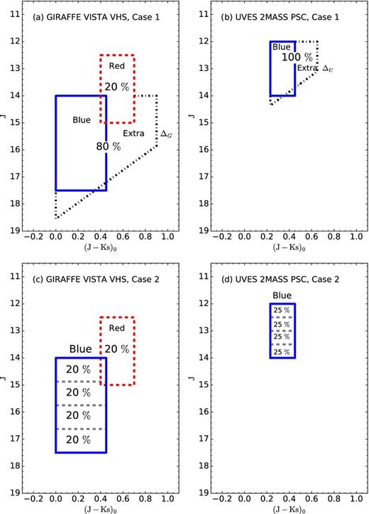
The actual target selection colour–magnitude schemes: (a) and (c) for GIRAFFE, and (b) and (d) for UVES. Target selection based on Case 1 are shown in (a) and (b), and on Case 2 in (c) and (d), respectively. Blue solid line shows the area of targets assigned to the blue box; red dashed line – to the red box; and black dash–dotted line shows the area of second priority targets assigned to the extra box. The right-edge limit (a) ΔG and (b) ΔU in Case 1 of the extra box varies from field to field. The blue box in (c) and (d) for Case 2 is divided into four equal-sized magnitude bins (in order to have the same number of targets per magnitude bin). On the x-axis we show the dereddened (J−Ks)0 colour, whereas on the y-axis we show the observed J magnitude (for more details see Section 3.2.3).
Here ΔG and ΔU are the right-edge extensions of the extra box for GIRAFFE and UVES, respectively (see black dash–dotted line in Figs 3a and b). Furthermore, these extensions vary slightly from field to field. The values for each field are shown in Fig. 4 and listed in Table 1.
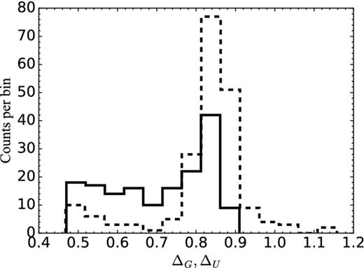
The frequency distribution of extensions ΔG and ΔU (see Section 3.2.1). The dashed line show the right-edge extensions ΔG for GIRAFFE and solid line show the right-edge extensions ΔU for UVES in Case 1 Milky Way fields.
Main parameters and weights of the targeted and allocated Milky Way fields. The full table is available online.
| GES_FLD (1) | RA [h:m:s] (2) | Dec [°:′:′] (3) | E(B−V) (4) | ΔG (5) | ΔU (6) | W_T,F_b_G (7) | ... a | Blue(per cent) (33) |
|---|---|---|---|---|---|---|---|---|
| GES_MW_000000-595959 | 00:00:00.000 | −59:59:59.99 | 0.012 | 0.834 | 0.834 | 0.225 | ... | 0.800 |
| GES_MW_000024-550000 | 00:00:24.000 | −55:00:00.00 | 0.013 | 1.033 | 0.613 | 0.272 | ... | 0.800 |
| GES_MW_000400-010000 | 00:04:00.000 | −01:00:00.00 | 0.034 | 0.923 | 0.763 | 0.275 | ... | 0.800 |
| GES_MW_000400-370000 | 00:04:00.000 | −37:00:00.00 | 0.010 | 0.855 | 0.785 | 0.237 | ... | 0.800 |
| GES_MW_000400-470000 | 00:04:00.000 | −47:00:00.00 | 0.009 | 0.905 | 0.636 | 0.209 | ... | 0.800 |
| ... | ... | ... | ... | ... | ... | ... | ... | ... |
Note.aFor column names and description see Table A1.
3.2.2 Case 2
Case 2 is encountered when the density of stars exceeds the number of fibres available. This algorithm is applied to the Milky Way fields near to the Galactic plane. In Case 2, the target selection algorithm selects targets in such way as to have the same number of targets per magnitude bin (i.e. not to have a bias towards very faint stars). Therefore, the blue box is divided into four equal-sized magnitude bins, with J1,2,3,4 = (Jmax − Jmin)/4, where J1 is the bright limit, and J4 is the faint limit of the J magnitude (see Figs 3c and d). In this case, we have no priorities for what to select within each given sub-box, so the choice is approximately random. We select approximately the same number of stars in each sub-box. The target selection magnitudes and colours for Case 2 follow the same selection limits as presented for the main target selection (see equations 1–3).
3.2.3 Extinction and colour range
The Milky Way fields located near the Galactic plane often suffer from considerable interstellar extinction. The Gaia-ESO Survey target selection algorithm takes the line-of-sight interstellar extinction, AV, into account using the Schlegel dust map (Schlegel, Finkbeiner & Davis 1998). Schlegel et al. indicate an accuracy of 16 per cent on their map. Although in the near-infrared the impact of extinction, while expected to be low, cannot be neglected, i.e. E(J − KS) = (c.J−c.Ks)*AV = 0.17*AV, which leads to approximate E(J − KS) = 0.10 for E(B − V) = 0.20 (Rieke & Lebofsky 1985). Here c.J and c.KS designate the extinction coefficients in the J and KS bands (c.J = AJ/AV and c.KS = A|$_{K_s}$|/AV) (Nishiyama et al. 2009).
The line-of-sight interstellar extinction for the GIRAFFE and UVES fields was treated differently. The line-of-sight interstellar extinction was taken into account by shifting the colour-boxes of GIRAFFE targets by 0.5*E(B − V). Whereas for UVES targets instead the box was extended to the right (i.e. the blue edge stays fixed) by 0.5*E(B − V). No shift was applied to the GIRAFFE and UVES boxes in the vertical, magnitude, direction. Here, E(J − KS)/E(B − V) = 0.5 (Rieke & Lebofsky 1985) and we take E(B − V) as the median reddening in the field measured from Schlegel et al. (1998) maps.
The median E(B − V) values vary per field and are listed in Table 1. The mean of the line-of-sight reddening for the Gaia-ESO Survey observed in Case 1 Milky Way field stars never reaches values greater than E(B − V) = 0.10, and for fields near the Galactic plane not greater than E(B − V) = 1.23. The mean line-of-sight reddening value for Case 1 fields is < E(B − V) > = 0.03 ± 0.02. For Case 2, Milky Way fields located near the Galactic plane the mean line-of-sight reddening value is < E(B − V) > = 0.10 ± 0.12.
3.2.4 Naming conventions
The Gaia-ESO Survey Milky Way field names were created at CASU from the right ascension ‘hms' and declination ‘dms' (J2000) of the field centre. For example, the Gaia-ESO Survey Milky Way field centred at RA = 14h20m00s and Dec = −05°00′00′ was assigned the name GES_MW_142000-050000. The names of the selected targets (objects) also encode which selection criteria were used to select them. ‘|$\_b\_$|' means the blue box, ‘|$\_r\_$|' the red box, and ‘|$\_e\_$|' is for the extra box (identifies the objects which were added to fill the fibres). Some of the targets were selected by both blue and red boxes, and they have ‘|$\_br\_$|' in their name.
In the fits headers of the data files the Milky Way fields can be identified with the keyword ‘|${\it {GES}}\_{\it {TYPE}}$|'. For the Milky Way fields it is set to ‘|${\it {GE}}\_{\it {MW}}$|'.
3.2.5 The Milky Way field pattern
The distribution of observed Milky Way fields in the Gaia-ESO Survey is designed to be well spread. However, the observation range in the Galaxy is restricted to +10° ≥ Dec ≥ −60° to minimize the airmass. Fig. 5 shows the distribution of so far observed fields on the sky. Table 2 lists the number of observed Milky Way fields in the Gaia-ESO Survey up to 2015 June and the number of Milky Way fields in iDR4. For these fields targets were selected as outlined in the preceding sections.
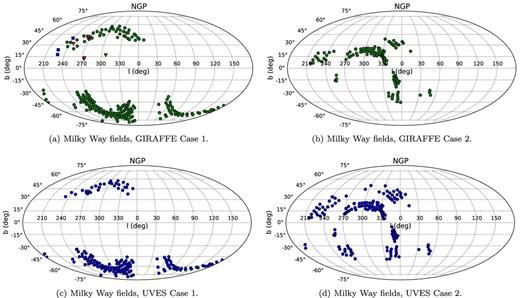
The distribution, shown in Mollweide projection with the Galactic centre in the middle, of the observed Milky Way fields across the sky. (a) and (b) show fields selected based on Cases 1 and 2, respectively, and observed with GIRAFFE. (c) and (d) show fields selected based on Cases 1 and 2, respectively, and observed with UVES. Green circles – fields with the selection based on VISTA VHS photometry; blue circles – fields with the selection based on 2MASS photometry. Additional fields: blue squares – fields with the selection based on SDSS photometry and 2MASS photometry; and red triangles – fields with the selection based on SkyMapper photometry, VISTA VHS photometry and 2MASS photometry (for more information see Appendix B).
The number of Milky Way fields observed in the Gaia-ESO Survey up to 2015 June and in iDR4.
| Instrument | VHS Case 1 | VHS Case 2 | 2MASS Case 1 | 2MASS Case 2 | SDSSa | SkyMappera | Total |
|---|---|---|---|---|---|---|---|
| GIRAFFE | 202 | 118 | – | – | 3 | 7 | 330 |
| UVES | – | – | 164 | 166 | – | – | 330 |
| iDR4 GIRAFFE | 158 | 90 | – | – | 2 | 7 | 257 |
| iDR4 UVES | – | – | 128 | 135 | – | – | 263 |
Note.aSDSS photometry and SkyMapper photometry were used to select additional targets (See Appendix B).
A small subset of additional Milky Way field targets were selected using SDSS and SkyMapper photometry in order to study metal-poor stars and K giants. Some details on the selection of these targets are given in Appendix B.
4 INITIAL GIRAFFE TARGET SELECTION
4.1 Photometric catalogue
The survey input and target selection catalogue is the VHS for the Milky Way fields observed with GIRAFFE (McMahon et al. 2013). The target selection is based on the panoramic wide field infrared VHS. The VHS survey data consists of three survey components: VHS Galactic Plane Survey (VHS-GPS); VHS-ATLAS and VHS-Dark Energy Survey (VHS-DES). In particular, catalogue versions from 2011 to 2014 were used to select Milky Way field targets. VISTA VHS has a sufficient sky coverage to meet the full science goals of the Gaia-ESO Survey. This catalogue is ∼30 times deeper than the 2MASS in at least two wavebands (J and KS) (McMahon et al. 2013) (see more about VISTA VHS2). The adopted data quality flags to select Milky Way field targets from the VHS catalogue are listed in Table 3.
Adopted data quality flags for VHS photometry (GIRAFFE) and 2MASS photometry (UVES), and SDSSa photometry.
| Catalogue | Requirement | Notes |
|---|---|---|
| VHS mergedClass | mergedClass = −1 | Classified as a star. |
| VHS jAverageConf, ksAverageConf | jAverageConf > 95, ksAverageConf > 95 | Average confidence in J, KS mag. |
| VHS jErrBits, ksErrBits | jErrBits = 0, ksErrBits = 0 | Warning/error bitwise flags in J, KS mag. |
| VHS Not on the bad CCD | jx < 8000 or jy < 12300 | Flags used in internal release. |
| 2MASS ph_qual | |$ph\_qual=AAA$| | Photometric quality flag. |
| SDSS mode | mode = 1 | Flag indicates primary sources. |
| SDSS gc | type = 6 | Phototype in g band, 6 = Star |
Note.aSDSS photometry was used to select additional targets (See Appendix B1).
The target selection magnitude and colour limits for GIRAFFE are presented in Sections 3.1 and 3.2.
4.2 Target selection Cases 1 and 2
An example of the target selection for Case 1 is shown in Fig. 6. Here, the selected blue circles are targeted turn-off and main-sequence stars to be observed with GIRAFFE, and the red squares are red clump stars. An example of the target selection for Case 2 is shown in Fig. 7. For Case 2, the target selection algorithm selected roughly the same number of blue box targets per J magnitude bin.
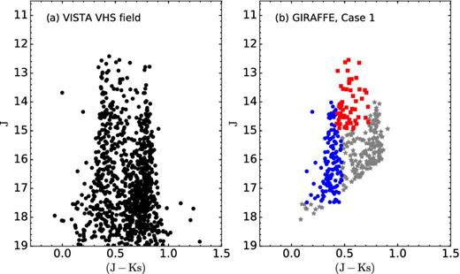
Colour–magnitude diagrams with VISTA VHS photometry. (a) CMD of the field GES_MW_142000-050000 centred at Galactic longitude l = 339| $_{.}^{\circ}$|9 and latitude b = 51| $_{.}^{\circ}$|4, and FoV = 35 arcmin in diameter. (b) GIRAFFE target selection based on Case 1 selection scheme (see Section 3.2.1). Blue circles – selection of targets in blue box; red squares – selection of targets in red box; and grey stars – second priority targets, respectively.
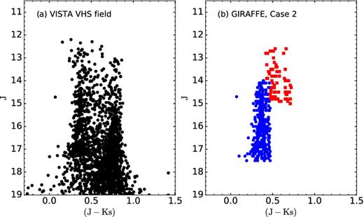
Colour–magnitude diagrams with VISTA VHS photometry. (a) CMD of the field GES_MW_201959-470000 centred at Galactic longitude l = 352| $_{.}^{\circ}$|7 and latitude b = −34| $_{.}^{\circ}$|2, and FoV = 35 arcmin in diameter. (b) GIRAFFE target selection based on Case 2 selection scheme (see Section 3.2.2). Blue circles – selection of targets in blue box; red squares – selection of targets in red box, respectively.
As mentioned before, for most of the Milky Way fields the initial target selection algorithm tried to assign 80 per cent of the targets to the blue box and 20 per cent to the red box, respectively. The selection for some of the fields near the Galactic bulge were the only fields where the selection of a blue versus red box fraction was changed, i.e. from 80/20 per cent to 20/80 per cent, to predominantly observe star the Galactic bulge direction, i.e. the red clump stars. Those Milky Way fields are indicated in the last column of Table 1.
5 INITIAL UVES TARGET SELECTION
The Gaia-ESO Survey uses UVES with the U580 setup (470–684 nm) to observe Milky Way field stars. Up to seven separate objects (plus one sky fibre) can be allocated and observed simultaneously in the U580 mode. The methodology adopted in the Gaia-ESO Survey is such that the Milky Way field observations with UVES are made in parallel with the GIRAFFE field star observations. This means that the exposure times are planned according to the observations being executed with the GIRAFFE fibres. The UVES targets are chosen according to their near-infrared colours to be FG-dwarfs/turn-off stars with magnitudes down to J2MASS = 14 mag.
The target selection box for UVES was defined using the 2MASS Point Source Catalog (2MASS PSC) photometry (Skrutskie et al. 2006). VISTA VHS photometry suffers saturation in the relevant magnitude range, while 2MASS delivers better photometry.
As for the case of GIRAFFE, the Schlegel et al. (1998) dust map, AV, was used to determine the median extinction in the field. The 2MASS catalogue flag used to select Milky Way field targets is given in Table 3. The target selection algorithm for UVES is configured using the same methodology as for GIRAFFE and is presented in Sections 3.1 and 3.2. There is only one difference in the target selection limits for UVES targets. The UVES target selection for six Milky Way fields based on Case 1 and for 20 fields for Case 2 have the brightest cut on J2MASS of 11 instead of 12 mag and these are listed in Table 4. The target selection maximum magnitude range for UVES in J2MASS is 2.0 mag within the narrow range of (J − KS). Figs 8 and 9 show the UVES target selection for two Milky Way fields for Cases 1 and 2, respectively.
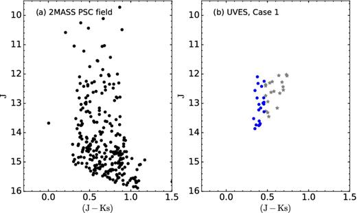
Colour–magnitude diagrams with 2MASS PSC photometry. (a) CMD of the field GES_MW_142000-050000 centred at Galactic longitude l = 339| $_{.}^{\circ}$|9 and latitude b = 51| $_{.}^{\circ}$|4, and FoV = 35 arcmin in diameter. (b) UVES target selection based on Case 1. Blue circles – selection of targets in the blue box, and grey stars – extra targets, respectively.
Colour–magnitude diagrams with 2MASS PSC photometry. (a) CMD of the field GES_MW_201959-470000 centred at Galactic longitude l = 352| $_{.}^{\circ}$|7 and latitude b = −34| $_{.}^{\circ}$|2, and FoV = 35 arcmin in diameter. (b) UVES target selection based on Case 2 showing the selected targets in the blue.
UVES Milky Way fields with J = 11 mag selection limit.
| Case 1 |
|---|
| GES_MW_025559-003000 |
| GES_MW_031800-003000 |
| GES_MW_033800-273000 |
| GES_MW_033959-000000 |
| GES_MW_092800-003000 |
| GES_MW_112200-100000 |
| Case 2 |
| GES_MW_041959-001959 |
| GES_MW_050000-520000 |
| GES_MW_070359-423000 |
| GES_MW_072048-003000 |
| GES_MW_074500-423000 |
| GES_MW_075600-090000 |
| GES_MW_075959-003000 |
| GES_MW_100000-410000 |
| GES_MW_105959-410000 |
| GES_MW_120000-410000 |
| GES_MW_124224-130559 |
| GES_MW_130047-410000 |
| GES_MW_140000-100000 |
| GES_MW_140000-410000 |
| GES_MW_145800-410000 |
| GES_MW_150159-100000 |
| GES_MW_155400-410000 |
| GES_MW_155959-003000 |
| GES_MW_170024-051200 |
| GES_MW_173359-430000 |
6 FINAL TARGET SELECTION: ALLOCATING THE FIBRES
The selected potential target lists were generated using the methodology presented in Sections 3.1 and 3.2. Thereafter, the observing team generated the final target allocation catalogue that was used for the actual observations at the VLT.
The target list has a larger FoV (35 arcmin) in diameter than the FoV for FLAMES and hence has a larger number of targets per field than can be allocated on FLAMES (see Fig. 1 and red filled circles versus blue squares in Fig. 10). This large size of the potential target list is motivated by the fact that for each observing block a guide star must also be allocated and that it is of interest to allocate as many fibres as possible. To allow for some flexibility of the centre of the final field the list of potential targets hence covers a larger area on the sky. The centres of the allocated target lists are close to the original field centres.
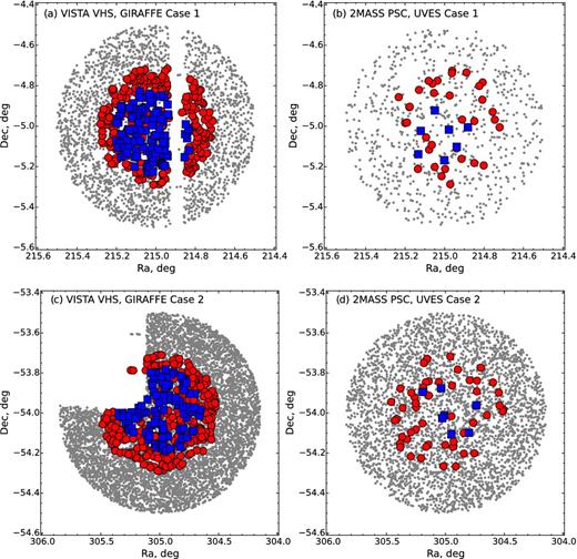
Spatial target distribution on the sky. (a) and (b) Milky Way field GES_MW_142000-050000 centred at Galactic l = 339| $_{.}^{\circ}$|9 and b = 51| $_{.}^{\circ}$|39, and selected based on Case 1 and VISTA VHS, 2MASS photometry; and (c), (d) field GES_MW_201959-540000 centred at Galactic l = 344| $_{.}^{\circ}$|3 and b = −34| $_{.}^{\circ}$|5, and selected based on Case 2, respectively. Grey dots – targets distributed in a 1 deg2 FoV in diameter; red filled circles – targets within 35 arcmin FoV in diameter; blue filled squares – allocated FLAMES targets, with 25 arcmin FoV in diameter.
The observing team uses the Fibre Positioner Observation Support Software (fposs; see the user manual3 for more details), which is the fibre configuration program for the preparation of FLAMES observations. fposs takes as input a file containing a list of target objects and generates a configuration in which as many fibres as possible are allocated to targets, allowing for the various instrumental constraints and any specified target priorities. It produces a file containing a list of allocations of fibres to targets, the so-called target setup file.
The final Gaia-ESO Survey target selection function depends on the allocated and observed targets. An illustration of two fields from Case 1 and Case 2 is shown in Fig. 10. Here, targets are shown spatially distributed on the sky within the three different field-of-view introduced in Fig. 1 and discussed earlier in this section. Grey dots show targets distributed in a 1 deg2 FoV in diameter; red filled circles show targets within 35 arcmin FoV in diameter (the one used to make the allocations); and blue filled squares show allocated FLAMES targets, with 25 arcmin FoV in diameter for two different Milky Way fields centred at Galactic longitude l = 339| $_{.}^{\circ}$|9, latitude b = 51| $_{.}^{\circ}$|39 and l = 344| $_{.}^{\circ}$|3, b = −34| $_{.}^{\circ}$|5, respectively.
There are several interesting points to extract from this illustration. First, it can be seen by visual inspection that Figs 10(a) and (c) show the incompleteness of the VISTA VHS catalogue at the time when the catalogue was used for GIRAFFE target selection. Figs 10(a) and (b) show Case 1 for GIRAFFE and UVES, respectively. In this example, a total of 111 targets (including 33 second priority targets) were allocated on FLAMES/GIRAFFE for the Milky Way field centred at Galactic longitude l = 339| $_{.}^{\circ}$|9 and latitude b = 51| $_{.}^{\circ}$|39 (Fig. 10a). The total number of allocated targets on FLAMES/UVES for the same field is seven (including three as second priority targets) (Fig 10b). The rest of the fibres were sky fibres. Figs 10(c) and (d) show an example of Case 2, for the field GES_MW_201959-540000 centred at Galactic l = 344| $_{.}^{\circ}$|3 and b = −34| $_{.}^{\circ}$|5. A total of 104 fibres were allocated (with ∼ 80 per cent from the blue box and ∼20 per cent from the red box) for GIRAFFE and seven for UVES.
7 WEIGHTS
7.1 Targeted and allocated weights
The selection function presented here consists of two steps. The first step is where potential targets are selected for GIRAFFE and UVES. The second step, final target allocation, is generating the actual list for observation.
Here, we present the weights per field calculated after the target selection and allocation. These weights can be used to better understand the Gaia-ESO Survey results and correct them for selection bias.
Since the target selection function is complex, we calculated weights for all the CMD colour boxes separately (i.e. blue, red and extra) (Figs 11 and 12). For Case 2, we calculated the blue box weights per J1–4 magnitude bins in each field within the given FoV (Figs 13 and 14). Hereafter, J1–4 = (Jmax − Jmin)/4, where J1 is the bright limit, and J4 is the faint limit of the J magnitude. All calculated CMD weights per field are listed in Table 1.
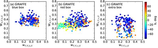
Weights of each field for targeted stars versus stars in the field within a 1 deg FoV in diameter compared with weights for allocated versus targeted stars in (a) blue, (b) red and (c) extra boxes for GIRAFFE. The colour coding indicates Galactic latitude in degrees.
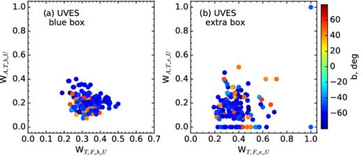
Weights of each field for targeted stars versus stars in the field within a 1 deg FoV in diameter compared with weights for allocated versus targeted stars in (a) blue and (b) extra boxes for UVES. The colour coding indicates Galactic latitude in degrees.
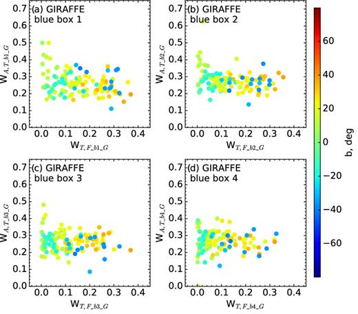
Weights of each field for targeted stars versus stars in the field within a 1 deg FoV in diameter compared with weights for allocated versus targeted stars in blue box for GIRAFFE. (a)–(d) show weights in J1–4 magnitude bins in fields within given FoV. The colour coding indicates Galactic latitude in degrees.
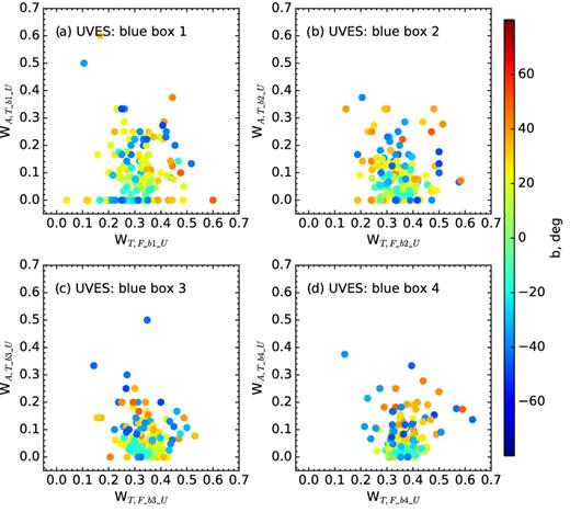
Weights of each field for targeted stars versus stars in the field within a 1 deg FoV in diameter compared with weights for allocated versus targeted stars in blue box for UVES. (a)–(d) show weights in J1–4 magnitude bins in fields within given FoV. The colour coding indicates Galactic latitude in degrees.
To illustrate the importance of accounting for the selection biases for individual Milky Way fields we show an example of the weight of the red box (WT, F) distribution in the Milky Way fields (see Fig. 15). Case 1 Milky Way fields have higher WT, F values than the Case 2 fields, but at the same time, the WT, F values are different for each individual field within the two cases.
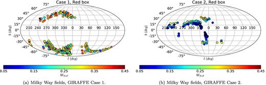
The distribution, shown in Mollweide projection with the Galactic centre in the middle, of the observed Milky Way fields across the sky. (a) and (b) show fields selected within the red box based on Cases 1 and 2, respectively, and observed with GIRAFFE. The colour coding indicates the weight WT,F (equation 8).
In order to use Milky Way field stars for a specific science question, we must understand how the spectroscopic sample is drawn from the underlying population. As can be seen from Fig. 15, the completeness of the Gaia-ESO Survey varies substantially between fields. For each field, we must therefore assess how representative the spectroscopic sample is of the underlying population. To correct for these types of biases the presented weights, WT, F; WA, T, should be used.
7.2 Using iDR4: stellar weights for the colour–magnitude diagram
The selection function presented in this paper corrects for the discrepancy between the number of stars allocated to be observed and the number of stars originally available from the photometry for each field. This enables any comparison of fields to account for the varying population densities associated with different lines of sight.
In order to ensure a completely fair comparison of the data, however, a second correction is needed. Within each field, the density of stars available for observation varies considerably with respect to both colour and magnitude. Furthermore, not all observed stars end up with reasonable parameters; a significant proportion of observations fail to produce high enough quality spectra to enable robust stellar parameter determination. Naturally, the fainter targets are more likely to fail, due to the lower S/N of the spectra obtained. This is shown clearly in Fig. 16, where all stars observed in iDR4 that failed to result in stellar parameters are plotted on the colour–magnitude diagram. There are 3849 stars in the blue box without parameters (e.g. Teff, log(g), [Fe/H]), and 856 in the red box.
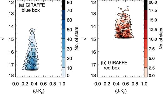
Distribution of the Milky Way field stars observed in iDR4, GIRAFFE that did not receive recommended stellar parameters in the same data release. These are split into the blue (a) and red (b) boxes.
To correct for these biases, each star that has values for the recommended stellar parameters in iDR4 needs a second weighting. This will ensure that results from the data release can be properly interpreted in terms of the actual populations of the Milky Way.
7.2.1 The CMD grids
To calculate the weights for iDR4 stars, we divide the colour–magnitude diagram into a grid of bins. The bin size is sufficiently small to accurately reflect the local sampling around each observed star. An example field is shown in Figs 17(a) and (b), and it can be seen that the grid is larger than the original selection box. We are using the latest VISTA VHS photometry to calculate these weights, however many of the fields were observed some time ago, and the selection was completed with an older version of the VISTA VHS catalogues. The magnitudes in the updated catalogues differ from the older catalogues by a very small amount, but these differences are enough to mean that some stars which previously fell inside the selection box now lie slightly outside. The larger grid allows us to include weights for those stars as well. The red box is divided into bins of size 0.05 in (J − KS), and 0.5 in J. The grid for the blue box was designed to overlap with the four magnitude boxes that were defined in Section 3.2.2 for Case 2 fields. Therefore the bins are 0.4375 long in J (half the size of the magnitude boxes J1–4), and again 0.05 wide in (J − KS).
The colour–magnitude diagrams of an example of Milky Way field (GES_MW_023959-560000) for both the blue (a) and red (b) boxes for GIRAFFE and (c) blue box for UVES. In (a) and (b) the background VISTA VHS and (c) 2MASS photometry (black points) and successfully observed targets (red and blue points) are shown. The red and blue solid lines outline the boxes used to select the targets, and the dashed lines show the grid of bins for weighting.
A similar setup is used for the UVES blue box (see Fig. 17c) as in the GIRAFFE blue box, with different sized magnitude bins again to match the boxes in Case 2 fields; the bins are 0.5 long in J, and remain 0.05 wide in (J − KS). In order to cope with those fields which had a bright limit of J2MASS = 11 rather than J2MASS = 12, the grid has been extended, as shown in Fig. 17(c).
7.2.2 Weights of successfully observed targets
CMD weights of successfully observed stars with GIRAFFE in iDR4. The full table is available online.
| CNAME | GES_FLD | RA(deg) | Dec(deg) | W_O,F_G | W_Total_G | Box |
|---|---|---|---|---|---|---|
| 00000301-5455591 | GES_MW_000024-550000 | 0.0125 | −54.9331 | 0.133 3333 | 0.017 3717 | Blue |
| 00000377-5506384 | GES_MW_000024-550000 | 0.0157 | −55.1107 | 0.200 0000 | 0.026 0576 | Blue |
| 00000395-5458308 | GES_MW_000024-550000 | 0.0165 | −54.9752 | 1.000 0000 | 0.130 2880 | Blue |
| 00000533-5459505 | GES_MW_000024-550000 | 0.0222 | −54.9974 | 0.250 0000 | 0.032 5720 | Blue |
| 00000648-5451013 | GES_MW_000024-550000 | 0.0270 | −54.8504 | 0.150 0000 | 0.019 5432 | Blue |
| ... | ... | ... | ... | ... | ... | ... |
CMD weights of successfully observed stars with UVES in iDR4. The full table is available online.
| CNAME | GES_FLD | RA(deg) | Dec(deg) | W_O,F_U | W_Total_U |
|---|---|---|---|---|---|
| 00000009-5455467 | GES_MW_000024-550000 | 0.0003 | −54.9296 | 0.200 00 | 0.016 92 |
| 00001749-5449565 | GES_MW_000024-550000 | 0.0728 | −54.8323 | 0.166 67 | 0.014 10 |
| 00012216-5458205 | GES_MW_000024-550000 | 0.3423 | −54.9723 | 0.142 86 | 0.012 08 |
| 00035430-0058050 | GES_MW_000400-010000 | 0.9762 | −0.9680 | 0.250 00 | 0.009 12 |
| 00035518-0047502 | GES_MW_000400-010000 | 0.9799 | −0.7972 | 0.333 33 | 0.012 17 |
| ... | ... | ... | ... | ... | ... |
8 A FIRST LOOK AT iDR4 SUCCESSFULLY ANALYSED DATA
As we mentioned before the selection function consists of several steps. In addition to selection and allocation of targets, we also need to know the completeness of the successfully analysed Gaia-ESO Survey Milky Way field sample, especially to understand the bias introduced by the S/N variation in the observed FLAMES spectra. Therefore we looked at the Gaia-ESO Survey iDR4 data. The internal DR4 is a full release. All observations from the beginning of the survey until 2014 July are included.
Not surprisingly, the S/N varies with J magnitude. We made a potential quality cut on S/N ratio of the spectra. Inspecting the spectroscopic results (e.g. Teff, [Fe/H]) we chose to cut the spectroscopic sample at a median S/N > 20. This cut might be different if one wants to consider other spectroscopic results e.g. alpha abundance. Fig. 18 shows the relation between the potential photometric sample (black contours), the spectroscopic sample (green contours), and after the quality cut on S/N (yellow contours) for the Milky Way field GIRAFFE sample. In our case, while the sampling in colour is close to unbiased, the sampling in J is strongly biased against faint targets because of the signal-to-noise cut (S/N > 20). Similar trends are seen in the SEGUE G-dwarf sample analysed by Bovy et al. (2012). Introducing this quality cut we lose about one magnitude in depth for targets within the blue box, while the sampling in the red box is not that affected (see Fig. 18).
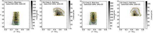
Distribution of the photometric sample of the Gaia-ESO Survey Milky Way fields in blue (a, c) and red (b, d) boxes (linear density grey-scale, black contours). The observed spectroscopic sample of the Gaia-ESO Survey iDR4 is shown as green contours; yellow contours show the spectroscopic sample with determined effective temperature and the signal-to-noise ratio cut of S/N > 20. The black, green and yellow contours contain 68, 95 and 99 per cent of the distribution of Case 1 and Case 2 Milky Way field stars. On the x-axis we show the dereddened (J−Ks)0 colour, whereas on the y-axis we show the observed J magnitude.
Stars observed with GIRAFFE that are in the region of the CMD where blue and red boxes overlap will have two WTotal weights and will be indicated in Table 5 as blue/red (calculated as blue box star) or red/blue (calculated as red box star) targets. Our recommendation is to use the blue box weight for those stars (607 stars in iDR4) when combining blue and red box data.
We can therefore, when trying to accurately sample the Milky Way disc, characterize the importance of an observed star in iDR4 by giving it a weight. In order to make a correction for each successfully observed star in our sample, we give the total weight WTotal as 1/WTotal. Here we effectively tell how frequent a successfully observed stars is with a given J and (J − Ks) within a given Milky Way field in a given FoV. In this example we chose to remove stars where 1/WTotal > 100 000, because in this case the weight is too large to be meaningful, and the star is not representative of the sample. Essentially, this cut removes 1.2 per cent of blue box targets and 0.2 per cent of red box targets.
In Fig. 19, we show an application of the weights presented in this paper. We see that the metallicity distribution of stars observed in the Gaia-ESO Survey iDR4 with GIRAFFE in the blue and red boxes (blue and red line) are different from the weighted distributions (black dashed line) when all Milky Way fields are analysed together. We find that for the red box the observed distribution is the same as the underlying distribution, but this is not the case for the blue box, as seen by comparing their respective cumulative distributions, corrected versus uncorrected (see Figs 19c and d). The total weight, WTotal, normalizes between the different lines of sight; while each observed Milky Way field has almost the same number of spectra, but not the same number of successfully analysed stars and different number of photometric objects varying per line of sight due to the nature of the Galaxy. This is a simple example to highlight the necessity of including such information in studies of the stellar populations in the Milky Way. There are other ways how one can apply presented weights (i.e. taking into account the [Fe/H] errors, looking at different lines of site or combining blue and red box targets together).
![The metallicity distribution of all Milky Way field stars observed with GIRAFFE in the Gaia-ESO Survey iDR4. (a, c) and (b, d) show metallicity distribution of stars within blue and red boxes, respectively. The blue and red lines show the observed metallicity; the black dashed lines show weighted metallicity distributions. Only stars with [Fe/H] < 0.50 are included.](https://oup.silverchair-cdn.com/oup/backfile/Content_public/Journal/mnras/460/1/10.1093_mnras_stw1011/2/m_stw1011fig19.jpeg?Expires=1749929833&Signature=KauW-3QXD~H0jqeXSXCadsl88KEIvB06oMdfW54d7fPlZ9o7fH30RQiUC8Ye6qoa1WgObDQ9JeTwvw8gF~Sc~ch7aAuRbBr4vmpEdCyKbCdgiTh5ldsl9RCtm90xQURXipMmzoXLtaA-u4HQ06iR8ihf4xUfVLdQILPEZWuhIQLVtvywRwnoSLjx9y6xIY05zOyhzdz165vLB34CORIWTvtULiYjvCOk1EhivTGTF5pv2TH4yK61RPtIRiMsnSWCLNLyGXiOu4VV7sXnGs4LzQvE7INYwSXGGP4AseuvJa1RmCZ8JocIu0LVfwN8cEuEn-nMCY6h~J31u~3z6EOTEg__&Key-Pair-Id=APKAIE5G5CRDK6RD3PGA)
The metallicity distribution of all Milky Way field stars observed with GIRAFFE in the Gaia-ESO Survey iDR4. (a, c) and (b, d) show metallicity distribution of stars within blue and red boxes, respectively. The blue and red lines show the observed metallicity; the black dashed lines show weighted metallicity distributions. Only stars with [Fe/H] < 0.50 are included.
The presented field CMD weights (WA,T, WT,F) and the weights of successfully observed targets (|$W_{{\rm O}_{{\rm bin}},{\rm F}_{{\rm bin}}}$|) can be used differently than in the previous example. For example, looking at the radial and/or vertical metallicity distribution the weights can be used to limit the data to only those stars that most represent the underlying population. In this case, we do not want stars with very small WTotal to contribute to the analysis, since they do not provide enough information about the actual underlying population. A simple way of studying the Milky Way's radial metallicity gradient is to bin the data in Galactocentric radial distance R and compute the mean metallicity in each bin as a running average. However, instead of computing a straight mean, we can perform a weighted average, in which each star is weighted by WTotal. This will then bias the mean metallicity towards those stars with the highest WTotal. The results can then be compared with those for the standard mean to understand possible biases in the data.
9 CONCLUSIONS AND FUTURE PROSPECTS
We have discussed the details of the selection function for the Milky Way field stars observed in the Gaia-ESO Survey. The weights presented here are based on targets selected from the beginning of the survey up to the end of 2015 June. To characterize the major components of the Galaxy, and to understand these components in the context of the Milky Way's formation and evolution history, the survey selection function is designed to target stars as homogeneously as possible throughout the Milky Way. The target selection is based on stellar magnitudes and colours, using photometry from the VHS (McMahon et al. 2013) and 2MASS (Skrutskie et al. 2006). Also we present the basic and actual target selection schemes for the Milky Way field stars observed with FLAMES/GIRAFFE and FLAMES/UVES.
The actual target selection scheme is divided into two cases. In Case 1 the target selection algorithm, in addition to the two main selection CMD boxes (i.e. blue, red), extends the colour limits to select second priority targets (i.e. for those Milky Way fields where the density of stars is not enough to fill the FLAMES fibres). Case 2 is used to select targets near the Galactic plane. In this case, the target selection algorithm is configured to select the same number of targets per magnitude bin (i.e. not to have a bias towards very faint stars).
From the beginning of the survey on 2011 December 31 until 2015 June, a total of 330 Milky Way fields have been targeted and allocated on FLAMES. 202 Milky Way fields were selected using Case 1 and 118 using Case 2, which were then allocated on FLAMES/GIRAFFE. For UVES, 164 and 166 Milky Way fields were used in Case 1 and Case 2, respectively. In addition, a sample of Milky Way fields were selected to target rare but astrophysically important stellar populations (e.g. metal-poor stars, K giants), where Milky Way field targets were selected using the SDSS photometry (Ahn et al. 2012) and SkyMapper photometry (Keller et al. 2007), for allocation on FLAMES/GIRAFFE and FLAMES/UVES.
The Gaia-ESO Survey selection function depends not only on potentially selected targets but also on allocated targets. It is crucial to know the number of stars that were not allocated to any spectroscopic fibre, i.e. FLAMES/GIRAFFE fibres, in order to afterwards correct for any incompleteness effects on the survey. Finally, we presented the weights calculated after the target selection and allocation. These weights can be used to better understand the Gaia-ESO Survey results and correct selection biases for the proper interpretation of the data in terms of our understanding of the Milky Way as a galaxy.
We are continuing our work on weights application for the Gaia-ESO Survey Milky Way field GIRAFFE data and the results will be presented in a forthcoming paper. Here we presented weights per field for targeted and allocated Milky Way stars observed up to end of 2015 June and weights of successfully observed iDR4 stars 15 154 for GIRAFFE and 1367 for UVES and we plan to continue our work on the target selection function for Milky Way stars when the next data set is available.
ES, LH, SF, GRR and TB acknowledge support from the project grant ‘The New Milky Way' from the Knut and Alice Wallenberg Foundation. RS acknowledges support from NCN/Poland through grant 2014/15/B/ST9/03981. AJK acknowledges support by the Swedish National Space Board. We thank the anonymous referee for her/his constructive comments, which have improved the clarity of the paper. Based on data products from observations made with ESO Telescopes at the La Silla Paranal Observatory under programme ID 188.B-3002. These data products have been processed by the CASU at the Institute of Astronomy, University of Cambridge, and by the FLAMES/UVES reduction team at INAF/Osservatorio Astrofisico di Arcetri. These data have been obtained from the Gaia-ESO Survey Data Archive, prepared and hosted by the Wide Field Astronomy Unit, Institute for Astronomy, University of Edinburgh, which is funded by the UK Science and Technology Facilities Council. This work was partly supported by the European Union FP7 programme through ERC grant number 320360 and by the Leverhulme Trust through grant RPG-2012-541. We acknowledge the support from INAF and Ministero dell' Istruzione, dell' Università' e della Ricerca (MIUR) in the form of the grant ‘Premiale VLT 2012'. The results presented here benefit from discussions held during the Gaia-ESO workshops and conferences supported by the ESF (European Science Foundation) through the GREAT Research Network Programme. Based on observations obtained as part of the VHS, ESO Program, 179.A-2010 (PI: McMahon). Funding for SDSS-III has been provided by the Alfred P. Sloan Foundation, the Participating Institutions, the National Science Foundation, and the US Department of Energy Office of Science. The SDSS-III website is http://www.sdss3.org/.
REFERENCES
SUPPORTING INFORMATION
Additional Supporting Information may be found in the online version of this article:
Table 1. Main parameters and weights of the targeted and allocated Milky Way fields.
Table 5. CMD weights of successfully observed stars with GIRAFFE in iDR4.
Table 6. CMD weights of successfully observed stars with UVES in iDR4 (Supplementary Data).
Please note: Oxford University Press is not responsible for the content or functionality of any supporting materials supplied by the authors. Any queries (other than missing material) should be directed to the corresponding author for the article.
APPENDIX A: CALCULATED CMD WEIGHTS
For each Milky Way field observed from the beginning of the Gaia-ESO Survey until 2015 June, we calculated CMD weights per field WT, F and WA, T to correct for potential biases. Those Milky Way fields and associated field weights are in Table 1 and the meanings of acronyms used are in Table A1. Full version of Table 1 is available online.
The meanings of acronyms used in Table 1.
| Col_No | Acronym | Meaning |
|---|---|---|
| (1) | GES_FLD | GES Milky Way field name from CASU. |
| (2) | RA | RA [h:m:s] of GES Milky Way field centre. |
| (3) | Dec | Dec [d:m:s] of GES Milky Way field centre. |
| (4) | E(B−V) | The Galactic dust extinction median value measured from the Schlegel, Finkbeiner & Davis (1998) maps. |
| (5) | ΔG | The right-edge limit of second priority targets for GIRAFFE. |
| (6) | ΔU | The right-edge limit of second priority targets for UVES. |
| (7) | W_T,F_b_G | The weight of blue box for GIRAFFE, where targeted star counts are versus star counts in 1° FoV. |
| (8) | W_T,F_b1_G | The weight of blue box with J1 for GIRAFFE, where targeted star counts are versus star counts in 1° FoV. |
| (9) | W_T,F_b2_G | The weight of blue box with J2 for GIRAFFE, where targeted star counts are versus star counts in 1° FoV. |
| (10) | W_T,F_b3_G | The weight of blue box with J3 for GIRAFFE, where targeted star counts are versus star counts in 1° FoV. |
| (11) | W_T,F_b4_G | The weight of blue box with J4 for GIRAFFE, where targeted star counts are versus star counts in 1° FoV. |
| (12) | W_T,F_r_G | The weight of red box for GIRAFFE, where targeted star counts are versus star counts in 1° FoV. |
| (13) | W_T,F_e_G | The weight of extra box for GIRAFFE, where targeted star counts are versus star counts in 1° FoV. |
| (14) | W_A,T_b_G | The weight of blue box for GIRAFFE, where allocated star counts are versus targeted star counts. |
| (15) | W_A,T_b1_G | The weight of blue box with J1 for GIRAFFE, where allocated star counts are versus targeted star counts. |
| (16) | W_A,T_b2_G | The weight of blue box with J2 for GIRAFFE, where allocated star counts are versus targeted star counts. |
| (17) | W_A,T_b3_G | The weight of blue box with J3 for GIRAFFE, where allocated star counts are versus targeted star counts. |
| (18) | W_A,T_b4_G | The weight of blue box with J4 for GIRAFFE, where allocated star counts are versus targeted star counts. |
| (19) | W_A,T_r_G | The weight of red box for GIRAFFE, where allocated star counts are versus targeted star counts. |
| (20) | W_A,T_e_G | The weight of extra box for GIRAFFE, where allocated star counts are versus targeted star counts. |
| (21) | W_T,F_b_U | The weight of blue box for UVES, where targeted star counts are versus star counts in 1° FoV. |
| (22) | W_T,F_b1_U | The weight of blue box with J1 for UVES, where targeted star counts are versus star counts in 1° FoV. |
| (23) | W_T,F_b2_U | The weight of blue box with J2 for UVES, where targeted star counts are versus star counts in 1° FoV. |
| (24) | W_T,F_b3_U | The weight of blue box with J3 for UVES, where targeted star counts are versus star counts in 1° FoV. |
| (25) | W_T,F_b4_U | The weight of blue box with J4 for UVES, where targeted star counts are versus star counts in 1° FoV. |
| (26) | W_T,F_e_U | The weight of extra box for UVES, where targeted star counts are versus star counts in 1° FoV. |
| (27) | W_A,T_b_U | The weight of blue box for UVES, where allocated star counts are versus targeted star counts. |
| (28) | W_A,T_b1_U | The weight of blue box with J1 for UVES, where allocated star counts are versus targeted star counts. |
| (29) | W_A,T_b2_U | The weight of blue box with J2 for UVES, where allocated star counts are versus targeted star counts. |
| (30) | W_A,T_b3_U | The weight of blue box with J3 for UVES, where allocated star counts are versus targeted star counts. |
| (31) | W_A,T_b4_U | The weight of blue box with J4 for UVES, where allocated star counts are versus targeted star counts. |
| (32) | W_A,T_e_U | The weight of extra box for UVES, where allocated star counts are versus targeted star counts. |
| (33) | Blue(per cent) | The approximate fraction of targets in the blue versus the red box (per cent). |
APPENDIX B: ADDITIONAL FIELDS
A subset of fields were allocated to specially selected candidate targets belonging to rare but astrophysically important stellar populations, such as metal-poor stars or K giants. Those additional fields in Gaia-ESO survey are labelled as Milky Way fields. The target selection for those additional fields is different from the Milky Way fields presented in this paper. The additional fields were created with the target selection based on SkyMapper photometry (Keller et al. 2007), SDSS photometry (Ahn et al. 2012), VISTA VHS photometry and 2MASS photometry (see location of the fields on the sky in Fig. 5a). In the following sections we present those different selections.
B1 Milky way fields selected to study the outer Galactic disc
Three additional Milky Way fields were selected using SDSS photometry in order to study the outer disc of the Galaxy. GIRAFFE fibres were allocated to candidate K giants, which probe the far outer disc, warp and flare.
Milky Way fieldsa for which SDSS photometry was used to select the targets to be observe with GIRAFFE (see Appendix B1).
| Milky Way fields | ΔSDSS |
|---|---|
| GES_MW_082312-052959 | – |
| GES_MW_083959-003000 | 0.41 |
| GES_MW_095600-003000 | – |
| Milky Way fields | ΔSDSS |
|---|---|
| GES_MW_082312-052959 | – |
| GES_MW_083959-003000 | 0.41 |
| GES_MW_095600-003000 | – |
Note.aFor UVES targets the selection is based on 2MASS photometry.
B2 Milky Way fields with metal-poor stars in the halo
B2.1 Milky Way fields with the target selection based on SkyMapper photometry and 2MASS photometry
Seven additional Milky Way fields were selected using SkyMapper photometry in order to study the metal-poor stars in the halo.
All GIRAFFE targets were selected from the SkyMapper photometry. For the same Milky Way fields only one UVES fibre per field was devoted to observe a metal-poor star selected using SkyMapper photometry. The remaining UVES targets were selected using 2MASS photometry.
Milky Way field names for which SkyMapper photometry was used to select the targets to be observe with GIRAFFE and one target to be observed with UVES are listed in Table B2.
Milky Way fields for which SkyMapper photometry was used to select the targets to be observe with GIRAFFE and one target to be observed with UVESa (see Appendix B2.1).
| Milky Way fields |
|---|
| GES_MW_094753-102657 |
| GES_MW_100913-412801 |
| GES_MW_101428-405235 |
| GES_MW_105731-124726 |
| GES_MW_105808-154324 |
| GES_MW_110053-132816 |
| GES_MW_131359-460007 |
| Milky Way fields |
|---|
| GES_MW_094753-102657 |
| GES_MW_100913-412801 |
| GES_MW_101428-405235 |
| GES_MW_105731-124726 |
| GES_MW_105808-154324 |
| GES_MW_110053-132816 |
| GES_MW_131359-460007 |
Note.aThe remaining UVES targets are selected based on 2MASS photometry.
B2.2 Milky Way fields with the target selection based on SkyMapper photometry, 2MASS photometry and VISTA VHS photometry
Table B3 list additional Milky Way fields selected to study the metal-poor stars in the halo. One UVES target selected using SkyMapper photometry was dedicated to study the most interesting metal-poor star in the halo. The remaining UVES targets were selected using 2MASS photometry.
Milky Way fields with the target selection based on SkyMappera photometry, 2MASSb photometry and VISTA VHSc photometry (see Appendix B2.2).
| Milky Way fields |
|---|
| GES_MW_125609-451238 |
| GES_MW_133026-434759 |
| GES_MW_142145-440827 |
| GES_MW_144113-400831 |
| GES_MW_212402-431239 |
| GES_MW_212731-542154 |
| GES_MW_221259-455029 |
| GES_MW_221818-582824 |
| GES_MW_225008-554935 |
| GES_MW_225108-524744 |
| GES_MW_234854-560538 |
Notes.aOnly one SkyMapper target per field was observed by UVES.
bThe remaining UVES targets were selected based on 2MASS photometry.
cFor GIRAFFE targets the selection is based on VISTA VHS photometry.
For the GIRAFFE targets in the same Milky Way fields the selection is based on VISTA VHS photometry as described in Section 4.
