


Abstract
We present a new method for determining the local dark matter density using kinematic data for a population of tracer stars. The Jeans equation in the z-direction is integrated to yield an equation that gives the velocity dispersion as a function of the total mass density, tracer density, and the ‘tilt’ term that describes the coupling of vertical and radial motions. We then fit a dark matter mass profile to tracer density and velocity dispersion data to derive credible regions on the vertical dark matter density profile. Our method avoids numerical differentiation, leading to lower numerical noise, and is able to deal with the tilt term while remaining one dimensional. In this study we present the method and perform initial tests on idealized mock data. We also demonstrate the importance of dealing with the tilt term for tracers that sample ≳1 kpc above the disc plane. If ignored, this results in a systematic underestimation of the dark matter density.
1 INTRODUCTION
Dark matter (DM) is an elusive component of the cosmos. Its existence has long been inferred from its gravitational interactions with ordinary matter on scales ranging from dwarf galaxies and galactic rotation curves to lensing galaxies, galaxy clusters, and the Universe as a whole (for reviews see e.g. Rubin 1993; Jungman, Kamionkowski & Griest 1996; Bergström 2000; Bertone, Hooper & Silk 2005; Bertone 2010; Massey, Kitching & Richard 2010). However its exact nature remains unknown.
Understanding the distribution of DM in cosmological structures, and in particular in the Milky Way, is of great importance to test the standard Λcold dark matter (ΛCDM) cosmological model, to make predictions – and allow the interpretation – of experiments that seek to detect DM, and to probe more exotic models for DM (e.g. Read 2014). Here, we will focus our attention on the local DM density – i.e. the average density of DM over a small volume (typically of size ∼100–1000 pc) centred around the Sun. The local DM density is a vital input for so-called direct DM experiments, based on the detection of the recoil energy of nuclei struck by DM particles streaming through underground detectors, as the expected event rate is proportional to the local DM density and the DM–nucleon cross-section. In addition, the local DM density is important for indirect searches that look for neutrinos produced by the annihilation of DM particles trapped at the centre of Sun (see e.g. Klasen, Pohl & Sigl 2015, and references therein for a recent update on direct and indirect searches). The results of these searches are also used in explorations of theoretical parameter space, such as those of Supersymmetry (e.g. Allanach & Lester 2006; Buchmueller et al. 2014; Strege et al. 2014; Bertone et al. 2016; Roszkowski, Sessolo & Williams 2015).
Methods of determining the local DM density can be divided into two categories: those utilizing measurements of stars in a small volume around the Sun (e.g. Kapteyn 1922; Jeans 1922; Oort 1932; Bahcall 1984; Kuijken & Gilmore 1989b, 1991; Creze et al. 1998; Garbari et al. 2012; Bovy & Tremaine 2012; Smith, Whiteoak & Evans 2012; Zhang et al. 2013; Bienaymé et al. 2014) and those utilizing a host of dynamical tracers – particularly the rotation curve – to constrain more global mass models of the Milky Way (Dehnen & Binney 1998; Catena & Ullio 2010; Salucci et al. 2010; Weber & de Boer 2010; McMillan 2011; Nesti & Salucci 2013; Piffl et al. 2014; Iocco, Pato & Bertone 2015; Pato & Iocco 2015; Pato, Iocco & Bertone 2015). Following the notation of Read (2014) we denote the local DM density derived from local measurements by ρDM, and those extrapolated from rotation curves assuming a spherical DM halo as ρDM, ext. With the advent of large survey data, local and global methods are beginning to converge (Bovy & Rix 2013; Piffl et al. 2014).
The comparison of ρDM to ρDM, ext can provide insight into the shape of the Milky Way's DM halo, and thus into the formation of the galaxy (Read 2014). If ρDM from local measurements is smaller than that extrapolated from global measurements, ρDM, ext, then this implies a prolate halo, while the opposite would imply a squashed, oblate halo. While the former is produced by DM only N-body simulations, the introduction of baryons into the simulations produces the latter (Katz & Gunn 1991; Dubinski 1994; Debattista et al. 2008; Read et al. 2009).
If ρDM is derived from tracers distributed vertically in the plane it is possible to probe not only the local DM density but also its vertical profile, ρDM(z). This could potentially reveal deviations from a spherical halo profile, which can form in a number of ways. First, the DM halo should respond to the formation of the baryonic disc by flattening into an oblate halo (Katz & Gunn 1991; Dubinski 1994; Debattista et al. 2008; Read et al. 2009). Secondly, the accretion of subhaloes after the formation of the baryonic disc can also lead to the formation of a ‘dark disc’ (DD) that corotates with the baryonic disc (Lake 1989; Read et al. 2008, 2009; Purcell, Bullock & Kaplinghat 2009; Ling et al. 2010; Pillepich et al. 2014). Gravitationally these two features, an oblate halo and a DD, are indistinguishable and degenerate. One method to distinguish the two is to hunt for the chemically and kinematically distinct sub-halo stars that would accompany the accreted DD, but not the contracted DM halo. Recent Gaia-ESO observational data find no evidence for such stars (Ruchti et al. 2014, 2015), suggesting that the Milky Way has had a rather quiet past since its disc formed, and therefore does not host a significant accreted DD. If correct, then any gravitationally detected non-sphericity must imply a non-rotating locally oblate halo. An enhancement in ρDM over ρDM, ext is also a feature in some more exotic models, such as Partially Interacting Dark Matter (PIDM) (Fan et al. 2013), and some modified theories of gravity (e.g. Read & Moore 2005; Nipoti et al. 2007).
Measurement of the local DM density dates back almost 100 years (Kapteyn 1922). The history of this measurement is one of both increasingly precise data and decreasingly strong assumptions. As such, the error bars on ρDM have not always shrunk with time, as better data often allows one to discard previous assumptions. With the advent of Gaia data from 2016 onwards we will have access to high-precision data on individual stars, and the primary uncertainty in the determination of ρDM will be systematic model uncertainties. Recent results for the local DM density include Bienaymé et al. (2014), who used RAVE data to derive a value of ρDM = 0.0143 ± 0.0011 M⊙ pc−3 = 0.542 ± 0.042 GeVcm−3, and Zhang et al. (2013) who used Sloan Digital Sky Survey (SDSS)/SEGUE data to find ρDM = 0.0065 ± 0.0023 M⊙ pc−3 = 0.25 ± 0.09 GeVcm−3. Note that these two results do not overlap within their stated uncertainties. The significance of this discrepancy is hard to interpret though, as they each use different data sets and analysis techniques, and both methodologies rely on rather different assumptions. To make progress we should endeavour to minimize the number of assumptions made, and apply the same analysis techniques to both data sets.
In this paper we make progress towards the first goal of reducing model assumptions. To achieve this we introduce a one-dimensional Jeans analysis method to probe the local DM density using the vertical motions of tracer stars. We construct a representation of the tracer density ν, and also allow for a DM density profile that is more complex than simply constant with height as previous local studies have assumed. Additionally, we deal with the so-called tilt term, which links radial and vertical motions of the tracer stars. This term is crucial to understand stellar motions at high-z, where the baryonic contribution falls off and DM becomes increasingly important. Using the vertical Jeans equation we calculate the velocity dispersion σz(z) for each mass model, and then fit to data in ν, σz, and σRz using MultiNest (Feroz & Hobson 2008; Feroz, Hobson & Bridges 2009; Feroz et al. 2013). We test this method on mock data sets, and explore the impact of tracer star sample size, the tilt term, and non-constant DM profiles. The mock data for this paper are ‘as good as it gets’ – we assume the population to have no observational biases and there to be no measurement error on individual stars – allowing us to isolate the effects of sampling error and model uncertainties. This is similar to what we will have with Gaia data, where the measurement errors on stars will be small compared to sampling error. We will explore the effect of adding realistic Gaia uncertainties to our method in a separate work.
We reiterate that this method is one dimensional, allowing us to keep assumptions to a minimum. However, we show that we are still able to deal with tilt and high-z data, which usually require a two-dimensional method. The key disadvantages of our method are that we bin data and thus lose information, and that our strictly local method cannot take advantage of the ‘long lever arm’ of a global model that would ensure, for example, that the DM density in radial slices close to the ‘local volume’ is continuous and smooth. However, the effect of these disadvantages is to overestimate the errors on ρDM, which is acceptable as we aim for a conservative and robust estimate of ρDM.
The paper is organized as follows: in Section 2 we introduce our method, covering the Jeans equation based mathematical formalism, our treatment of the rotation curve and tilt term, our descriptions of the elements of our mass and tracer density models. We then outline our statistical analysis, introducing the framework for Bayesian parameter estimation and the MultiNest nested sampling code. In Section 3 we describe the array of mock data sets we use to test out methods. In Section 4 we present and discuss the results of our analyses, before finally concluding the paper with Section 5.
2 METHOD
The broad picture of our problem is this: we have quantities derived from the motions of the tracer stars, namely ν, the tracer density, σz, the vertical velocity dispersion, and σR, z, the (R, z) velocity dispersion. Then we have elements of the mass profile, one of which is unknown – the DM density ρDM, and the other which is known within a band of uncertainty – the baryon density ρbaryon. In this section we first derive the equations to link these quantities, and then describe how each is modelled.
2.1 Deriving a general 1D jeans method
Equation (3) is numerically appealing to solve since, unlike many previous methods (e.g. Garbari, Read & Lake 2011; Garbari et al. 2012), it does not require any numerical differentiation and is therefore rather robust to noise in the data. Furthermore, equation (3) is valid for any gravity theory and can therefore be used as a constraint on alternative gravity models. In this sense, we follow the early pioneering work of Hill (1960) who attempted to also measure Kz directly without reference to the Poisson equation.
Values of Oort constants. We include the F giants even though the errors for them are substantially larger to show that, within current uncertainties, the Oort constants A and B do not depend on stellar type.
Values of Oort constants. We include the F giants even though the errors for them are substantially larger to show that, within current uncertainties, the Oort constants A and B do not depend on stellar type.
The overall flow of our method is now apparent. We model the tracer density ν(z), the mass density distribution ρ(z) = ρDM(z) + ρbaryon(z) (which gives us the Kz term), the tilt term |$\mathcal {T}(z)$|, and the axial term |$\mathcal {A}(z)$|. These elements each have a number of parameters, and so in total each model will have an N-dimensional parameter space. Specifying values for each of these parameters will then give us quantitative values for each of these elements, which can then be inserted into equation (3) to derive |$\sigma _z^2(z)$| for that parameter space point. We then compare ν(z) and |$\sigma _z^2(z)$| [and σRz(z) as part of the tilt term model] to data via a χ2 test, and then change the values of our parameters.
Note that the only assumptions that go into equation (3) are that the motions of stars obey the collisionless Boltzmann equation, and that the galaxy is in dynamic equilibrium. The assumption of dynamic equilibrium can be negated somewhat by the presence of disequilibria (‘wobbling’) in the disc caused by e.g. the Sagittarius merger (Purcell et al. 2011; Gómez et al. 2013) or in part by the presence of spiral arms (Faure, Siebert & Famaey 2014). However, the impact of these effects on the measurement of the local DM density is estimated to be approximately 10 per cent (Widrow et al. 2012; Read 2014), less than the corrections arising from the tilt and rotation curve terms.
In practice, further assumptions are necessary to model the individual components on the RHS of equation (3). However, this method can accommodate almost any model for each of these elements – the only strict requirement is that each element can be defined at the z-values corresponding to the centres of the bins used to calculate the tracer density and velocity dispersion. Hence we call this method ‘non-parametric’ – we can in principle have many more parameters for each model than there are data points. In the following subsections we describe how we model each element for this particular study. In Section 2.6 we discuss model selection using the Bayesian evidence, which could potentially allow us to compare alternate models.
As the galaxy is close to being axisymmetric in both the thin disc (Dehnen 1998; Hogg et al. 2005; Aumer & Binney 2009; Bovy, Hogg & Roweis 2009; Pasetto et al. 2012b; Aghajani & Lindegren 2013) and the thick disc (Pasetto et al. 2012a; Sharma et al. 2014), the axial term |$\mathcal {A}(z)$| is expected to be small. For this study we assume complete axisymmetry, and thus take |$\mathcal {A}(z) = 0$|. If the data show significant non-axisymmetry in the Milky Way, the axial term could be modelled in a similar way to the tilt term as described below.
Note that if the axial term were non-negligible, in the context of the Milky Way, this would imply the presence of significant spiral arms or a bar. Such features are time dependent, implying that if |$\mathcal {A}(z) \ne 0$|, we should also worry about the time dependence of the gravitational potential Φ(t) and, therefore, also the partial time derivative of the distribution function ∂f/∂t (e.g. Monari, Famaey & Siebert 2016). It is not clear if there can exist a regime in which |$\mathcal {A}(z) \ne 0$| and such time dependence can be ignored. Here, we simply note that since empirically |$\mathcal {A}(z) \ll \mathcal {T}(z) \, \forall z$| (e.g. Pasetto et al. 2012a,b), to leading order we can also safely neglect the time dependence of the distribution function, as we have already done.
2.2 Tracer density model
To apply the Jeans equations we bin data to obtain the tracer density ν and the velocity dispersions σz and σRz. Thus at a bare minimum we only have to define ν and σRz, and derive σz via equation (3), at the bin centres, i.e. at a discrete set of z values.
2.3 Baryon parametrization
2.4 Dark matter parametrization
The simplest way to parametrize the DM density profile ρDM is to assume it is constant with z, as done in previous work (e.g. Bahcall 1984; Kuijken & Gilmore 1989a,b; Creze et al. 1998; Garbari et al. 2011, 2012). This assumption works well at low z: for a spherical NFW halo with a scale radius of 20 kpc the mid-plane value is correct within 10 per cent up to a height of z ∼ 3 kpc. For some analyses we also make this assumption, and set ρDM(z) = ρDM, const..
2.5 Tilt term
The tilt term from equation (2) links radial and vertical motion. The importance of this term has been noted previously, e.g. Kuijken & Gilmore (1989a), Smith, Wyn Evans & An (2009), Büdenbender et al. (2015). Here, we demonstrate that it is possible to deal with this term while remaining within our vertical, one-dimensional framework. Given the data quality currently available for the Milky Way we are required to make a well-motivated assumption about the radial form of |$\mathcal {T}$|, but in the Gaia-era we will be able to directly measure this from the data.
![σRz for two populations of G-type dwarf stars in the solar neighbourhood from the SDSS/SEGUE survey (Büdenbender, van de Ven & Watkins 2015). The blue data points are from a younger, high-metallicity population, with $\overline{[{\rm Fe/H}]} = -0.07$ and $\overline{[\alpha {\rm /H}]} = 0.11$, while the data points in red are from an older, low-metallicity population with $\overline{[{\rm Fe/H}]} = -0.89$ and $\overline{[\alpha {\rm /H}]} = 0.34$. The blue and red lines are power laws in the form of equation (20) fitted to the blue and red data points, respectively. The older, lower metallicity stars probe further above the disc plane. Dashed lines indicate extrapolation from data.](https://oup.silverchair-cdn.com/oup/backfile/Content_public/Journal/mnras/459/4/10.1093_mnras_stw917/2/m_stw917fig1.jpeg?Expires=1750466511&Signature=uT-Zs6rMTx-02rQRUC5zBxG1Ph5fYQBRFulnuh0ZsP9fNecLT7kDkdS~JKdTDRq90p~0Qilm9c06lc0DfUIEZF6ERiVoX6lzGigztj~Ep~l7djrZBAjSOAvL~kBrYgcOrl4HAyzKIh4Dz-jNSA5mRmr6mNpg7ho0aUPu~dQzd8nVv4c3MVVTbefv37wwn4l3eUnHeER~s6VVhN4ZqxwuUnqZZFYCwZqJUs0mGFIG-NI7W1ozb0QE~-Fnd4YR7cT6zqieir4qASwc6eFtZEtfx-uuDUj2p56dI2TtvO9CEi-XhwQUG9EG5Imcm9XnKs40Sx7yTwbqrCILmFUdmYlsZw__&Key-Pair-Id=APKAIE5G5CRDK6RD3PGA)
σRz for two populations of G-type dwarf stars in the solar neighbourhood from the SDSS/SEGUE survey (Büdenbender, van de Ven & Watkins 2015). The blue data points are from a younger, high-metallicity population, with |$\overline{[{\rm Fe/H}]} = -0.07$| and |$\overline{[\alpha {\rm /H}]} = 0.11$|, while the data points in red are from an older, low-metallicity population with |$\overline{[{\rm Fe/H}]} = -0.89$| and |$\overline{[\alpha {\rm /H}]} = 0.34$|. The blue and red lines are power laws in the form of equation (20) fitted to the blue and red data points, respectively. The older, lower metallicity stars probe further above the disc plane. Dashed lines indicate extrapolation from data.
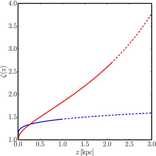
The importance of tilt, as quantified by equation (22). The blue and red lines correspond to tilt terms derived from the high- and low-metallicity population fits of Fig. 1. The deviation arising from the tilt term increases more rapidly with height for the low-metallicity population (red line), which probes the high-z region most useful for determining the DM profile. Dashed lines indicate extrapolation from data. For this case R0 = R1 = 2.5 kpc, and F = 267.65 km2 kpc−2 s−2.
Ignoring the tilt term will always cause an underestimation of the local DM density, if all other components of the model such as baryons are held steady. Looking at equation (21), we note that R0 < R⊙ and A > 0, meaning the tilt term |$\mathcal {T}(\mathrm{R}_{\odot }, z)$| is always negative. Then considering equation (3) we see that to fit to |$\sigma _z^2(z)$| in the absence of the tilt term |$\mathcal {T}(z^{\prime })$|, the Kz(z′) term, a negative term, is forced to become less negative in order to compensate. This requires a lower mass density, which, if the baryon density profile is held constant, manifests itself as a decrease in the DM mass density.
2.6 Statistical analysis and MultiNest
Assuming Gaussian errors it is possible to derive an empirical scale relating the Bayes factor to the strength of evidence for one model over another, as done in Trotta (2008). There, a |ln B01| value of less than 1 is considered inconclusive, while values of 1.0, 2.5 and 5.0 are considered to give weak, moderate and strong evidence, respectively.
Table 2 shows the prior ranges used for our analyses. We derive credible regions (CRs) for the DM density parameters by taking its posterior distribution and marginalizing over the remaining parameters. As outlined above our model has several components that can be turned on or off, such as the DD. Using the Bayesian evidence as calculated by MultiNest it is potentially possible to perform model comparison to determine which reconstruction model best fits the data. This idea will be explored in greater depth in subsequent studies.
Prior ranges for parameters. Gaussian priors are described by a median μ and a standard deviation |$\mathit {SD}$|. Note that ν(0) and σz(0) are the tracer density and velocity dispersion at z = 0, while quantities subscripted with 0, such as ν0 and |$\mathit {SD}_{\nu , 0}$|, are the values derived from data in the 0th bin, whose bin centre z0 > 0. Tracer density ν(0) has units of [stars kpc−3]. Kbn and KDD terms have units [km2 kpc−1 s−2].
| Model parameter | Range or Gaussian μ & SD | Type | |
|---|---|---|---|
| Baryons | Kbn | μ = 1500, |$\mathit {SD}=150$| | Gaussian |
| Dbn | μ = 0.18 kpc, |$\mathit {SD}=0.02$| kpc | Gaussian | |
| Constant DM | ρDM | [2, 20] × 10−3 M⊙ pc−3 | Linear |
| [0.076, 0.796] GeV cm−3 | |||
| DD | KDD | [0, 1500] | Linear |
| DDD | [1.5, 3.5] kpc | Linear | |
| Tilt term | A | [0, 200] km2 s−1 | Linear |
| n | [1.0, 1.9] | Linear | |
| R0 | μ = 2.5 kpc, |$\mathit {SD}=0.5$| kpc | Gaussian | |
| Tracer density | ν(0) | [0, ν0 + |$2\times \mathit {SD}_{\nu , 0}$|] | Linear |
| h | [0.4, 1.4] kpc | Linear | |
| Velocity disp. | σz(0) | [|$\sigma _{z,0} - 2 \times \mathit {SD}_{\sigma _z, 0}$|, | Linear |
| |$\sigma _{z,0} + 2\times \mathit {SD}_{\sigma _z, 0}$|] km s−1 | |||
3 MOCK DATA SETS
In this paper we apply our method only to mock data in order to hone and verify it. This mock data is ‘as good as it gets’, in the sense that it has no measurement errors, nor observational biases added to it, and is drawn from relatively simple, known distribution functions. While dynamically realistic ‘N-body’ mocks are preferred, it has already been shown that 1D Jeans analyses are robust to the presence of local non-axisymmetric structure in the disc (Garbari et al. 2011). Furthermore, N-body mocks are expensive; even state-of-the-art simulations do not approach the local sampling expected from Gaia. Finally, the expense of building well-sampled N-body mocks makes it challenging to explore a large parameter space of models, including models with and without tilt, or with and without a DD. For these reasons, we focus here on simpler mock data, similarly to the Read (2014) review. We will consider more dynamically realistic mocks, and mocks that give a faithful representation of the expected Gaia data uncertainties in future work.
We generate here a variety of mock data sets as outlined in Table 3, with different samplings (104, 105, and 106 tracer stars), with and without a tilt term, and also with either no DD, a DD (dd), or a more massive ‘big dark disc’ (bdd). We assume the axial term |$\mathcal {A}$| and the rotation curve term |$\mathcal {R}$| are zero. Our simple baryonic disc model is set up to mimic the real Milky Way, with a scale height parameter of Dbn = 0.18 kpc and a surface density of Σbn = 55.53 M⊙ pc−2, similar to those measured near the solar position (Flynn et al. 2006; Read 2014; McKee et al. 2015). The value of the F parameter (see equation 15) corresponds to a DM density of ρDM, const = 10 × 10−3 M⊙ pc−3 = 0.38 GeV cm−3. For each scenario we generate 20 mock data sets, allowing us to explore the effects of Poisson noise over a range of realizations.
Mock data parameters. _X is the number of stars sampled, e.g. 104, 105, 106, and _M is the mock number, ranging from 0 to 19. Empty spaces indicate that a certain mock data set does not include that element. The baryon model corresponds to a baryonic surface density of Σbn = 55.53 M⊙ pc−2, while the F parameter corresponds to a constant DM density of ρDM, const = 10 × 10−3 M⊙ pc−3 = 0.38 GeV cm−3. Kbn and KDD terms have units [km2 kpc−1 s−2], while F has units [km2 kpc−2 s−2].
 |
|
Mock data parameters. _X is the number of stars sampled, e.g. 104, 105, 106, and _M is the mock number, ranging from 0 to 19. Empty spaces indicate that a certain mock data set does not include that element. The baryon model corresponds to a baryonic surface density of Σbn = 55.53 M⊙ pc−2, while the F parameter corresponds to a constant DM density of ρDM, const = 10 × 10−3 M⊙ pc−3 = 0.38 GeV cm−3. Kbn and KDD terms have units [km2 kpc−1 s−2], while F has units [km2 kpc−2 s−2].
|
|
To derive the velocities for the mock catalogue we first must define a mass model and tilt. Taking the same parametrizations as described in Sections 2.3, 2.4, and 2.5 for baryons, DM, and tilt, respectively, we set their parameters as per Table 3. This allows us to calculate Kz and |$\mathcal {T}(z)$|. Using equation (5) and its associated assumptions we can calculate C. We then use equation (3) to derive σz(z). For each star we take its position z′, find the value of σz(z′), and then draw a velocity from a Gaussian centred on vz = 0 and with variance |$\sigma _z^2(z^{\prime })$|.
To generate vRvZ mock data, when necessary, we take the A, n, and R0 parameters listed in Table 3 and calculate the σRz(z) profile via equation (20). Taking each star's position z′, we calculate σRz(z′), and draw a value of vRvz from a Gaussian centred on vRvz = 0 and with variance of |$\sigma _{Rz}^2(z^{\prime })$|.
4 RESULTS
Here we present the results of our scans. We first investigate how the precision of the reconstruction varies with different numbers of tracer stars. We then look at the effects of the tilt term and the DD. For certain parts of these analyses the model used to generate the mock data and the model used to reconstruct the mock data are not the same – this is done to investigate the effects of ignoring terms (as in the case of the tilt term) or using incorrect models.
In the following figures we plot the marginalized posterior for the DM density ρDM(z), showing 68 per cent, 95 per cent, and 99.7 per cent CRs in dark, medium and light shading, respectively. The mock data profile is shown by the solid black line, while the median of the posterior distribution is shown by a solid line in the same colour as the CR. Binning of stars to calculate ν(z), σz(z), and σRz(z) is performed such that each bin contains an equal number of stars. For this study we use 20 bins, and in Appendix A we briefly explore the effects of changing the number of bins used. For plots with constant DM density in both mock data set and reconstruction model we plot all 20 mock data sets together, while for non-constant DM density in either mock or reconstruction we show one representative figure in this section, and show the full set of figures in Appendix B (Figs B1 to B6).
Our method and code is set up to describe the tracer density as a sum of exponentials. To determine the necessary number of exponentials required to describe the data we can use the Bayes factor as described earlier in Section 2.6. Test reconstructions give a Bayes factor of 1.5 when comparing one exponential to two, and 3.3 when comparing one exponential to three, with one exponential favoured in both cases. This is to be expected given that the mock data are generated using a single exponential. Given this result we use a single exponential for all subsequent reconstructions.
4.1 Sampling
Fig. 3 shows reconstructions of the local DM density for using varying numbers of tracer stars. The mock data sets used here are the most simple case, thick_X_M as described in Table 3, and has no DD or tilt added. As expected the CRs shrink as the number of tracer stars is increased from 104 stars up to 106 stars. The SDSS has sampling of the order of 104 stars (Zhang et al. 2013; Büdenbender et al. 2015) while data from Gaia will give upwards of 106 tracer stars.
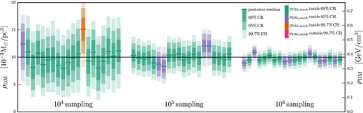
Determination of the DM density profile for varying numbers of tracer stars. These plots show marginalized posteriors for ρDM(z) = ρDM, const for the 20 mock data sets generated for each sampling level. Dark, medium, and light shading show the 68 per cent, 95 per cent, and 99.7 per cent CRs, respectively. Green, purple, and orange colouring indicates that the 68 per cent, 95 per cent, or 99.7 per cent CR, respectively, contains the correct answer. The median value of each posterior is shown by a solid line in green, purple, or orange, while the DM density value used to generate the mock data is shown as a solid black line across the entire plot. The mock data and reconstruction models used contain no tilt term or DD terms. As the number of tracer stars is increased from 104 to 106 the CRs for ρDM, const naturally shrink around the mock data value.
4.2 Tilt
In Fig. 4 we explore the effects of the tilt term. The left-hand set of CRs in Fig. 4 is the same as the right hand set of CRs from Fig. 3, with no tilt term in the mock data or reconstruction. In the centre set of Fig. 4, however, the mock data thick_tilt_1e6_M has the tilt term turned on, but the analyses are performed with the tilt term set to zero. This illustrates the danger of ignoring tilt as discussed earlier in Section 2.5: the reconstructions return narrow CRs, but as expected they systematically underestimate the value of ρDM, with the true ρDM lying outside even the 99.7 per cent CRs. This underestimation, however, is remedied by turning on the tilt term in the model, as shown in the right hand set CRs in Fig. 4, where the correct DM density is always at least within the 95 per cent CR. The inclusion of extra parameters to describe the tilt term does, however, increase the size of the CRs.
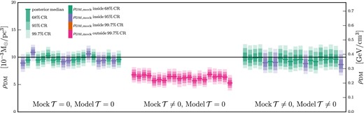
Determination of the DM density profile using 106 tracer stars and exploring the effects of including or neglecting the tilt term in the mock data sets and reconstruction models. These plots show marginalized posteriors for ρDM(z) = ρDM, const for the 20 mock data sets generated for each tilt scenario. Dark, medium, and light shading show the 68 per cent, 95 per cent, and 99.7 per cent CRs, respectively. Green, purple, and orange colouring indicates that the 68 per cent, 95 per cent, or 99.7 per cent CR, respectively, contains the correct answer, while pink colouring indicated that the correct answer lies outside even the 99.7 per cent CR. The median value of each posterior is shown by a solid line in green, purple, or orange, while the DM density value used to generate the mock data is shown as a solid black line across the entire plot. The left set of mocks shows the same result as the right set of Fig. 3, with no tilt term in mock data or reconstruction model. The centre set has a tilt term in the mock data but not in the reconstruction model, yielding a systemic underestimation of ρDM. The right set has a tilt term in both mock data and reconstruction model, demonstrating that our method can successfully deal with the tilt term.
Just as our determination of ρDM(z) is dependent on the tilt term, the tilt term is in turn dependent on its input parameters, A, n, and R0 = R1. While we have been able to fit for A and n using G-type dwarf data (Section 2.5), for R0 we have taken the canonical value of R0 = 2.5 ± 0.5 kpc from Binney & Tremaine (2008), and further made the assumption that σRz(R, z) has the same radial profile as ν(R, z) (i.e. R0 = R1). When using only a single population, determination of R0 and R1 will be important, as illustrated in Fig. 5. This figure shows the 2D marginalized posterior for ρDM, const and R0 for a reconstruction of mock data set thick_tilt_1e6_0 with a model including tilt, and demonstrates the degeneracy that exists between ρDM, const and R0 = R1. If using multiple tracer population, each will have different R0 and/or R1, but will all have their motions dictated by the same potential. This will help us break the degeneracy between R0, R1, and ρDM. Further, with the advent of Gaia data we will be able to directly measure the radial profile of σRz and ν(R, z) for a given set of tracer stars.
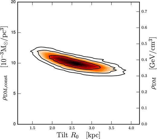
2D marginalized posterior of the constant DM density ρDM(z) = ρDM, const and the R0 parameter of the tilt term (equation 19), generated from mock data set thick_tilt_1e6_0 reconstructed using a model with tilt. Contours show the 68 per cent, 95 per cent, and 99.7 per cent CRs. Marginalization and plotting performed using Barrett (Sebastian Liem, private communication).
4.3 Dark disc
Fig. 6 shows mock data set thick_1e6_0-19, thick_dd_1e6_0, and thick_bdd_1e6_0 reconstructed using models with and without a DD component. The top left panel shows the same CRs as seen in the left hand set of Fig. 4 and the right hand set of Fig. 3.
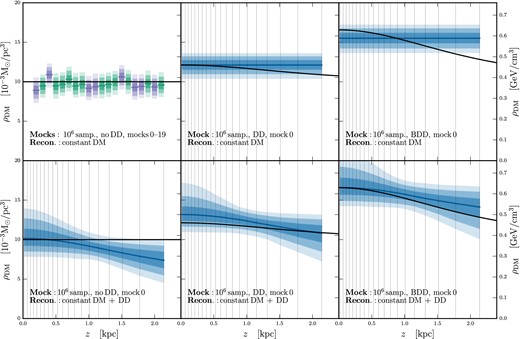
Determination of the DM density profile using 106 tracer stars and exploring the effects of including or neglecting a DD in the mock data sets and reconstruction models. For comparison the top left panel shows the same reconstructions as the right hand set from Fig. 3, i.e. basic mock data sets with no DD, reconstructed with a constant DM density. The remaining panels each show one representative mock and reconstruction, with the full set of mocks and reconstructions given in Appendix B. These panels show marginalized posteriors for ρDM(z), with dark, medium, and light shading indicating the 68 per cent, 95 per cent, and 99.7 per cent CRs, respectively. The median value of the posterior is shown by the solid blue line, while the DM density profile used to generate the mock data is shown as a solid black line. From left to right the columns show reconstructions of mock data sets containing no DD (ρDM, const only), a DD, or a ‘big’ dark disc (BDD). The top centre and top right panels show the determination of a constant DM density from the DD and BDD mock data sets, respectively. The bottom row shows the reconstruction of each of the mock data sets using a model with a constant DM term and a DD term. Light grey vertical lines indicate the bin centres.
The left column of Fig. 6 shows the reconstruction of mock data sets with a constant DM density profile: mocks 0–19 in top left and mock 0 in bottom left. The reconstruction in the top panel uses a model with a constant DM density, while the bottom panel uses a model with an additional DD component. The DD reconstruction exhibits a disc structure even though the correct answer is constant ρDM. This is likely due to a bias in the hyper-volume set by the priors – the prior range on the DD parameters goes between no DD (KDD = 0) and a maximal DD (KDD = 1500), and thus the bulk of the parameter space features at least some DD. There is no ‘negative dark disc’ to counteract this effect and push the mean of the prior range back to no DD.
In the centre and right columns of Fig. 6 we reconstruct mock data sets with a DD of different masses: thick_dd_1e6_0 and thick_bdd_1e6_0 (the ‘big dark disc’). A constant DM density reconstruction (top row) is able to contain the thick_dd_1e6 DD within the 95 per cent CR almost to the last bin, but fails to contain the big dark disc beyond z = 1.3 kpc. Adding a DD term allows the reconstruction to fit to the mock data DM profile nicely, as shown in the bottom centre and bottom right panels of Fig. 6.
When working with real data, however, we will not have the luxury of knowing the DM profile underlying the data. The black mock data model line will not be there. In subsequent studies we will explore the potential use of the Bayesian evidence, as calculated by MultiNest, to determine if a DD is justified by observational data.
4.4 Tilt and dark disc
Here, we combine the two elements discussed in previous sections, the tilt term and the DD. Fig. 7 shows reconstructions of the mock data set thick_bdd_tilt_1e6_0. In the top panel the reconstruction model contains neither DD nor tilt term. Again, we see the same effects as we did previously. The missing tilt term yields a consistent underestimation of the DM density, and the constant DM density envelope is too narrow to encompass the density range of the DD. The consistent underestimation can be remedied by adding a tilt term to the reconstruction model, as shown in the middle panel, where the reconstruction model has a tilt term included. Both problems can be resolved in tandem by using a reconstruction model with both tilt and DD terms, as shown in the bottom panel of Fig. 7.
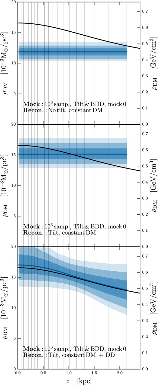
Determination of the DM density profile using 106 tracer stars with a combination of a tilt term and a DD in the mock data (thick_bdd_tilt_1e6_0) and using a variety of reconstruction models. These plots show marginalized posteriors for ρDM(z), with dark, medium, and light shading indicating the 68 per cent, 95 per cent, and 99.7 per cent CRs, respectively. The median value of the posterior is shown as the solid blue line, while the DM density profile used to generate the mock data is shown as a solid black line.
5 CONCLUSIONS
In this paper we have presented a new method of determining the vertical DM density profile, and thus the local DM density. The key equation of this method, equation (3), depends only on the assumption of dynamical equilibrium. In practice, further assumptions are made to describe the components going in to equation (3); however the scope of possible models is wide, and in principle model selection using the Bayesian evidence can be used to determine the best model. We leave exploration of this last aspect to future work.
The importance of the tilt term has been previously noted (Kuijken & Gilmore 1989a; Smith et al. 2009; Büdenbender et al. 2015), and to derive an accurate value for the local DM density it is vital that our method be able to deal with this term. The baryonic contribution to the galactic density profile drops rapidly as z increases, leaving DM as the dominant component. Thus to probe the DM density profile sampling thick disc stars that travel higher above the plane are preferable. For these populations the tilt term is more important, as illustrated in Fig. 2. Failure to include the tilt term in the analysis leads to a systematic underestimation of the local DM density, as explained in Section 2.5 and demonstrated in Section 4.2.
One of the novel aspects of our method is that it can deal with the tilt term while remaining within the confines of the one-dimensional z-direction Jeans equation, which can be seen in Fig. 4. With only the data currently available for the Milky Way, this requires several well-motivated assumptions, as described in Section 2.5. However, with data from Gaia we will be able to directly measure the radial profile of the tilt and tracer density, removing the need for such assumptions. While for this paper we have disregarded the rotation curve term (equation 6), we note that an accurate determination of this will be necessary for the implementation of this or other z-direction methods to real data.
Non-spherical DM density profiles, such as oblate haloes or accreted DDs, can also be fitted using our method by incorporating a DD term into the reconstruction model, which is shown in Fig. 6. Our method can also reconstruct mock data sets containing both a tilt term and a DD, as shown in Fig. 7.
We thank Michael Feyereisen, Sebastian Liem, Pat Scott, Roberto Trotta, Stephen Feeney, Roberto Ruiz de Austri, Scott Tremaine, Vera Gluscevic, and Juna Kollmeier for very useful discussions. SS acknowledges support from the Swedish Research Council (VR, Contract No. 350-2012-268). JIR would like to acknowledge support from STFC consolidated grant ST/M000990/1 and the MERAC foundation. GB acknowledges support from the European Research Council through the ERC starting grant WIMPs Kairos.
In the context of the values of the prior ranges given in Table 2, the gravitational constant equals |$G = 4.229\times 10^{-6}\, {\rm km}^2\, {\rm kpc}\, {\rm M}_{\odot }^{-1}\, {\rm s}^{-2}$|.
Private communication with authors.
REFERENCES
APPENDIX A: VARIATION DUE TO THE NUMBER OF BINS
Fig. A1 illustrates the effects of changing the number of bins used for this analysis. There we plot the 68 per cent, 95 per cent, or 99.7 per cent CRs for 20 mock data sets (thick_1E6_0-19, no tilt and no DD), and vary the number of bins from five to 30, in increments of five. For only five bins (top left set), the true answer for ρDM, const is outside the 99.7 per cent CR for all but two of the mocks, for which the true answer is within only the 99.7 per cent CR. The systematic underestimation is due to an overestimation of the baryonic disc. The fifth bin in this scheme covers a range from 1.2 to 2.4 kpc and has its bin centre at z = 1.6 kpc, so it is unsurprising that such a low number of bins fail to correctly reconstruct the DM profile, which is a subdominant component, only becomes apparent at higher z. Increasing the number of bins to 10, 15, and then to 20 improves the results. The gains from increasing from 20 to 25 and 30 bins are very slight.
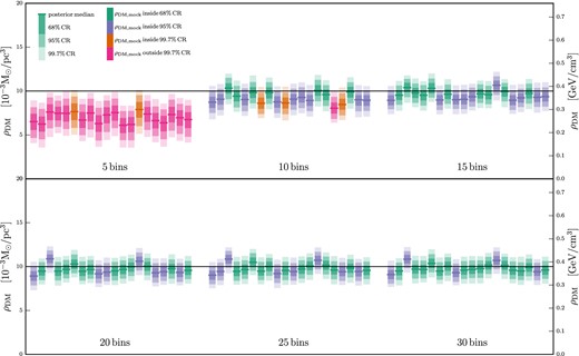
Exploring the effects of binning on the determination of ρDM. These plots show marginalized posteriors for ρDM(z) = ρDM, const for the 20 mock data sets thick_1E6_0-19, reconstructed using 5, 10, 15, 20, 25, and 30 bins. Dark, medium, and light shading show the 68 per cent, 95 per cent, and 99.7 per cent CRs, respectively. Green, purple, and orange colouring indicates that the 68 per cent, 95 per cent, or 99.7 per cent CR, respectively, contains the correct answer, while pink colouring indicated that the correct answer lies outside even the 99.7 per cent CR. The median value of each posterior is shown by a solid line in green, purple, or orange, while the DM density value used to generate the mock data is shown as a solid black line across the entire plot.
APPENDIX B: Dark Disc Reconstructions with Multiple Mocks
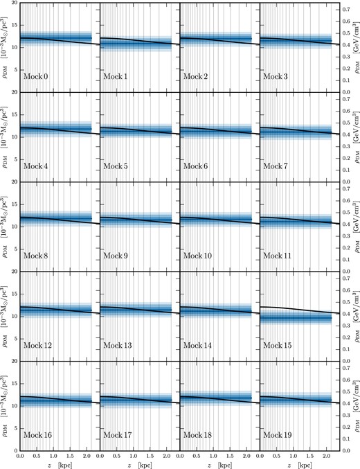
Here we show the results of reconstructing all mocks data sets generated using a constant DM density only (thick_X_M), constant DM and a regular DD (thick_dd_X_M), or constant DM and a ‘big’ DD (thick_bdd_X_M) (see Table 3 for details). The reconstruction models either have a constant DM density only or a constant DM density plus a DD.
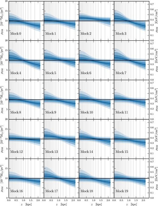
Marginalized posteriors of ρDM(z) for mock data sets thick_1E6_0-19 with ρDM, const only (no DD component) reconstructed using a model with ρDM, const plus a DD. Dark, medium, and light shading indicate the 68 per cent, 95 per cent, and 99.7 per cent CRs, respectively. The median value of the posterior is shown as the solid blue line, while the DM density profile used to generate the mock data is shown as a solid black line.
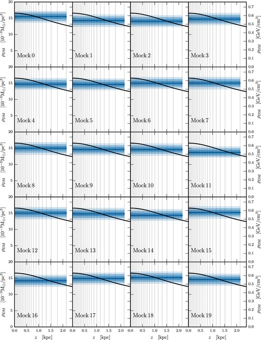
Marginalized posteriors of ρDM(z) for mock data sets thick_dd_1E6_0-19 with ρDM, const plus a DD component, reconstructed using a model with ρDM, const only. Dark, medium, and light shading indicate the 68 per cent, 95 per cent, and 99.7 per cent CRs, respectively. The median value of the posterior is shown as the solid blue line, while the DM density profile used to generate the mock data is shown as a solid black line.

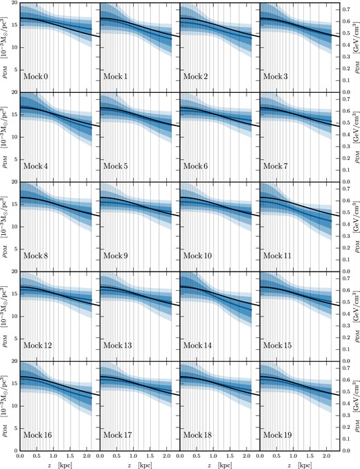
Marginalized posteriors of ρDM(z) for mock data sets thick_dd_1E6_0-19 with ρDM, const plus a DD component, reconstructed using a model with ρDM, const and a DD component. Dark, medium, and light shading indicate the 68 per cent, 95 per cent, and 99.7 per cent CRs, respectively. The median value of the posterior is shown as the solid blue line, while the DM density profile used to generate the mock data is shown as a solid black line.
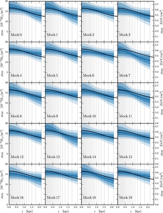
Marginalized posteriors of ρDM(z) for mock data sets thick_bdd_1E6_0-19 with ρDM, const plus a DD component, reconstructed using a model with ρDM, const only. Dark, medium, and light shading indicate the 68 per cent, 95 per cent, and 99.7 per cent CRs, respectively. The median value of the posterior is shown as the solid blue line, while the DM density profile used to generate the mock data is shown as a solid black line.
Marginalized posteriors of ρDM(z) for mock data sets thick_bdd_1E6_0-19 with ρDM, const plus a ‘big’ DD component, reconstructed using a model with ρDM, const and a DD component. Dark, medium, and light shading indicate the 68 per cent, 95 per cent, and 99.7 per cent CRs, respectively. The median value of the posterior is shown as the solid blue line, while the DM density profile used to generate the mock data is shown as a solid black line.
Marginalized posteriors of ρDM(z) for mock data sets thick_bdd_tilt_X_0-19 with ρDM, const plus a ‘big’ DD component and including the effects of tilt, reconstructed using a model with ρDM, const, a DD component, and incorporating tilt. Dark, medium, and light shading indicate the 68 per cent, 95 per cent, and 99.7 per cent CRs, respectively. The median value of the posterior is shown as the solid blue line, while the DM density profile used to generate the mock data is shown as a solid black line.
