


Abstract
Previous works have clearly shown the existence of winds from black hole hot accretion flow and investigated their detailed properties. In extremely low accretion rate systems, the collisional mean-free path of electrons is large compared with the length-scale of the system, thus thermal conduction is dynamically important. When the magnetic field is present, the thermal conduction is anisotropic and energy transport is along magnetic field lines. In this paper, we study the effects of anisotropic thermal conduction on the wind production in hot accretion flows by performing two-dimensional magnetohydrodynamic simulations. We find that thermal conduction has only moderate effects on the mass flux of wind. But the energy flux of wind can be increased by a factor of ∼10 due to the increase of wind velocity when thermal conduction is included. The increase of wind velocity is because of the increase of driving forces (e.g. gas pressure gradient force and centrifugal force) when thermal conduction is included. This result demonstrates that thermal conduction plays an important role in determining the properties of wind.
1 INTRODUCTION
Hot accretion flow such as advection-dominated accretion flow (Narayan & Yi 1994, 1995; Abramowicz et al. 1995) is interesting because it can be used to model the low-luminosity active galactic nuclei (LLAGNs), which are the majority of galaxies at least in the nearby universe, and the hard/quiescent states of black hole X-ray binaries (see Yuan & Narayan 2014 for the latest review of current theoretical understanding of hot accretion flow and its various astrophysical applications).
Numerical simulations of hot accretion flow show that the mass inflow rate (see equation 7 for definition) decreases with decreasing radius |$\dot{M}_{\rm in} (r) \propto r^s$| with s ∼ 0.5–1 (e.g. Stone, Pringle & Begelman 1999; Igumenshchev & Abramowicz 1999, 2000; Hawley & Balbus 2002; Pang et al. 2011; Yuan, Wu & Bu 2012a; Bu et al. 2013). Especially Yuan, Bu & Wu (2012b) show that the inward decrease of the accretion rate is due to the significant mass-loss via wind (see also Narayan et al. 2012; Li, Ostriker & Sunyaev 2013). This conclusion is soon confirmed by the 3.0 × 10⁶ s Chandra observations of the accretion flow around the supermassive black hole in the Galactic Centre, combined with the modelling to the detected iron emission lines (Wang et al. 2013). Begelman (2012) and Gu (2015) address the question of why wind exists. The detailed properties of wind such as the mass flux, angular distribution, terminal velocity, and fluxes of energy and momentum, have been studied in Yuan et al. (2015, see also Sadowski et al. 2016) by following the trajectories of the fluid particles. Bu et al. (2016) show that wind production can only occur within the Bondi radius of the accretion flow.
All the simulations mentioned above have neglected the effects of thermal conduction. However, thermal conduction is very important when the accretion rate is very low. In low accretion rate systems, the electron mean-free path is very large. In this case, thermal conduction can have a significant influence on the dynamics of the accretion flow (Quataert 2004; Johnson & Quataert 2007), resulting in the transport of thermal energy from the inner (hotter) to the outer (cooler) regions. If the energy flux carried by thermal conduction is substantial, the temperature of the gas in the outer regions can be increased above the virial temperature. Thus, gas in the outer regions is able to escape from the gravitational potential of the central black hole and form outflows, significantly decreasing the mass accretion rate (Tanaka & Menou 2006; Johnson & Quataert 2007; Abbassi, Ghanbari & Najjar 2008; Sharma, Quataert & Stone 2008; Ghanbari, Abbassi & Ghasemnezhad 2009; Bu, Yuan & Stone 2011; Ghasemnezhad, Khajavi & Abbassi 2012).
If the mean-free path of electron is much larger than its gyro-radius, conduction will be anisotropic and along magnetic field lines (Balbus 2000, 2001; Parrish & Stone 2005, 2007; Quataert 2008; Foucart et al. 2016). In many LLAGNs, the electron mean-free path is much larger than electron gyro-radius (see Tanaka & Menou 2006). Let us take the accretion flow in Galactic Centre as an example to compare the electron mean-free path to their gyro-radius. From Chandra observations of the accretion flow at the Galactic Centre, Sgr A*, the electron mean-free path is estimated to be 0.02–1.3 times the Bondi radius, i.e. the electron mean-free path l ∼ 1.3 × 1017cm (Tanaka & Menou 2006). The gyro-radius of electrons is |$R_{\rm gyro}=m_{\rm e} v_{\rm {th}} c/qB \sim 4\times 10^5\sqrt{\beta /n}$|, where me is electron mass, vth is thermal speed of electron, c is speed of light, q is electron charge, B is magnetic field, β is the ratio between gas pressure and magnetic pressure, and n is number density of electrons. At 105Rs, n = 100, Rgyro ∼ 105cm if we assume β ∼ 10; Therefore, it is clear that electron mean-free path is much larger than its gyro-radius. For the accretion flow at Galactic Centre n ∼ r−1/2, so Rgyro ∝ r1/4 if we assume β is almost constant in the accretion flow. But the electron mean-free path l ∝ r−3/2 (Tanaka & Menou 2006). As a result, the electron mean-free path will become even larger than gyro-radius when approaching the central black hole event horizon.
In this paper, we study the effects of anisotropic thermal conduction on the properties of hot accretion flow by performing two-dimensional magnetohydrodynamic (MHD) simulations. We especially pay attention to the wind properties, such as the mass, momentum, and energy fluxes of wind launched from the accretion flow. These quantities are essential for the study of active galactic nucleus feedback since winds play an important role in the feedback process. For example, the two gamma-ray Bubbles observed by the Fermi-LAT below and above the Galactic plane (Su, Slatyer & Finkbeiner 2010) may be inflated by the wind from the hot accretion flow in our Galactic Centre (Mou et al. 2014). In Section 2, we will describe the basic equations and the simulation method. In Section 3, we will present the results. We discuss and summarize our results in Section 4.
2 NUMERICAL METHOD AND MODELS
2.1 Numerical method
The final terms in equations (3) and (4) are the magnetic heating and dissipation rate mediated by a finite resistivity η. Since the energy equation here is actually an internal energy equation, numerical reconnection inevitably results in loss of energy from the system. By adding the anomalous resistivity, the energy loss can be captured in the form of heating in the current sheet (Stone & Pringle 2001). The exact form of η is same as that used by Stone & Pringle (2001).
We use the pseudo-Newtonian potential to mimic the general relativistic effects, Φ = −GMBH/(r − Rs), where G is the gravitational constant and MBH is the mass of the central black hole. The self-gravity of the gas is neglected. In this paper, we set GMBH = Rs = 1. We use Rs to normalize the length-scale. Time is in unit of the Keplerian orbital time at 100Rs. The black hole in our Galactic Centre has a mass MBH ≈ 4 × 10⁶M⊙, M⊙ is the solar mass. For the black hole in our Galactic Centre, the length unit (Rs) is ∼1012 cm. The orbital time at 100Rs is ∼3.8 × 10⁵ s.
Following Sharma et al. (2008), we assume κ = χT/p which has the dimensions of a diffusion coefficient (cm2 s− 1). In non-relativistic theory, |$\kappa \propto c_{\rm s}^2 \tau _{\rm R}$|, with cs is the sound speed and τR is the effective mean-free-time due to wave-particle scatterings (Foucart et al. 2016). A nature scale for τR is the dynamical time |$\sqrt{r^3/(G M_{\rm BH})}$|. For the hot accretion flow such as Sgr A*, the temperature of gas is almost virial; therefore, the sound speed is proportional to the Keplerian rotational velocity cs ∝ vk ∝ r−1/2. Thus, for hot accretion flow, κ ∝ r1/2. In this paper, we assume that κ ≡ αc(GMBHr)1/2. The precise value of αc, which depends on the microphysical processes, is difficult to calculate. Motivated by the results of Sharma et al. (2006) and Sharma, Quataert & Stone (2007) on the microphysics in collisionless accretion flows, we take αc = 0.2. This value is much smaller than the maximum free-streaming thermal conductivity that could be obtained if the electrons are virial.
2.2 Initial conditions and numerical settings
The computational domain is from Rin = 1.3 or 2Rs to Rout = 400Rs in radial direction and from θ = 0° to θ = 180° in angular direction. The radial grids are logarithmically spaced (grid spacing dr ∝ r). In angular direction, the grids are uniformly spaced. The axisymmetric boundary conditions are used at θ = 0° and 180°. We adopt outflow boundary conditions at both the inner and outer radial boundaries. The standard resolution is 147 × 88. Several modifications to the code were required for the simulations, including implementing the pseudo-Newtonian potential, adding the anomalous resistivity and thermal conduction. The thermal conduction is implemented by using the method based on limiters (Sharma & Hammett 2007), this method can guarantee the heat always flows from hot regions to cold regions.
2.3 Models
Due to the fact that thermal conduction is transported along magnetic field lines, if the magnetic field is much ordered, we expect energy can be transferred from inner to outer region which will affect the dynamics of the flow significantly. If the magnetic field is much tangled, we expect the energy cannot be transferred to large distance which may result in small effects on the dynamics of the flow. Motivated by this point, we explore two different magnetic configurations: a large-scale ordered magnetic field and a relative small-scale tangled magnetic field to examine the effects of thermal conduction on hot accretion flow.
The magnetic field which threads the torus initially is generated by a vector potential, i.e. |${\boldsymbol B}=\nabla \times \boldsymbol A$|. Initializing the field in this way guarantees that it will be divergence free. We take |$\boldsymbol A$| to be purely azimuthal. In model A series, we assume |$\boldsymbol A_\phi =\rho ^2/\beta _0$| and β0 = 100. This will generate a dipolar field (see the left-hand panel of Fig. 1). With the value of β0 = 100, when the flow achieves steady state, the field is much ordered. In model B series, we assume the field is quadrupolar with |$\boldsymbol A_\phi =\rho ^2/\beta _0 r \cos \theta$| (see the right-hand panel of Fig. 1). For the quadrupolar field, the magnetic loops below and above the equatorial plane have opposite polarity. Thus, magnetic reconnection is very strong and finally the magnetic field is prone to be tangled.
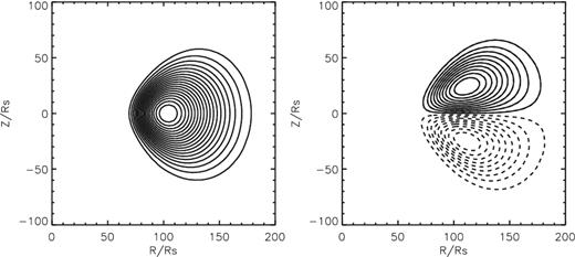
Initial magnetic field configurations for model A series (left-hand panel) and B series (right-hand panel). Solid and dashed lines indicate field polarity: solid lines denote current into the page, dashed lines denote current out of the page.
Table 1 lists the main parameters in all models presented here, initial magnetic field topology, plasmas parameter β0, thermal conductivity αc, and final time tf at which each simulation is stopped (all times in this paper are reported in units of the orbital time at R0 = 100Rs.)
Simulation parameters.
| Name | Field topology | αc | β0 | |$t_{f}^a$| |
|---|---|---|---|---|
| A0 | dipole | 0 | 100 | 4 |
| A1 | dipole | 0.2 | 100 | 4 |
| B0 | quadrupole | 0 | 50 | 10 |
| B1 | quadrupole | 0.2 | 50 | 10 |
| Name | Field topology | αc | β0 | |$t_{f}^a$| |
|---|---|---|---|---|
| A0 | dipole | 0 | 100 | 4 |
| A1 | dipole | 0.2 | 100 | 4 |
| B0 | quadrupole | 0 | 50 | 10 |
| B1 | quadrupole | 0.2 | 50 | 10 |
Note.aFinal time at which each simulation is stopped (all times in this paper are reported in units of the orbital time at R0 = 100Rs.).
3 RESULTS
In numerical simulations, the net mass accretion rate (see equation 9) is always used as a diagnostic to see whether a quasi-steady state is achieved (e.g. Stone et al. 1999). If a quasi-steady state is achieved, the net mass accretion rate is almost a constant of radius. From Fig. 2 (dotted lines), we can see that the net mass accretion rate is almost a constant of radius. Therefore, the simulations in this paper have reached a quasi-steady state. In the MHD simulations, there is turbulence induced by the magneto-rotational instability (MRI). Therefore, the physical quantities always vary with time around their mean values. As an example, Fig. 3 shows the mass flux of outflow at r = 20Rs in model A1. It is clear that after t = 1.2 orbits, a quasi-steady state is achieved, the mass flux of outflow oscillates with very small amplitude around its mean value.
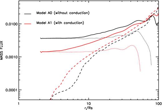
The radial profiles of the time-averaged (from t = 1.5 to 1.6 orbits) and angle-integrated mass inflow rate |$\dot{M}_{\rm in}$| (solid line), outflow rate |$\dot{M}_{\rm out}$| (dashed line), and the net rate |$\dot{M}_{\rm acc}$| (dotted line) in model A0 (black lines) and A1 (red lines).
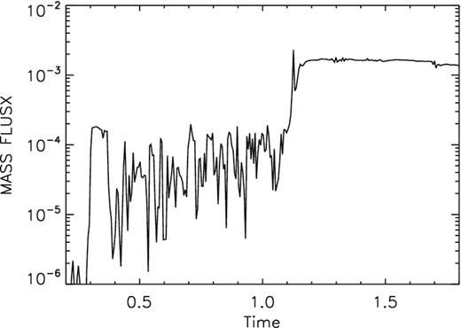
Time evolution of the mass outflow rate at r = 20Rs calculated by equation (8) in model A1.
3.1 Dipolar field models
At first we analyse model A series, all the data are time averaged from t = 1.5 to 1.6 orbits except the snapshot data is at time t = 1.6 orbits. Fig. 2 shows the radial profiles of the time-averaged mass inflow rate |$\dot{M}_{\rm in}$|, outflow rate |$\dot{M}_{\rm out}$|, and net rate |$\dot{M}_{\rm acc}$| in model A0 (without thermal conduction, αc = 0.0) and A1 (with thermal conduction, αc = 0.2). From this figure, it is clear that the mass inflow rate in both models decreases inwards, consistent with those found in previous works (see review in Yuan et al. 2012a). The mass inflow rate in model A1 decreases much quicker towards the black hole than model A0 and the net mass accretion rate in model A1 is about half of that in model A0. This is because the mass outflow rate in model A1 is larger than that in model A0. Note that we count all the gas with positive velocity as the mass outflow rate (see equation 8), i.e. the mass outflow rate includes both real outflow (wind) and gas which is doing turbulent motions. Thus the crucial issue to quantitatively study the strength of wind is to get rid of the contamination of turbulence. This is achieved in Yuan et al. (2015) by using a trajectory approach. Based on the general relativistic magnetohydrodynamic (GRMHD) simulation data of hot accretion flow (without thermal conduction), they convincingly show that the mass flux of real outflow is ∼60 per cent of the outflow rate calculated by equation (8).
While it is essential to use the trajectory approach to calculate the properties of wind such as the mass flux, as shown by Yuan et al. (2015), this approach is technically complicated and the calculation is very time-consuming. Since the aim of this work is to investigate the effect of thermal conduction, to qualitatively understand the above-mentioned different results between models A0 and A1, we find it is enough to simply use the time-averaged method often adopted in literature. The time-averaged density contour and velocity field are shown in Fig. 4. This figure shows the distribution of density contour overplotted by the poloidal velocity field within R = 20 Rs of models A0 (left-hand panel) and A1 (right-hand panel). In both models, the flow has two components: low-temperature high-density main disc body around the equator and high-temperature low-density corona sandwiching it. The main disc body is the inflow region (Sadowski et al. 2013; Yuan et al. 2015). We find that the wind region in model A1 is larger than that in model A0. For example, in model A0, it is inflow in the regions 26° < θ < 45° and 135° < θ < 154°. But in model A1, gas in these two regions becomes wind. The broader wind region in model A1 results in stronger wind and more rapid inward decrease of the inflow rate.
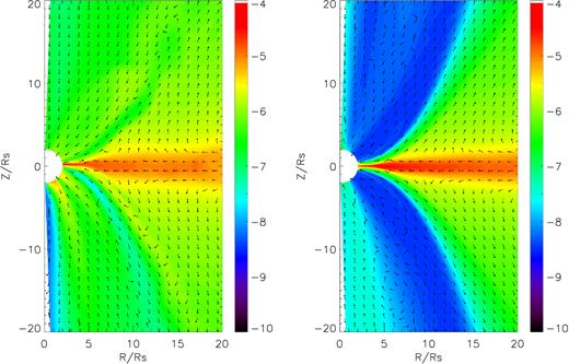
Time-averaged (from t = 1.5 to 1.6 orbits) density and velocity. Colours show the logarithm density. Arrows show the direction of velocity (|$\boldsymbol v/|\boldsymbol v|$|). The left-hand panel is for model A0 (without conduction). The right-hand panel is for model A1 (with conduction).
In order to figure out why the inflowing gas becomes wind, we plot magnetic field, heat flux, and temperature in Fig. 5. In Fig. 5, upper-left panel shows the snapshot of logarithm plasma β and magnetic field lines for model A1. Black lines are magnetic field lines; colours show logarithm plasma β. Upper-right panel shows the snapshot of conduction energy flux |$\boldsymbol Q$| and its divergence for model A1; colours show the divergence of conduction flux |$\nabla \cdot \boldsymbol Q$| for model A1. Arrows show the energy flux. Orange denotes regions those are heated by thermal conduction; green denotes regions those are cooled by thermal conduction. Bottom panels show the time-averaged (from t = 1.5 to 1.6 orbits) logarithm temperature for models A0 (left) and A1 (right), respectively. In model A series, because of a relative small plasma β and dipolar configuration field as the initial condition, the wavelength of the MRI (Balbus & Hawley 1991, 1998) is large which suppressed the turbulence driven by the MRI. Thus, the magnetic field evolves to a relative strong and ordered magnetic field as the upper-left panel of Fig. 5 shows. The thermal conduction flux is mainly along magnetic field lines, so it is also become very ordered. Heat energy is transferred from inner to outer region by thermal conduction. At the equator, the heat is transport from inner to larger radius and plays a cooling role. It is clear that gas in the regions 26° < θ < 45° and 135° < θ < 154° is heated up by the conduction flux along magnetic field lines. The increase of temperature in those regions results in the increase of gas pressure gradient force. Consequently, the increased gas pressure gradient force makes the inflowing gas changing moving direction and becoming wind. From the energy point of view, the Bernoulli parameter of the gas in these two regions becomes larger due to thermal conduction thus the gas is easier to become wind. This argument of wind production is similar to that presented in Gu (2015).
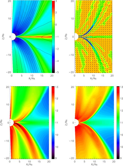
Upper-left panel shows the snapshot of logarithm plasma β = pgas/pmag (colours) and magnetic field lines (solid line) of model A1. Upper-right panel shows the snapshot of unit vector of conduction energy flux |$\boldsymbol Q / |\boldsymbol Q|$| (arrows) and divergence of conduction flux |$\nabla \cdot \boldsymbol Q$| (colours) of model A1, note that orange colour denotes region where gas is heated by thermal conduction and green colour denotes region where gas is cooled by thermal conduction. Bottom panels show the time-averaged logarithm temperature for models A0 (left) and A1 (right).

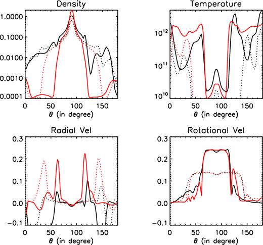
Angular profiles of a variety of time-averaged variables of model A0 (black lines, without conduction) and A1 (red lines, with thermal conduction) at r = 10Rs (solid lines) and 50 Rs (dotted lines). From left to right, upper to bottom, the panels denote the density, temperature, radial velocity, and angular velocity, respectively.
To figure out the reason of why the velocity of wind increases after the inclusion of thermal conduction, we calculate the forces exerting on gas. Based on the GRMHD simulation data, Yuan et al. (2015, see also Moller & Sadowski 2015) have shown that the wind is mainly driven by the centrifugal force, the gradient force of gas pressure and magnetic pressure. Fig. 8 plots the driving force for wind at θ = 65° and |$r=10R_{\rm {\rm s}}$| in model A0 (upper panel) and A1 (lower panel). In the case of model A0, the main driving forces are the combination of the gradient force of magnetic pressure and the gas pressure and the centrifugal force. It is clear that after the thermal conduction is included the gas pressure gradient force increases due to the increase of temperature. The magnetic pressure gradient force also increases. The increase of forces results in the larger velocity of wind in model A1 compared with A0.
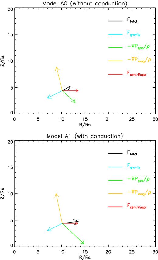
Force analysis at r = 10Rs and θ = 65° for model A0 (upper-panel) and A1 (lower-panel). The arrows indicate force direction, whose length represents force magnitude. All the forces are scaled in the same way, the scaled factor chosen arbitrarily to fit the arrows in both models.
3.2 Quadrupolar field models
In model A series, the magnetic field is strong and ordered. Therefore, thermal conduction along magnetic field can transport energy from the inner to outer region and affects the wind production significantly. If the magnetic field is tangled, one may expect that energy cannot be transferred to large distance. In this case, the effects of conduction may be smaller compared with the case when the magnetic field is ordered. In order to examine this point, we carry out model B series (see Table 1). In this series, the initial magnetic field configuration is quadrupolar (see the right-hand panel of Fig. 1). In this case, magnetic reconnection very easily occurs, which can decrease the strength of magnetic field. In this section, the data are usually time averaged from t = 3.0 to t = 3.5 orbits, except for the snapshot data is at time t = 3.5 orbits.
Fig. 9 shows the snapshot of logarithm of β overplotted with magnetic field lines (left-hand panel) and the unit vector of conduction energy flux |$\boldsymbol Q / |\boldsymbol Q|$| overplotted with the divergence of conduction flux |$\nabla \cdot \boldsymbol Q$| (right-hand panel) of model B1. Recall that in model A series, the magnetic field is ordered and the heat flux is transported mainly along the magnetic field lines so the heat flux is also ordered as seen in the upper-right panel of Fig. 5. But the case is different in model B series. Because the magnetic field is weaker and tangled, as shown in Fig. 9 (left-hand panel, solid line), the conduction energy flux (right-hand panel, arrows) is thus not ordered. Fig. 10 shows the mass accretion rates in model B series. It is clear that the mass accretion rates are only slightly changed after thermal conduction is taken into account. In order to study the reason, we plot the angular profiles of some quantities in Fig. 11. As shown in the upper-right panel, the angular profiles of temperature in model B1 is flatter than that in model B0, consistent with that found in Johnson & Quataert (2007). Except for the changes of density and temperature, the radial and rotational velocities of wind are also changed when considering thermal conduction. Now, we make a quantitative analysis of the changes of wind mass fluxes based on the changes of density and velocity of wind in model B1. Taking the physical values for wind at 10Rs as an example, wind is present at θ = 30° in model B0 and θ = 20° in model B1. When conduction is included, the velocity of wind increases but the density of wind decreases. So the mass flux of wind is just slightly decreased by a factor of ∼2.
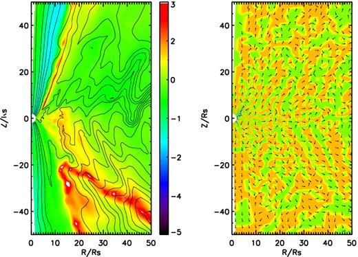
Left-hand panel shows the snapshot of logarithm plasma β and magnetic field lines for model B1. Black lines are magnetic field lines; colours show logarithm plasma β. The right-hand panel shows the unit vector of conduction energy flux |$\boldsymbol Q / |\boldsymbol Q|$| (arrows) and the divergence of conduction flux |$\nabla \cdot \boldsymbol Q$| (colours) for model B1. Note that in right-hand panel, orange colour denotes region which gas is heated by thermal conduction; green colour denotes region which gas is cooled by thermal conduction.
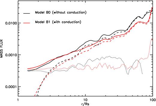
The radial profiles of the time-averaged and angle-integrated mass inflow rate |$\dot{M}_{\rm in}$| (solid line), outflow rate |$\dot{M}_{\rm out}$| (dashed line), and the net rate |$\dot{M}_{\rm acc}$| (dotted line) in model B0 (black lines) and B1 (red lines).

Angular profiles of a variety of time-averaged variables for model B0 (black lines, without conduction) and B1 (red lines, with thermal conduction) at r = 10Rs (solid lines) and 50 Rs (dotted lines).
Fig. 12 shows the energy and momentum fluxes carried by wind. It is clear that the momentum flux of wind is just slightly changed when thermal conduction is included. But the energy flux increases by a factor of ∼2. This is because that the momentum and energy fluxes of wind are |$\dot{P}_{{\rm wind}} \propto \rho v_r^2$| and |$\dot{E}_{{\rm wind}} \propto \rho v_r^3$|, respectively. In model B series, when conduction is included, the density of wind is decreased by a factor of ∼5 and velocity of wind is increased by a factor of ∼2. Therefore, the momentum flux is almost unchanged but the energy flux is increased by a factor of 2.
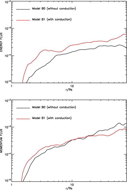
Upper panel: radial profile for energy fluxes (see equation 10) carried by wind for model B0 (black line) and B1 (red line). Lower panel: radial profile for momentum fluxes (see equation 11) carried by wind for model B0 (black line) and B1 (red line). From left to right, upper to bottom, the panels denote the density, temperature, radial velocity, and angular velocity, respectively.
Following previous analysis of wind, in Fig. 13, we plot the driving forces for wind in model B series. In both models, the main driving forces of wind are the combination of the gradient of magnetic pressure and gas pressure and the centrifugal force. The gas pressure gradient force is increased after conduction is considered consistent with the results in model A series. The centrifugal force in model B1 is two times of that in model B0. The increase of centrifugal force is because that in model B1, the rotational velocity of wind is larger than that in model B0 (see the lower-right panel of Fig. 11).
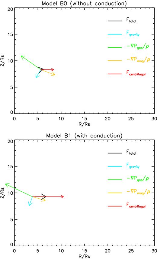
Force analysis at radius of 10Rs for model B0 (upper-panel, θ = 30°) and model B1 (lower-panel, θ = 20°).
4 SUMMARY AND DISCUSSION
Previous works have shown that strong winds exist in hot accretion flows (Yuan et al. 2015, see also Narayan et al. 2012; Yuan et al. 2012b; Li et al. 2013)1. Those works do not include thermal conduction. In extremely low accretion rate systems such as the accretion flow in Galactic centre Sgr A*, the plasma is very dilute, and the collisional mean-free path of electrons is large and much greater than their gyro-radius. Thus, thermal conduction is dynamically important and anisotropic, along magnetic field lines. In this paper, we have studied the effects of anisotropic thermal conduction on the wind by performing two-dimensional MHD simulations. Two different magnetic field topologies are considered: a strong-ordered field and a weaker tangled field. Our simulation results show that thermal conduction has moderate effects on the mass flux of wind in both cases. However, the energy flux of wind can be increased by a factor of 10 due to the increase in wind velocity when thermal conduction is included in ordered magnetic field case. The increase of wind velocity is because the driving forces (e.g. gas pressure gradient force and centrifugal force) increase when thermal conduction is included.
There are still some limitations in our work. Our simulations are two-dimensional and we adopt the one-temperature simplification. Ressler et al. (2015) study the two-temperature hot accretion flow with anisotropic conduction in GRMHD. Their results have shown that electron heating rates depend on the local magnetic field strength and electron thermal conduction modifies the electron temperature in the inner regions of accretion flows. They use a quadrupolar magnetic field and our model B1 is basically consistent with their results, such as the temperature gradient is flatter due to the effects of thermal conduction. But they did not give the results of wind properties.
Finally, we would like to mention that in a weakly collisional accretion flow, the ion mean-free path can be much greater than its gyro-radius, and thus the pressure tensor is anisotropic. In this case, the growth rate of the MRI can increase dramatically at small wave numbers compared with MRI in ideal MHD (Quataert, Dorland & Hammett 2002; Sharma, Hammett & Quataert 2003). In this regime, the viscous stress tensor is anisotropic, and Balbus (2004) has shown that when anisotropic viscosity is included, the flow is subject to the magnetoviscous instability (MVI; see also Islam & Balbus 2005). An interesting project in the future is to investigate the effects of MVI on wind from hot accretion flows.
We thank the referee for raising very useful questions, which help us to improve this paper significantly. We thank Feng Yuan and Fu-Guo Xie for the valuable discussions. DFB is supported in part by the National Basic Research Program of China (973 Program, grant 2014CB845800), the Strategic Priority Research Program The Emergence of Cosmological Structures of the Chinese Academy of Sciences (grant XDB09000000), and the Natural Science Foundation of China (grants 11103061, 11133005, 11121062, and 11573051). MCW is supported in part by the Natural Science Foundation of China (grants U1431228, 11133005, 11233003, 11421303), the National Basic Research Program of China (2012CB821801), the Strategic Priority Research Program of the Chinese Academy of Sciences (XDB09000000), and the grant from ‘the Fundamental Research Funds for the Central Universities’. This work made use of the High Performance Computing Resource in the Core Facility for Advanced Research Computing at Shanghai Astronomical Observatory.
REFERENCES
