


Abstract
In anticipation of the Gaia astrometric mission, a large sample of spectroscopic binaries has been observed since 2010 with the Spectrographe pour l'Observation des PHénomènes des Intérieurs Stellaires et des Exoplanètes spectrograph at the Haute–Provence Observatory. Our aim is to derive the orbital elements of double-lined spectroscopic binaries (SB2s) with an accuracy sufficient to finally obtain the masses of the components with relative errors as small as 1 per cent when the astrometric measurements of Gaia are taken into account. In this paper, we present the results from five years of observations of 10 SB2 systems with periods ranging from 37 to 881 d. Using the todmor algorithm, we computed radial velocities from the spectra, and then derived the orbital elements of these binary systems. The minimum masses of the components are then obtained with an accuracy better than 1.2 per cent for the 10 binaries. Combining the radial velocities with existing interferometric measurements, we derived the masses of the primary and secondary components of HIP 87895 with an accuracy of 0.98 and 1.2 per cent, respectively.
1 INTRODUCTION
Mass is the most crucial input in stellar internal structure modelling. It predominantly influences the luminosity of a star at a given stage of its evolution, and also its lifetime. The knowledge of the mass of stars in a non-interacting binary system, together with the assumption that the components have same age and initial chemical composition, allows the age and the initial helium content of the system to be determined and therefore to characterize the structure and evolutionary stage of the components. Such modelling provides insights into the physical processes governing the structure of the stars. Moreover, provided masses are known with great accuracy (Lebreton 2005), it gives constraints on the free physical parameters of the models. Therefore, modelling stars with extremely accurate masses (at the 1 per cent level), in different ranges of masses, would allow us to firmly anchor the models of the more loosely constrained single stars.
This paper is the third in a series dedicated to the derivation of accurate masses of the components of double-lined spectroscopic binaries (SB2) with the forthcoming astrometric measurements from the Gaia satellite. In paper I (Halbwachs et al. 2014), we have presented our programme to derive accurate masses from Gaia and from high-precision spectroscopic observations. We have selected a sample of 68 SB2s for which we expect to derive very precise inclination with Gaia, and M sin 3i with the Spectrographe pour l'Observation des PHénomènes des Intérieurs Stellaires et des Exoplanètes (SOPHIE spectrograph, Haute–Provence Observatory). Our objective is to determine for these SB2 systems the masses of the two components with an accuracy about 1 per cent. We have been observing these stars since 2010 with SOPHIE. The first result of our programme was the detection of the secondary component in the spectra of 20 binaries which were previously known as single-lined (paper I). Second result was the determination of masses for two SB2 with accuracy between 0.26 and 2.4 per cent, using astrometric measurements from Precision Integrated-Optics Nead-infrared Imaging ExpeRiment (PIONIER) and radial velocities (RVs) from SOPHIE (paper II).
Here, we present the accurate orbits measured for 10 SB2s (Table 1) with periods ranging from 37 to 881 d. After 5 yr of observations with SOPHIE, we collected a total of 123 spectra. In addition, a large number of previously published measurements is available for each of them in the SB9 catalogue (Pourbaix et al. 2004). Four of these targets are new SB2 identified in paper I, and previously known as SB1. Finally, we combined the RV measurements of one star (HIP 87895) with existing interferometric measurements and derive the masses of the two components.
10 SB2 analysed in this paper.
| HIP | HD | V | Perioda | |$N_{\rm spec}^{\phantom{spec}b}$| | Time spanc | SNRd |
| (mag) | (d) | (period) | ||||
| Previously published SB2 | ||||||
| 12081 | 15850 | 7.72 | 443.49 | 11 | 3.3 | 80 |
| 17732 | 23626 | 6.27 | 277.89 | 11 | 5.5 | 120 |
| 56275 | 100215 | 7.99 | 47.88 | 13 | 30.7 | 80 |
| 87895 | 163840 | 6.33 | 880.78 | 14 | 2.1 | 120 |
| 95575 | 183255 | 8.05 | 166.36 | 13 | 11.9 | 75 |
| 100321 | 195850 | 7.02 | 37.94 | 11 | 45.3 | 80 |
| SB2 identified in paper I, previously published as SB1 | ||||||
| 13791 | 18328 | 8.87 | 48.71 | 13 | 28.8 | 40 |
| 61727 | 110025 | 7.58 | 54.88 | 12 | 28.3 | 80 |
| 62935 | 120005 | 8.53 | 139.00 | 11 | 10.6 | 40 |
| 67195 | 120005 | 6.50 | 39.28 | 14 | 37.3 | 120 |
aThe period values are taken from the SB9 catalogue (Pourbaix et al. 2004).
bNspec gives the number of spectra collected with SOPHIE.
cThe time span is the total span of observation epochs, counted in number of periods.
dSNR is the median signal-to-noise ratio of each sample.
The observations are presented in Section 2. The method of measurements of RVs from SOPHIE's observations is explained in Section 3. We derive the orbital solutions in Section 4, discussing in particular the issue of the uncertainties when combining different data sets from different instruments. The derivation of the masses of HIP 87895 is discussed in Section 5. Finally, we summarize and conclude on our findings in Section 6.
2 OBSERVATIONS
The observations were performed at the T193 telescope of the Haute–Provence Observatory, with the SOPHIE spectrograph. SOPHIE is dedicated to the search of extrasolar planets, and, thanks to its high resolution (R ∼ 75 000), it enables accurate stellar RVs to be measured for SB2 components.
The spectra were all reduced through SOPHIE's pipeline, including localization of the orders on the frame, optimal order extraction, cosmic ray rejection, wavelength calibration, flat-fielding and bias subtraction. The minimum signal-to-noise ratio (SNR) is 40 for the faintest stars of the sample, but it may be as large as 150 for a 6 mag star. Before each observation run, ephemerides were derived from existing orbits provided by the SB9 catalogue (Pourbaix et al. 2004), and priority classes were assigned on the basis of the orbital phase. Four classes were used, the lowest priority corresponds to stars with expected RVs of primary and secondary component sufficiently different to permit accurate measurements, and the highest priority is reserved to the observations of the periastron of eccentric orbits.
Among all the observed SB2, we have selected those which were observed over at least one period, and which received a minimum of 11 observations. Table 1 summarizes this information. Given the very high quality of the measurements, an SB2 orbit could be derived in principle from only six of those observations, provided they were made at the most relevant phases. However, we show in Section 4 that 11 observations are necessary to validate the RV uncertainties, and to correct them when necessary.
3 RADIAL VELOCITY MEASUREMENTS
The RVs of the components are derived using the TwO-Dimensional CORrelation algorithm todcor (Zucker & Mazeh 1994; Zucker et al. 2004). It calculates the cross-correlation of an SB2 spectrum and two best-matching stellar atmosphere models, one for each component of the observed binary system. This two-dimensional cross-correlation function (2D-CCF) is maximized at the RVs of both components. The multi-order version of todcor, named todmor (Zucker et al. 2004), determines the RVs of both components from the gathering of 2D-CCF obtained from each order of the spectrum.
All SOPHIE multi-orders spectra were corrected for the blaze using the response function provided by SOPHIE's pipeline; then for each of them, the pseudo-continuum was detrended using a p-percentile filter (paper II, or e.g. Hodgson et al. 1985).
For both components of each binary, we determined the best-matching theoretical spectra from the phoenix stellar atmosphere models (Husser et al. 2013). We optimized the 2D-CCF with respect to effective temperature Teff, rotational broadening v sin i, metallicity [Fe/H], surface gravity log (g), and flux ratio at 4916 Å, α = F2/F1. Furthermore, each theoretical spectrum is convolved with the instrument line spread function, here modelled by a Gaussian, and pseudo-continuum detrended like the observed spectrum. The spectral parameters obtained through this method are given in Table 2. We determined spectral parameters from four spectra per binary on average, with the two components well individualized. The values and their uncertainties given in Table 2 are the average and standard deviation of the individual estimations. The 1σ uncertainties do not include known systematics of theoretical models with respect to real spectral types (see e.g. Torres et al. 2012).
The stellar parameters determined by optimization of the 2D-CCF obtained with todmor. Explanations in Section 3.
| HIP | Teff,1 | log g1 | V1sin i1a | [Fe/H] | α |
|---|---|---|---|---|---|
| HD | Teff,2 | log g2 | V2sin i2a | ||
| (K) | (dex) | (km s−1) | (dex) | (flux ratio) | |
| 12081 | 6290 | 4.24 | 11.9 | −0.37 | 0.635 |
| 15850 | ± 23 | ±0.05 | ±0.1 | ±0.01 | ±0.012 |
| 6003 | 4.30 | 6.5 | |||
| ± 13 | ±0.01 | ±0.1 | |||
| 13791 | 6173 | 4.31 | 5.5 | −0.34 | 0.034 |
| 18328 | ± 6 | ±0.01 | ±0.1 | ±0.01 | ±0.001 |
| 4953 | 5.09 | 0 | |||
| ± 95 | ±0.01 | ||||
| 17732 | 6030 | 3.34 | 9.4 | −0.71 | 0.258 |
| 23626 | ± 7 | ±0.03 | ±0.1 | ±0.01 | ±0.004 |
| 6051 | 3.84 | 0 | |||
| ± 18 | ±0.01 | ||||
| 56275 | 6889 | 3.93 | 20.6 | −0.33 | 0.036 |
| 100215 | ± 36 | ±0.11 | ±1 | ±0.01 | ±0.002 |
| 4906 | 4.33 | 0 | |||
| ± 75 | ±0.01 | ||||
| 61727 | 6461 | 3.82 | 9.8 | −0.48 | 0.070 |
| 110025 | ± 31 | ±0.15 | ±0.1 | ±0.06 | ±0.007 |
| 5256 | 4.31 | 7.7 | |||
| ± 168 | ±0.14 | 1.4 | |||
| 62935 | 5818 | 4.03 | 4.9 | −0.27 | 0.054 |
| 112138 | ± 85 | ±0.08 | ±0.4 | ±0.01 | ±0.015 |
| 4378 | 4.40 | 0 | |||
| ± 115 | ±0.13 | ||||
| 67195 | 6411 | 4.29 | 13.6 | −0.21 | 0.027 |
| 120005 | ± 29 | ±0.13 | ±0.2 | ±0.03 | ±0.002 |
| 4478 | 4.72 | 4.5 | |||
| ± 418 | ±0.21 | ±0.1 | |||
| 87895 | 5970 | 4.33 | 4.7 | −0.19 | 0.036 |
| 163840 | ± 1 | ±0.01 | ±0.1 | ±0.01 | ±0.004 |
| 4385 | 4.81 | 0 | |||
| ± 134 | ±0.04 | ||||
| 95575 | 4908 | 4.75 | 3.4 | −0.88 | 0.431 |
| 183255 | ± 5 | ±0.03 | ±0.1 | ±0.01 | ±0.008 |
| 4088 | 4.51 | 0 | |||
| ± 5 | ±0.03 | ||||
| 100321 | 6485 | 4.17 | 14.2 | −0.39 | 0.207 |
| 195850 | ± 6 | ±0.05 | ±0.2 | ±0.01 | ±0.011 |
| 5558 | 4.39 | 5.5 | |||
| ± 62 | ±0.04 | ± 1 |
aA null value is given to V sin i with no error bar whenever found less than SOPHIE's typical pixel size ∼2 km s−1.
It is worth mentioning that the derived metallicity [Fe/H] is systematically subsolar. Optimizing the CCF of several spectra of the Sun obtained by observing Vesta and Ceres with SOPHIE gave spectral parameters consistent with the known values for the Sun except metallicity that was found to be −0.33 dex. However, we kept the values of metallicity that maximized the 2D-CCF, as given in Table 2.
We then applied todmor to all multi-order spectra of each target and determined the RVs of both components discarding all orders harbouring strong telluric lines. For each of the non-discarded orders, we calculated a 2D-CCF, and used the maximum of this function to derive RVs for the primary and the secondary. Final velocities for each component are obtained by averaging these measurements and incorporating a correction for order-to-order systematics – typically 200–500 m s−1. The final velocities are displayed in Table 3. They are used to derive the orbital solutions for the 10 SB2 in the next section.
New radial velocities from SOPHIE and obtained with todmor. Outliers are marked with an asterisk (*) and are not taken into account in the analysis.
| BJD | RV1 | σRV1 | RV2 | σRV2 | O1−C1 | O2−C2 |
|---|---|---|---|---|---|---|
| −2400000 | (km s−1) | (km s−1) | (km s−1) | (km s−1) | (km s−1) | (km s−1) |
| HIP 12081 | ||||||
| 55440.6175 | −19.3006 | 0.0348 | 4.5327 | 0.0179 | 0.0498 | 0.0052 |
| 55532.3450 | 5.2930 | 0.0401 | −22.3033 | 0.0200 | −0.0023 | −0.0206 |
| 55605.3276 | −3.1655 | 0.0775 | −13.1499 | 0.0355 | −0.0492 | −0.0175 |
| 55784.5923 | −16.8235 | 0.0334 | 2.0058 | 0.0190 | 0.2120 | −0.0034 |
| 55864.4742 | −22.3574 | 0.0424 | 7.7735 | 0.0166 | −0.0294 | 0.0069 |
| 55933.2302 | 11.2363 | 0.0450 | −28.6746 | 0.0186 | 0.0576 | 0.0081 |
| 55966.2854 | 6.7183 | 0.0361 | −23.8320 | 0.0214 | 0.0144 | −0.0170 |
| 56148.6082 | −11.1919 | 0.1043 | −4.4740 | 0.0530 | −0.0939 | −0.0243 |
| 56243.3824 | −18.1414 | 0.0393 | 3.3409 | 0.0191 | 0.1222 | −0.0043 |
| 56323.3304 | −20.6003 | 0.0384 | 5.8376 | 0.0160 | −0.0433 | −0.0025 |
| 56889.6346 | 1.3632 | 0.0490 | −18.2750 | 0.0237 | −0.2906 | 0.0463 |
| HIP 13791 | ||||||
| 55605.3577 | −21.0198 | 0.0155 | 12.5004 | 0.2343 | −0.0602 | −0.3409 |
| 55784.6009 | −8.0152* | 0.0119* | 0.2619* | 0.2294* | −0.1650* | 9.5587* |
| 55864.4964 | −0.6383 | 0.0104 | −21.6297 | 0.1661 | 0.0092 | −0.1697 |
| 55965.3042 | 4.6405 | 0.0114 | −30.1618 | 0.1654 | 0.0038 | 0.2217 |
| 56148.6243 | −13.0655 | 0.0099 | −0.6196 | 0.1373 | 0.0105 | −0.1477 |
| 56243.4109 | −16.3507 | 0.0099 | 5.5330 | 0.1533 | 0.0154 | 0.4489 |
| 56323.3367 | −15.3310 | 0.0114 | 3.6038 | 0.1777 | −0.0089 | 0.2826 |
| 56525.5659 | −22.8333 | 0.0117 | 15.9524 | 0.1816 | 0.0041 | −0.0597 |
| 56526.6076 | −22.7883 | 0.0113 | 15.7956 | 0.1800 | 0.0231 | −0.1728 |
| 56618.4809 | −20.1445 | 0.0113 | 11.3540 | 0.1775 | −0.0036 | −0.1047 |
| 56701.3400 | 9.2144 | 0.0116 | −36.7152* | 0.2370* | 0.0088 | 1.3839* |
| 56890.6072 | 4.3730 | 0.0110 | −30.1670 | 0.1576 | −0.0229 | −0.1901 |
| 57009.3890 | −21.3907 | 0.0112 | 13.7637 | 0.1722 | 0.0158 | 0.1678 |
| HIP 17732 | ||||||
| 55532.4636 | −22.8766 | 0.0095 | 21.9980 | 0.0170 | 0.0019 | −0.0197 |
| 55784.6076 | −22.5330 | 0.0105 | 21.6484 | 0.0215 | 0.0016 | 0.0584 |
| 55933.2851 | 12.7972 | 0.0135 | −22.2329 | 0.0328 | 0.0123 | 0.0946 |
| 55965.3166 | 12.1605 | 0.0099 | −21.5826 | 0.0163 | 0.0003 | −0.0318 |
| 56243.4535 | 12.1444 | 0.0089 | −21.5210 | 0.0189 | 0.0060 | 0.0026 |
| 56323.3438 | −16.6398 | 0.0178 | 14.2097 | 0.0550 | 0.0020 | −0.0529 |
| 56525.5908 | 11.5734 | 0.0103 | −20.8293 | 0.0201 | −0.0154 | 0.0110 |
| 56618.4465 | −22.5381 | 0.0096 | 21.6251 | 0.0163 | −0.0060 | 0.0382 |
| 56890.6164 | −20.9656 | 0.0110 | 19.5609 | 0.0322 | 0.0023 | −0.0809 |
| 57009.3996 | 7.0245 | 0.0163 | −15.2479 | 0.0403 | −0.0123 | −0.0676 |
| 57073.3157 | 12.5569 | 0.0093 | −22.0421 | 0.0166 | 0.0009 | 0.0008 |
| HIP 56275 | ||||||
| 55692.3811 | 7.9257 | 0.0226 | −64.5112 | 0.1000 | 0.3626 | 0.0800 |
| 55863.6796 | −46.4777 | 0.0309 | 35.6378 | 0.1108 | 0.2361 | −0.0068 |
| 55933.6492 | 6.6220 | 0.0266 | −63.0758 | 0.0791 | 0.0026 | −0.2274 |
| 55966.5170 | −36.2910 | 0.0297 | 17.1534 | 0.1229 | 0.5121 | −0.1887 |
| 56243.6608 | −41.0739 | 0.0280 | 24.3508 | 0.1038 | −0.4721 | −0.0067 |
| 56323.5683 | −2.5587 | 0.0224 | −44.7952 | 0.1061 | 0.4674 | 0.2403 |
| 56413.3606 | 6.2006 | 0.0221 | −61.4924 | 0.0961 | 0.2601 | 0.1022 |
| 56414.3535 | 4.4350 | 0.0239 | −59.8103 | 0.0548 | −0.4309 | −0.2002 |
| 56700.5640 | 5.7582 | 0.0178 | −61.8093 | 0.1047 | −0.3363 | 0.0697 |
| 57009.6387 | −39.1607 | 0.0248 | 22.8202 | 0.0789 | 0.6746 | −0.1217 |
| 57073.4672 | −7.8378 | 0.0291 | −37.3543 | 0.1066 | −0.6925 | 0.0742 |
| 57159.4023 | −49.4717 | 0.0484 | 39.0880 | 0.1873 | −1.1735 | 0.5173 |
| 57160.3715 | −46.9715 | 0.0302 | 37.0594 | 0.0909 | 0.5892 | −0.1492 |
| HIP 61727 | ||||||
| 55605.5848 | −12.6740 | 0.0136 | 15.9258 | 0.1301 | −0.0215 | −0.3118 |
| 55693.3588 | 6.5327 | 0.0074 | −13.5889 | 0.0846 | −0.0088 | 0.3627 |
| 55933.6598 | −18.4952 | 0.0158 | 25.9363 | 0.2306 | −0.0041 | 0.5154 |
| 55965.6569 | 10.2366 | 0.0092 | −19.6786 | 0.1063 | 0.0244 | 0.0466 |
| 56034.4583 | −36.6083 | 0.0087 | 53.6952 | 0.1865 | −0.0076 | −0.2096 |
| 56323.6069 | 3.8442 | 0.0121 | −10.5547 | 0.1624 | 0.0030 | −0.8501 |
| 56413.4059 | −12.8533 | 0.0134 | 16.2369 | 0.1274 | −0.0334 | −0.2641 |
– continued
| BJD | RV1 | σRV1 | RV2 | σRV2 | O1−C1 | O2−C2 |
|---|---|---|---|---|---|---|
| −2400000 | (km s−1) | (km s−1) | (km s−1) | (km s−1) | (km s−1) | (km s−1) |
| 56700.6043 | −25.6469 | 0.0089 | 36.5198 | 0.1158 | 0.0088 | −0.1701 |
| 56764.3934 | 7.9839 | 0.0082 | −15.9285 | 0.1737 | 0.0235 | 0.2550 |
| 57009.6713 | 8.0070 | 0.0086 | −15.9493 | 0.1395 | 0.0020 | 0.3044 |
| 57073.5033 | −19.5056 | 0.0071 | 27.7723 | 0.2897 | 0.0283 | 0.7111 |
| 57159.4393 | 18.4660 | 0.0089 | −32.9927 | 0.2474 | −0.0225 | −0.2502 |
| HIP 62935 | ||||||
| 55605.6068 | −12.3906 | 0.0106 | 19.1954 | 0.1083 | −0.0079 | 0.5511 |
| 55933.7034 | 12.2587 | 0.0212 | −16.6646 | 0.2002 | −0.0453 | 1.0353 |
| 55965.6957 | 10.9649 | 0.0108 | −15.5176 | 0.1105 | −0.0205 | 0.2413 |
| 56034.4799 | −9.0670 | 0.0119 | 14.7234 | 0.1188 | 0.0067 | 0.9506 |
| 56323.6219 | −4.1875 | 0.0106 | 6.9054 | 0.1110 | −0.0224 | 0.3592 |
| 56413.4178 | −10.6338 | 0.0108 | 16.6760 | 0.1052 | 0.0037 | 0.6010 |
| 56414.3653 | −10.9714 | 0.0109 | 17.2867 | 0.1098 | −0.0001 | 0.7203 |
| 56619.6800 | 6.6032 | 0.0110 | −8.7968 | 0.1128 | 0.0060 | 0.5014 |
| 56700.6311 | −12.9241 | 0.0105 | 19.9558 | 0.1044 | 0.0065 | 0.5048 |
| 56763.4730 | 9.7161 | 0.0103 | −13.3344 | 0.1035 | 0.0370 | 0.5012 |
| 57073.5373 | 14.0341 | 0.0094 | −19.3651 | 0.0930 | 0.0212 | 0.8509 |
| HIP 67195 | ||||||
| 55693.4447 | −25.3810 | 0.0201 | 17.8880 | 0.1602 | −0.0487 | 0.0120 |
| 55965.7213 | −24.1047 | 0.0187 | 15.6821 | 0.1456 | −0.0092 | −0.0474 |
| 56033.4718 | −16.6905 | 0.0198 | 2.8186 | 0.1299 | −0.0100 | −0.0424 |
| 56323.6540 | −25.6179 | 0.0185 | 18.4821 | 0.1453 | 0.0131 | 0.0876 |
| 56323.7172 | −25.6252 | 0.0185 | 18.4805 | 0.1502 | 0.0034 | 0.0902 |
| 56324.4871 | −25.4322 | 0.0209 | 18.0313 | 0.1648 | 0.0304 | −0.0709 |
| 56324.5606 | −25.4128 | 0.0196 | 18.0605 | 0.1480 | 0.0177 | 0.0141 |
| 56413.4778 | 3.2056 | 0.0197 | −31.8507 | 0.1488 | 0.0263 | −0.2456 |
| 56414.4222 | 0.2645 | 0.0192 | −26.3836 | 0.1566 | 0.0138 | 0.1391 |
| 56526.3286 | 55.7540 | 0.0209 | −122.9667 | 0.1516 | −0.0025 | −0.1150 |
| 56763.4478 | 26.5703 | 0.0184 | −71.9675 | 0.1492 | 0.0100 | 0.2148 |
| 57073.5916 | −18.4045 | 0.0182 | 5.7351 | 0.1389 | −0.0178 | −0.0869 |
| 57159.4122 | 4.9344 | 0.0192 | −34.5608 | 0.1357 | 0.0026 | 0.0858 |
| 57160.4048 | 1.4943 | 0.0193 | −28.7538 | 0.1452 | −0.0216 | −0.0354 |
| HIP 87895 | ||||||
| 55306.5401 | −25.5851 | 0.0102 | −42.7398 | 0.1192 | −0.0824 | −0.2769 |
| 55440.3398 | −24.3803 | 0.0107 | −44.3309 | 0.1369 | 0.0012 | −0.1582 |
| 55692.5686 | −47.1465 | 0.0103 | −9.8598 | 0.1237 | −0.0269 | −0.3621 |
| 55783.4403 | −41.7373 | 0.0102 | −17.4182 | 0.1176 | −0.0231 | 0.3225 |
| 56034.6403 | −29.2514 | 0.0104 | −37.8613* | 0.1264* | −0.0441 | −1.0478* |
| 56148.4136 | −26.2422 | 0.0103 | −41.3782 | 0.1288 | 0.0258 | −0.0824 |
| 56243.2450 | −24.6700 | 0.0105 | −43.8842 | 0.1276 | 0.0358 | −0.2061 |
| 56324.6564 | −24.3659 | 0.0121 | −44.1758 | 0.1547 | 0.0306 | −0.0261 |
| 56413.6297 | −26.9424 | 0.0104 | −40.1199 | 0.1358 | 0.0005 | 0.1468 |
| 56414.5000 | −26.9901 | 0.0104 | −39.9479 | 0.1370 | 0.0080 | 0.2346 |
| 56414.5337 | −26.9911 | 0.0104 | −40.0227 | 0.1364 | 0.0091 | 0.1564 |
| 56525.3681 | −42.7839 | 0.0103 | −16.1425 | 0.1206 | −0.0066 | −0.0228 |
| 56763.6370 | −35.3359 | 0.0103 | −27.2716 | 0.1088 | 0.0394 | 0.1357 |
| 57159.5261 | −24.3802 | 0.0103 | −43.9809 | 0.1341 | 0.0306 | 0.1471 |
| HIP 95575 | ||||||
| 55306.6052 | −78.1722* | 0.0068* | −50.6807* | 0.0274* | −0.9557* | −0.9533* |
| 55440.3855 | −69.9864 | 0.0107 | −57.8756 | 0.0514 | −0.0113 | −0.0413 |
| 55693.5658 | −60.6375 | 0.0103 | −68.3909 | 0.0740 | −0.0148 | −0.0863 |
| 55784.4181 | −74.6558 | 0.0069 | −52.5504 | 0.0199 | 0.0121 | 0.0302 |
| 56034.5983 | −57.5141 | 0.0103 | −71.8023 | 0.0453 | 0.0156 | −0.0350 |
| 56147.4329 | −76.3749 | 0.0070 | −50.6872 | 0.0298 | 0.0013 | −0.0191 |
| 56243.2640 | −51.3445 | 0.0075 | −78.6904 | 0.0286 | −0.0033 | 0.0051 |
| 56414.5737 | −53.1692 | 0.0091 | −76.6845 | 0.0299 | −0.0014 | −0.0339 |
| 56619.2736 | −74.8908 | 0.0075 | −52.3081 | 0.0177 | 0.0033 | 0.0192 |
| 56890.4483 | −50.3115 | 0.0067 | −79.8551 | 0.0221 | −0.0060 | −0.0002 |
| 57073.6986 | −50.2649 | 0.0077 | −79.8382 | 0.0248 | 0.0093 | 0.0518 |
| 57159.5432 | −73.8810 | 0.0079 | −53.3993 | 0.0257 | 0.0044 | 0.0573 |
| 57295.3098 | −76.9201 | 0.0069 | −50.1277 | 0.0290 | −0.0122 | −0.0548 |
– continued
| BJD | RV1 | σRV1 | RV2 | σRV2 | O1−C1 | O2−C2 |
|---|---|---|---|---|---|---|
| −2400000 | (km s−1) | (km s−1) | (km s−1) | (km s−1) | (km s−1) | (km s−1) |
| HIP 100321 | ||||||
| 55440.4025 | 17.4467 | 0.0262 | −20.6978 | 0.0354 | −0.0453 | −0.0053 |
| 55693.6211 | −30.5121 | 0.0269 | 42.2770 | 0.0338 | −0.1057 | 0.0121 |
| 56147.4444 | −33.9387 | 0.0172 | 46.9496 | 0.0192 | 0.0303 | 0.0021 |
| 56243.2764 | 32.2481 | 0.0242 | −40.0539 | 0.0329 | 0.0321 | −0.0083 |
| 56414.6090 | −30.0393 | 0.0214 | 41.7375 | 0.0272 | −0.0196 | −0.0191 |
| 56525.4060 | −35.5108 | 0.0223 | 49.0625 | 0.0234 | 0.0698 | −0.0032 |
| 56526.4184 | −34.6986 | 0.0204 | 47.8903 | 0.0271 | −0.0222 | 0.0130 |
| 56619.4231 | 26.0449 | 0.0204 | −32.0577 | 0.0268 | −0.0975 | 0.0049 |
| 56890.5147 | 32.8145 | 0.0242 | −40.7347 | 0.0288 | 0.0780 | −0.0049 |
| 57159.5852 | 23.8836 | 0.0215 | −29.1134 | 0.0249 | −0.0255 | 0.0137 |
| 57160.5816 | 18.7741 | 0.0229 | −22.2593 | 0.0302 | 0.0997 | −0.0127 |
4 DERIVATION OF THE ORBITS
The orbital solutions for the 10 SB2 are derived by combining the new measurements presented in this paper with previously published RVs (references in Table 4).
| HIP | Reference of previous RV | Correction terms for previous measurements | Correction terms for new measurements | ||||||
|---|---|---|---|---|---|---|---|---|---|
| ε1,p | φ1,p | ε2,p | φ2,p | ε1,n | φ1,n | ε2,n | φ2,n | ||
| (km s−1) | (km s−1) | (km s−1) | (km s−1) | ||||||
| 12081 | Griffin (2005) | 0 | 0.615 | 0 | 0.565 | 0.1428 | 1 | 0.0061 | 1 |
| 13791 | Imbert (2006) | 0.24 | 1 | – | – | 0.0287 | 0.885 | 0.2689 | 0.885 |
| 17732 | Griffin & Suchkov (2003) | 0 | 0.272 | 0 | 0.759 | 0 | 1.101 | 0.0380 | 1.101 |
| 56275 | Griffin (2006) | 0 | 1.208 | 0 | 1.208 | 0.6909 | 0.905 | 0.2315 | 0.905 |
| 61727 | Halbwachs, Mayor & Udry (2012) | 0.3212 | 1 | – | – | 0.0261 | 0.911 | 0.4914 | 0.911 |
| 62935 | Griffin (2004) | 0 | 0.594 | – | – | 0.0294 | 1.101 | 0.1774 | 1.101 |
| 67195 | Shajn (1939) | 0 | 5.243 | – | – | 0.0175 | 1.046 | 0 | 0.8170 |
| 87895 | McAlister et al. (1995) | 0 | 0.342 | 0 | 0.342 | 0.0355 | 1.329 | 0.0662 | 1.329 |
| 95575 | Tokovinin (1991) | 1.022 | 1 | 1 | 1 | 0.0108 | 0.897 | 0.0399 | 0.897 |
| 100321 | Carquillat & Ginestet (2000) | 0 | 0.541 | 0 | 1.097 | 0.0665 | 1.017 | 0 | 0.572 |
Since several data sets coming from different instruments are used together to derive a common orbital solution, realistic errors should be attributed to each data set properly. It is explained in the following section. This process guarantees that each data set receives the proper weight with respect to all others, including the new SOPHIE measurements presented here.
4.1 Correction of uncertainties
Uncertainties of previously published measurements, when provided, are usually underestimated. On the other hand, many lists of RV measurements do not include uncertainties, but only weights (W). Therefore, two different procedures are applied to attribute correct uncertainties to these retrieved measurements. They are both based on the calculation of the F2 estimator of the goodness-of-fit (see paper II, equation 1, or Stuart & Ord 1994):
When the uncertainties are provided, a noise is quadratically added to the original uncertainties, in order to get exactly F2 = 0 for the SB1 orbit of each component. Since the original uncertainties are underestimated, this results in decreasing the variations of the relative weights of the measurements of a given component.
When only weights are given, they are first converted to uncertainties (|$\sigma =\sqrt{1/W}$|). Then they are scaled in order to get F2 = 0 for the SB1 orbit of each component.
Table 4 lists the derived values of the correction terms φ1, φ2, ε1 and ε2 for all stars of our sample.
The same procedure is applied to the uncertainties derived by todmor for the new measurements. For two binaries (HIP 67195 and HIP 100321), the SB1 orbit of the secondary component leads to a negative value of F2, implying that the uncertainties are slightly overestimated. In order to get F2 = 0, we preferred to keep the relative weights fixed, and simply multiply the uncertainties by a coefficient φ2 lower than 1.
All the RV measurements and the uncertainties used in the derivation of the orbits will be available through the SB9 catalogue (Pourbaix et al. 2004), which is accessible online.1
4.2 Derivation of the orbital elements
For each binary, we fitted an SB2 orbital model to the previously published data sets combined with the new SOPHIE observations. The parameters were optimized using a Levenberg–Marquard method.
The final orbital solution consists in the following orbital elements: the period, P, the eccentricity, e, the epoch of the periastron, T0, the longitude of the periastron for the primary component, ω1, the RV semi-amplitudes of each component, K1 and K2, and the RV of the barycentre, V0.
We also added three supplementary parameters, which are a systematic offset between the measurements previously published and the new ones, dn−p, and the offsets between the RVs of the primary and of the secondary component, |$d_{2-1}^p$| and |$d_{2-1}^n$|. The offset |$d_{2-1}^p$| is usually due to the fact that the published RVs were obtained from templates which are not specifically adapted to each component. For instance, a spectrovelocimeter like CORrelation – Radial – Velocities (Baranne, Mayor & Poncet 1979) was working by projecting any spectrum on a mask representing the spectrum of Arcturus. The offset between the primary and secondary RVs derived with todmor, |$d_{2-1}^n$| is expected to be null, but it is significant for some stars, since the spectra of the phoenix library do not perfectly represent the actual ones.
4.3 Results
Even with a correction, the uncertainties of the measurements from SOPHIE remain small and have weights much larger than the others. Therefore, incorporating the published data sets in the calculation essentially improved the accuracy of the period determined. Conversely, the significant precision of the new SOPHIE measurements allowed us to reach a very good accuracy on all other orbital parameters, especially the minimum masses.
The derived orbital elements for the 10 SB2 are given in Table 5. Among the 20 component stars, 15 of them have M sin 3i determined with an accuracy better than 0.7 per cent, while only 5 stars have minimum mass accuracies between 1 and 1.2 per cent.
The orbital elements derived from the previously published RV measurements and from the new ones. The radial velocity of the barycentre, V0, is in the reference system of the new measurements of the primary component. The minimum masses and minimum semimajor axes are derived from the true period (Ptrue = P × (1 − V0/c)).
| HIP | P | T0 (BJD) | e | V0 | ω1 | K1 | |${\cal M}_1 \sin ^3 i$| | a1sin i | N1 | dn − p | σ(O1 − C1)p, n |
|---|---|---|---|---|---|---|---|---|---|---|---|
| HD | K2 | |${\cal M}_2 \sin ^3 i$| | a2sin i | N2 | |$d^p_{2-1},d^n_{2-1}$| | σ(O2 − C2)p, n | |||||
| (d) | 2400000+ | (km s−1) | (o) | (km s−1) | (|${\cal M}_{\odot }$|) | (Gm) | (km s−1) | (km s−1) | |||
| 12081 | 443.288 | 55905.74 | 0.584 94 | −7.883 | 283.66 | 16.784 | 0.5493 | 82.98 | 47+11 | −1.141 | 0.634, 0.128 |
| 15850 | ±0.023 | ±0.12 | ±0.000 54 | ±0.046 | ±0.10 | ±0.057 | ±0.0019 | ±0.28 | ±0.101 | ||
| 18.258 | 0.5050 | 90.261 | 47+11 | −0.208, −0.064 | 0.548, 0.020 | ||||||
| ±0.015 | ±0.0034 | ±0.052 | ±0.124, ±0.050 | ||||||||
| 13791 | 48.708 95 | 55050.392 | 0.187 81 | −8.537 | 55.26 | 16.030 | 0.2405 | 10.5456 | 33+12 | 0.686 | 0.431, 0.022 |
| 18328 | ±0.000 23 | ±0.043 | ±0.000 78 | ±0.012 | ±0.29 | ±0.015 | ±0.0027 | ±0.0090 | ±0.078 | ||
| 27.07 | 0.142 41 | 17.809 | 0+11 | ⋅⋅⋅, 0.400 | ⋅⋅⋅, 0.246 | ||||||
| ±0.14 | ±0.000 94 | ±0.089 | ⋅⋅⋅, ±0.096 | ||||||||
| 17732 | 277.9500 | 55230.207 | 0.143 19 | −2.918 | 159.14 | 18.6644 | 1.1359 | 70.598 | 41+11 | −1.096 | 0.505, 0.0080 |
| 23626 | ±0.0074 | ±0.095 | ±0.000 83 | ±0.011 | ±0.14 | ±0.0051 | ±0.0019 | ±0.022 | ±0.058 | ||
| 23.208 | 0.9135 | 87.784 | 41+11 | 0.279, 0.116 | 1.670, 0.054 | ||||||
| ±0.017 | ±0.0010 | ±0.067 | ±0.169, ±0.027 | ||||||||
| 56275 | 47.894 10 | 56781.809 | 0.2317 | −17.879 | 247.52 | 28.00 | 1.5007 | 17.94 | 31a+13 | −1.273 | 1.299, 0.571 |
| 100215 | ±0.000 89 | ±0.080 | ±0.0018 | ±0.18 | ±0.71 | ±0.18 | ±0.0086 | ±0.11 | ±0.294 | ||
| 51.709 | 0.8126 | 33.128 | 10+13 | 0.963, 0.273 | 3.786, 0.207 | ||||||
| ±0.087 | ±0.0090 | ±0.051 | ±1.247, ±0.202 | ||||||||
| 61727 | 54.878 64 | 56476.6509 | 0.347 44 | −1.5628 | 185.679 | 30.842 | 1.432 | 21.823 | 43+12 | 0.168 | 0.639, 0.020 |
| 110025 | ±0.000 18 | ±0.0072 | ±0.000 51 | ±0.0093 | ±0.057 | ±0.019 | ±0.017 | ±0.011 | ±0.097 | ||
| 48.51 | 0.9104 | 34.33 | 0+12 | ⋅⋅⋅, 0.358 | ⋅⋅⋅, 0.435 | ||||||
| ±0.26 | ±0.0060 | ±0.18 | ⋅⋅⋅, ±0.142 | ||||||||
| 62935 | 139.0081 | 55680.66 | 0.1508 | 0.244 | 31.37 | 15.643 | 0.4791 | 29.557 | 89+11 | −0.189 | 0.680, 0.022 |
| 112138 | ±0.0027 | ±0.17 | ±0.0018 | ±0.011 | ±0.44 | ±0.023 | ±0.0049 | ±0.038 | ±0.065 | ||
| 23.03 | 0.3254 | 43.51 | 0+11 | ⋅⋅⋅, 0.416 | ⋅⋅⋅, 0.245 | ||||||
| ±0.11 | ±0.0020 | ±0.20 | ⋅⋅⋅, ±0.071 | ||||||||
| 67195 | 39.284 974 | 56211.2841 | 0.785 84 | −9.532 | 325.250 | 45.44 | 1.1731 | 15.181 | 37+14 | −1.113 | 5.027, 0.021 |
| 120005 | ±0.000 091 | ±0.0045 | ±0.000 50 | ±0.016 | ±0.031 | ±0.12 | ±0.0062 | ±0.026 | ±0.864 | ||
| 78.86 | 0.6760 | 26.346 | 0+14 | ⋅⋅⋅, −0.013 | ⋅⋅⋅, 0.118 | ||||||
| ±0.22 | ±0.0034 | ±0.048 | ⋅⋅⋅, ±0.050 | ||||||||
| 87895 | 881.629 | 55650.40 | 0.4165 | −32.346 | 135.47 | 11.393 | 0.9869 | 125.57 | 106+14 | 0.456 | 0.842, 0.035 |
| 163840 | ±0.065 | ±0.49 | ±0.0014 | ±0.015 | ±0.26 | ±0.021 | ±0.0097 | ±0.22 | ±0.047 | ||
| 17.374 | 0.6471 | 191.50 | 16+13 | −0.754, 0.319 | 1.210, 0.210 | ||||||
| ±0.077 | ±0.0041 | ±0.84 | ±0.608, ±0.058 | ||||||||
| 95575 | 166.8351 | 56087.993 | 0.13698 | −64.2928 | 63.21 | 14.0202 | 0.23291 | 31.866 | 23+12 | 0.394 | 1.225, 0.0098 |
| 183255 | ±0.0031 | ±0.094 | ±0.00031 | ±0.0040 | ±0.20 | ±0.0048 | ±0.00051 | ±0.011 | ±0.233 | ||
| 15.696 | 0.20804 | 35.675 | 9+12 | 0.356, 0.097 | 1.981, 0.044 | ||||||
| ±0.016 | ±0.00028 | ±0.037 | ±0.592, ±0.014 | ||||||||
| 100321 | 37.939920 | 56254.291 | 0.18242 | 0.941 | 111.043 | 34.306 | 1.06199 | 17.596 | 52+11 | 0.324 | 0.530, 0.068 |
| 195850 | ±0.000081 | ±0.010 | ±0.00025 | ±0.023 | ±0.096 | ±0.025 | ±0.00081 | ±0.013 | ±0.079 | ||
| 45.0916 | 0.8080 | 23.1284 | 49+11 | 0.493, 0.121 | 1.160, 0.011 | ||||||
| ±0.0089 | ±0.0011 | ±0.0041 | ±0.174, ± 0.028 |
aThe three first measurements in Griffin (2006) were discarded.
A comparison between the standard deviation of the residuals of the previous measurements and of the new ones also illustrates the improvements due to SOPHIE. It results from the last column of Table 5 that σ(O−C)p is between 2.3 and 239 times larger than σ(O−C)p, with a median around 30.
The orbital solutions, including previously published measurements, are displayed in Fig. 1. The (O−C) residuals are included in Table 3 and are plotted in Fig. 2. We do not observe any drift for any of the 10 SB2.
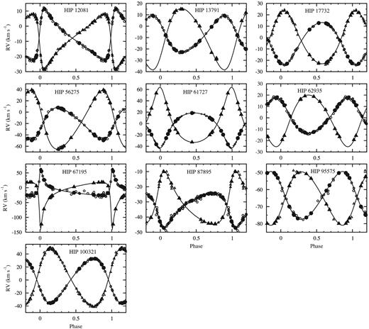
The spectroscopic orbits of the 10 SB2; the circles refer to the primary component, and the triangle to the secondary; the large filled symbols refer to the new RV measurements obtained with SOPHIE. For each SB2, the RVs are shifted to the zero-point of the SOPHIE measurements of the primary component.
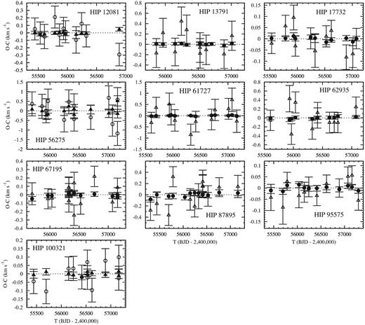
The residuals of the RVs obtained from todmor for the 10 SB2s. The circles refer to the primary component and the triangles to the secondary component. For readability, the residuals of the most accurate RV measurements are in filled symbols.
5 COMBINED ORBITAL SOLUTION AND MASSES FOR HIP 87895
HIP 87895 is the close visual binary (VB) MCA 50. Among the many observations recorded in the online Fourth Catalogue of Interferometric Measurements of Binary Stars,2 (Third Catalog; Hartkopf, McAlister & Mason 2001) we found three very accurate long-base interferometric measurements performed with the Palomar Testbed Interferometer (PTI). Since the RV measurements are already providing parameters common to the spectroscopic and to the visual orbits, three two-dimensional measurements are quite sufficient to derive the remaining ones, which are the orbital inclination, i, the position angle of the nodal line, Ω, and the apparent semimajor axis or the trigonometric parallax (both may equally be used).
These measurements and the rescaled error ellipsoids provided by Muterspaugh et al. (2010) are taken into account simultaneously with our RV measurements, in order to directly derive the masses of the components and the trigonometric parallax of the system.
The results are given in Table 6 and in Fig. 3. We derived the two masses with accuracies of 1.2 and 0.98 per cent, respectively.
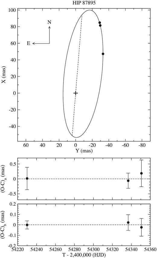
The visual part of the combined orbit of HIP 87895.Upper panel: the visual orbit; the circles are the three positions obtained from long-base interferometry; the node line is in dashes. Middle panel: the residuals along the semimajor axis of the error ellipsoid. Lower panel: the residuals along the semiminor axis of the error ellipsoid.
The combined VB+SB2 solutions of HIP 87895. For consistency with the SB orbits and with the forthcoming astrometric orbit, ω refer to the motion of the primary component.
| HIP 87895 | |
|---|---|
| P (d) | 881.628 ± 0.064 |
| T0 (BJD-2400000) | 55650.39 ± 0.38 |
| e | 0.4165 ± 0.0010 |
| V0 (km s−1) | −32.347 ± 0.014 |
| ω1 (o) | 135.46 ± 0.16 |
| Ω(o; eq. 2000) | 175.32 ± 0.44 |
| i (o) | 72..83 ± 0.47 |
| ex a (mas) | 80.64 |
| |${\cal M}_1$| (|${\cal M}_{\odot }$|) | 1.132 ± 0.014 |
| |${\cal M}_2$| (|${\cal M}_{\odot }$|) | 0.7421 ± 0.0073 |
| ϖ (mas) | 36.35 ± 0.20 |
| dn−p (km s−1) | 0.456 ± 0.047 |
| d2−1 p (km s−1) | −0.754 ± 0.608 |
| d2−1 n (km s−1) | 0.320 ± 0.056 |
| σ(O–C) PTI (mas) | 0.086 |
| σ(O–C) RV p (km s−1) | 0.841, 1.211 |
| σ(O–C) RV n (km s−1) | 0.035, 0.209 |
6 SUMMARY AND CONCLUSION
We obtained for 10 SB2 new RV measurements from spectra taken with SOPHIE, among which 4 new SB2 are identified in paper I. The todmor algorithm was used to separate the two components in each spectrum. All 10 systems had previously published measurements in archive, which we added to our measurements to calculate the orbital solutions. We also derived estimations of stellar parameters obtained by optimizing the two-dimensional cross-correlation obtained with todmor.
We achieved the objective of deriving minimum mass with an accuracy better than 1 per cent for 15 of the 20 stars of our SB2 sample. Moreover, all 10 binaries have the minimum mass of both components estimated with relative uncertainties lower than 1.2 per cent. This is a great achievement of the combination of todmor and SOPHIE. Especially it did very well in extreme configurations such as with small SNR (∼40), and very small flux ratio (α < 0.05) between the two components.
We combined our RV measurements of HIP 87895 with three relative positions derived from long-based interferometric observations, and we obtained new mass estimate of the components, M1 = 1.132 ± 0.014 M⊙ and M2 = 0.7421 ± 0.0073 M⊙. On the basis of speckle observations, McAlister et al. (1995) previously derived M1 = 1.16 ± 0.12 M⊙ and M2 = 0.77 ± 0.05 M⊙, i.e. with relative errors of 10 and 6 per cent. Therefore, our measurements refine profitably to the 1 per cent level the confidence range on the masses of HIP 87895.
Added to the systems observed with pionier, we have now three binaries observed with SOPHIE which may be used to check the masses that will be derived from Gaia.
The project is based on observations performed at the Observatoire de Haute–Provence (CNRS), France and was supported by the French INSU-CNRS ‘Programme National de Physique Stellaire’ and ‘Action Spécifique Gaia’. We are grateful to the staff of the Haute–Provence Observatory, and especially to Dr F. Bouchy, Dr H. Le Coroller, Dr M. Véron, and the night assistants, for their kind assistance. We made use of the SIMBAD data base, operated at CDS, Strasbourg, France. This research has received funding from the European Community's Seventh Framework Programme (FP7/2007-2013) under grant-agreement numbers 291352 (ERC). The authors are very thankful to the anonymous reviewer for his help to improve the quality of this paper.
REFERENCES
